| Issue |
A&A
Volume 700, August 2025
|
|
|---|---|---|
| Article Number | A29 | |
| Number of page(s) | 16 | |
| Section | Stellar structure and evolution | |
| DOI | https://doi.org/10.1051/0004-6361/202553935 | |
| Published online | 29 July 2025 | |
A Hα metric for identifying dormant black holes in X-ray transients
1
Instituto de Astrofísica de Canarias, E-38205 La Laguna, Tenerife, Spain
2
Departamento de Astrofísica, Universidad de La Laguna, E-38206 La Laguna, Tenerife, Spain
⋆ Corresponding author: This email address is being protected from spambots. You need JavaScript enabled to view it.
Received:
28
January
2025
Accepted:
3
June
2025
Abstract
Dormant black holes in X-ray transients can be identified by the presence of broad Hα emission lines from quiescent accretion discs. Unfortunately, short-period cataclysmic variables can also produce broad Hα lines, especially when viewed at high inclinations, and are thus a major source of contamination. Here we compare the full width at half maximum (FWHM) and equivalent width (EW) of the Hα line in a sample of 20 quiescent black hole transients and 354 cataclysmic variables (305 from SDSS I to IV) with secure orbital periods (Porb) and find that: (1) FWHM and EW values decrease with Porb, and (2) for a given Porb both parameters are typically larger in black hole transients than in cataclysmic variables. We also compile spectral types for 17 low-mass companions in black hole transients from the literature and derive an empirical Porb − Teff calibration. Using this, we conclude that the decrease in EW with Porb is mostly driven by the dilution of the Hα flux by the donor star continuum, which dominates the r-band spectrum for Porb ≳ 0.2 d. At shorter periods, the larger contribution of the disc to the total r-band flux introduces significant scatter in the EWs due to the changing visibility of the disc projected area with binary inclination. On the other hand, the larger EWs observed in black holes can be explained by their extreme mass ratios (which limit the fractional contribution of the companion to the total flux) and the absence of a white dwarf component (important at Porb ≲ 0.085 d). Finally, we present a tentative metric, based on Hα FWHM and EW information, and provide optimal cuts to select ∼80% of the black hole X-ray transients, while rejecting ∼78% of the cataclysmic variables in our sample. Such a metric, combined with other multi-frequency diagnostics, can help detect new dormant black hole X-ray transients in blind large-scale surveys such as HαWKs and its pathfinder, Mini-HαWKs.
Key words: accretion, accretion disks / black hole physics / line: profiles / stars: dwarf novae / novae, cataclysmic variables
© The Authors 2025
 Open Access article, published by EDP Sciences, under the terms of the Creative Commons Attribution License (https://creativecommons.org/licenses/by/4.0), which permits unrestricted use, distribution, and reproduction in any medium, provided the original work is properly cited.
This article is published in open access under the Subscribe to Open model. This email address is being protected from spambots. You need JavaScript enabled to view it. to support open access publication.
1. Introduction
Over the past 50 years, black hole X-ray transients (BH XRTs) have provided us with special windows through which to study accretion processes in extreme environments, supernova explosions, and the evolution of close binary systems. In recent years, other BH populations have also been revealed by gravitational wave detectors (Abbott et al. 2019) and Gaia astrometry (e.g. Panuzzo 2024). In this context, XRTs remain a key benchmark for BH properties, as they are supposed to descend from a well-defined binary evolution channel at near solar metallicity, involving a common envelope phase (but see Naoz et al. 2016, also Burdge et al. 2024, for an alternative formation pathway in hierarchical triples).
With only 20 dynamically confirmed cases and another ≈50 candidates (Corral-Santana et al. 2016), the current sample of BH XRTs is severely limited by small numbers. In addition, the sample is X-ray selected, and thus biased towards transients with short recurrence times and high outburst luminosities (Wu et al. 2010; Lin & Yan 2019). Other complex X-ray selection biases may also be at play, such as high-inclination BHs concealed by disc obscuration (Narayan & McClintock 2005; Corral-Santana et al. 2013), a potential lack of short-period (< 4 h), radiatively inefficient BH transients (Knevitt et al. 2014, see also Arur & Maccarone 2018), period gap BH XRTs with very low X-ray luminosities (Maccarone & Patruno 2013), or the possible existence of faint, persistent (i.e. non-transient) BH X-ray binaries with long orbital periods (Menou et al. 1999). In addition, both the Galactic distribution of XRTs and their BH masses are likely to be shaped by natal kicks (Gandhi et al. 2020) and obscuration by interstellar extinction (Jonker et al. 2021). Similarly, while the existence of the so-called lower mass-gap (i.e. dearth of BHs with masses between ≃2 − 5 M⊙), appears robust against transient selection effects (Siegel et al. 2023), it depends critically on our ability to measure accurate masses in the presence of accretion disc contamination (Kreidberg et al. 2012). A significant step forward in the statistics of BH XRTs, with a more cleanly selected sample, is therefore fundamental to disentangling selection biases and advancing our knowledge of this reference population.
In an attempt to increase the number of BH XRTs, we have developed a series of scaling relations between fundamental binary parameters and the properties of the Hα emission line, formed in the accretion disc around the BH (Casares 2015, 2016; Casares et al. 2022). In particular, a correlation between the Hα full width at half maximum (FWHM) and the radial velocity semi-amplitude of the companion star (K2) allows for the extraction of compact object mass functions in systems where the spectrum of the donor star is not detected (Casares 2015; hereafter C15). This requires independent knowledge of the orbital period, which can be obtained from light curve variability. If the FWHM is also measured photometrically, this opens up the new concept of ‘photometric mass function’, whereby BHs can be searched for and weighed photometrically in large fields of view, i.e. much more efficiently than by classical spectroscopy (see C15).
In Casares (2018) (hereafter C18), we present a proof ofconcept of how to obtain Hα FWHMs using three custom interference filters of different widths. We also propose a new strategy (HαWKs, an acronym for ‘Hα-Width Kilodegree survey’)optimised for the detection of dormant1 BH XRTs in a blind survey of the Galactic plane. In addition to Hα widths, the HαWKs photometric system also provides equivalent width (EW) information. Furthermore, as the three filters are centred at 6563 Å, the results are invariant to interstellar extinction and the spectral energy distribution of the objects. HαWKs was subsequently validated in a feasibility test, demonstrating that Hα FWHM and EW values can be recovered within 10% accuracy in a sample of quiescent BH XRTs down to at least r = 22 (Casares & Torres 2018). Essentially, HαWKs exploits the width of the Doppler-broadened Hα line as a proxy for the deep gravitational fields of compact stars, enabling the efficient selection of dormant BHs. To some extent, the approach is similar to reverberation mapping techniques, whereby line widths from the broad line region are used to weigh super-massive BHs in active galactic nuclei (e.g. Peterson et al. 2004).
A search for dormant BHs with HαWKs would in principle be free from X-ray selection bias, although the strategy does favour the detection of accreting binaries with short periods and high inclinations (i.e. large Hα widths). The main source of contamination at large FWHMs is expected to come from cataclysmic variables (CVs i.e. interacting binaries with accreting white dwarfs), which are extremely abundant compared to BH XRTs. Monte Carlo simulations have shown that a cut-off at FWHM ≳ 2200 km s−1 removes ≈99.9% of all the CVs, while retaining ≈50% of the BHs (C18). The recovery of BHs with FWHM < 2200 km s−1 is quite challenging as the level of CV contamination increases dramatically. The aim of this paper is to develop a metric based on Hα FWHMs and EW information from a large sample of quiescent BH XRTs and CVs, to help separate these two populations. The new diagnostic will provide an additional tool to identify dormant BH XRTs in single epoch spectra and special photometric Hα surveys such as HαWKs and its pathfinder, Mini-HαWKs.
2. Updated collection of Hα FWHM and EWs in quiescent BH XRTs
Table 1 gives a list of FWHM and EW measurements of the Hα line in 20 quiescent BH XRTs. These were obtained from a spectroscopic database collected over several epochs spanning 30 years. The errors reported include systematic uncertainties to account for orbital and secular (inter-epoch) variability. Appendix A gives full details of the database (broken down into different epochs), how FWHM and EW values were measured, and the systematic uncertainties applied. The numbers for XTE J1650-500 should be treated with caution, as the only available spectra were taken just ≈9 months after the peak of the outburst, when the binary was still fading into quiescence (see Sánchez-Fernández et al. 2002, also Appendix A for a photometric verification). Similarly, the GX 339-4 off-state data from Heida et al. (2017) used here might not correspond to complete quiescence due to the frequent outburst activity characteristic of this system. It should be emphasised that the quiescent FWHM and EW values for each system are quite stable over time, despite orbital and secular variability (Appendix A).
FWHM and EW of Hα lines in quiescent BH XRTs.
2.1. FWHM versus orbital period
Figure 1 displays the behaviour of the FWHM as a function of the orbital period (Porb) for the ensemble of BH XRTs. For comparison, we also plot FWHM values of 43 quiescent CVs (mostly dwarf novae) from C15, using red triangles. This sample was selected from Ritter & Kolb’s catalogue (Ritter & Kolb 2003) based on accurate reports of the radial velocity curve of the companion star and is therefore prone to selection biases. In particular, it over-represents CVs with long Porb, where the companion’s spectrum dominates, and eclipsing short Porb CVs, where K2 is inferred through light curve modelling. To compensate for the uneven Porb distribution we have added 305 CVs from the Sloan Digital Sky Survey (SDSS) I to IV with secure Porb determinations (Inight et al. 2023). The latter is a magnitude-limited spectroscopic sample and is therefore more uniformly selected. The SDSS CVs have been divided into three classes: magnetic (intermediate polars, polars, and pre-polars), nova-likes, and dwarf novae (including WZ Sge, SU UMa, U Gem, and Z Cam sub-types). Eclipsing CVs are indicated by open triangles, although the list is likely to be incomplete as some SDSS CVs lack sufficient photometric coverage for eclipse detection. Typical FWHM uncertainties for SDSS CVs are smaller than the symbol size because they are obtained from individual (single epoch) spectra. More realistic uncertainties (including orbital and secular variability) have been estimated at the ≈7% level in C15.
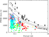 |
Fig. 1. Distribution of BH XRTs (black circles) and CVs (triangles) in the FWHM-Porb plane. Open triangles indicate eclipsing CVs, while filled triangles non-eclipsing CVs. Red triangles represent 43 CVs from C15 and blue or cyan, green, and yellow triangles the 305 SDSS CVs of dwarf novae, magnetic, and nova-like types, respectively (Inight et al. 2023). For reference, we indicate the maximum FWHM for a Chandrasekhar-mass white dwarf viewed edge-on, and the lower limit of the FWHM for accretion disc eclipses of a typical 0.82 M⊙ CV white dwarf (dotted line). We also plot the maximum FWHM of a 2.3 M⊙ neutron star viewed edge-on. The expected track of a canonical 7.8 M⊙ BH seen at 60° inclination is represented by the dashed line. |
Figure 1 is an update of Fig. 9 from C18, with the addition of six more BH XRTs and the 305 SDSS CVs. Since FWHM scales with K2 (C15), the mass function equation  can be used to draw Porb − FWHM lines for a given set of compact object mass (M1), mass ratio (q), and binary inclination (i). As a guide, we have marked an approximate upper bound for FWHM in CVs, based on the Chandrasekhar mass limit and a maximum binary inclination of i = 90°. Here, we have also adopted the Porb − q relation q = 0.73 − 11.55 × exp[−(Porb+0.39)/0.15], derived in C18, and the q dependence of the FWHM − K2 correlation (Equations (5) and (6) in C15). In addition, following C18 we have drawn a lower limit on FWHM for accretion disc eclipses of a representative 0.82 M⊙ white dwarf (Zorotovic et al. 2011). An upper limit on FWHM for the case of an extreme neutron star mass, M1 = 2.3 M⊙ (Ruiz et al. 2018; Shibata et al. 2019) at i = 90°, is also indicated.
Figure 1 shows that, for a given Porb, BH XRTs naturally produce broader Hα lines than CVs due to the more massive central objects. As a matter of fact, BH XRTs closely follow the predicted FWHM − Porb curve for a canonical BH mass of M1 = 7.8 M⊙ (Özel et al. 2010; Kreidberg et al. 2012) with a typical q = 0.06 (Casares 2016) and most probable inclination of i = 60° (dashed line). Only GRO J0422+32 and GX339-4 fall under the 2.3 M⊙ neutron star limit, placing them in the CV region. In the case of GRO J0422+32, this is consistent with a low-mass BH (2.7 M⊙) viewed at an inclination of i = 56° (see Casares et al. 2022). For GX 339-4, the low FWHM value could be due to either a light BH or a low inclination (Heida et al. 2017). Since Fig. 1 is a representation of the mass function itself, it provides an efficient way to identify BHs. As is discussed in C18, BHs are easily selected above FWHM ≳ 2200 km s−1 since CV intruders over this limit must have a short Porb ≲ 2.1 h (i.e. below the period gap) and are likely to be eclipsing. On the other hand, additional information (such as Porb) is needed to clearly separate BHs from CVs belowFWHM ≲ 2200 km s−1.
2.2. EW versus orbital period
In Fig. 2 we plot the behaviour of EWs versus Porb for the same sample of BH XRTs and CVs as in Fig. 1. Again, the error bars for the EWs of the SDSS CVs are not shown as they are smaller than the symbol size. Realistic errors, including orbital and secular variability, are estimated at the ≈14% level (see C15). Similar to the FWHM case, we observe that (i) EWs tend to increase with decreasing Porb, and (ii) BH EWs are typically larger than CV EWs at the same Porb. This is illustrated by the blue histogram, which represents the mean EW for CVs calculated in ten uniform bins of size Δlog Porb = 0.2. Only XTE J1650-500 has an EW significantly below the CV mean for its Porb, but as was mentioned earlier this is due to the fact that the spectra were obtained when the system had not yet reached true quiescence2.
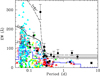 |
Fig. 2. EW versus Porb for the same sample of BHs and CVs as in Fig. 1. For reference we plot BH EW lines of constant inclination (i = 33°, 60° and 80°), computed with our toy model simulation (see Appendix C for details). The blue histogram indicates the mean EW for CVs in ten period bins. |
To understand the EW evolution with Porb, we have built a toy model that generates synthetic EWs based on the Roche geometry and the continuum blackbody radiation associated with the donor star and the accretion disc. The Hα emission is set to arise from the surface of the disc and it is assumed to be optically thin. A key ingredient of the model is the Porb dependence of the donor effective temperature, which we have calibrated in Appendix B using Eq. (B.2). The latter was derived from a compilation of empirical spectral types of BH donors (Table B.1) and CV donors from Knigge (2006). In the case of BH binaries we fixed q = 0.06 (Casares 2016, also Table B.3), while for CVs we adopted the aforementioned exponential increase with Porb, i.e. q = 0.73 − 11.55 × exp[−(Porb+0.39)/0.15]. In the case of CVs, we also added an extra blackbody to account for the emission from the white dwarf. Further details of the modelling are given in Appendix C.
The black lines shown in Fig. 2 represent the BH EWs predicted by our model for three different inclinations: 33°, 60°, and 80°, i.e. the median and extremes containing 68% of the values for an isotropic distribution of orientations. We observe that, despite the very rough approximations involved, our model is able to provide a qualitative description of the behaviour of the BH EWs with Porb. Overall, the increase in BH EWs with decreasing Porb is explained by the reduction in donor stellar flux caused by the drop in temperature, which becomes more pronounced at Porb < 0.3 d (see Fig. B.1). As a consequence, the accretion disc becomes the dominant source of continuum light at Porb ≲ 0.2 d and, due to the foreshortening caused by binary inclination, a wider range of EW values is expected at these short orbital periods.
As is shown in Appendix C, the model is also able to reproduce the larger EWs observed in BHs simply by invoking their smaller q values (see Fig. C.2). This has the effect of reducing the relative contribution of the donor star to the continuum flux, increasing the EW of the Hα line. Only at very short periods below the period gap (Porb ≲ 0.085 d) do CV mass ratios become comparable to the ones of BHs, but then the white dwarf contribution starts to dominate over the donor’s continuum in the Hα region, keeping the EW values of CVs below the EWs of BHs. Obviously the model is far too simplistic to explain the scatter seen in systems with similar Porb, mass ratios and inclinations. Different accretion disc structures and the intrinsicvariability in the continuum and/or the Hα flux (perhaps in response to irradiation, e.g. Hynes et al. 2002, 2004) are also likely to play an important role in the observed EW values.
We have so far avoided quiescent XRTs with neutron stars in this paper. This is because the number of systems with available quiescent FWHM and EW measurements is limited to Cen X-4 and XTE J2123-058 (see Table 3 in C15). A third obvious candidate, Aql X-1, is unfortunately contaminated by a very bright interloper (Chevalier et al. 1999; Mata Sánchez et al. 2017), which biases the EW and FWHM determination. Cen X-4 and XTE J2123-058 fall in regions of the Porb-FWHM and Porb-EW diagrams populated by CVs, and therefore cannot be unambiguously identified. This is not surprising given the comparable mass ratios and compact object masses of the two populations.
3. A Hα metric for selecting quiescent BH XRTs
In this section we exploit the orbital period dependence of the FWHM and the EW of Hα lines in BH XRTs to facilitate the selection of new dormant BHs. A least-squares power-law fit to the BH FWHM data versus Porb yields FWHM  , with FWHM expressed in units of kilometers per second and Porb in days. The choice of a power law is physically motivated by the mass function equation, i.e. FWHM
  . We have not considered the error bars in the fit to avoid this being dominated by points with a low FWHM, and thus small fractional errors. Similarly, a power-law fit to the EWs gives EW
  , with EW in units of angstroms. Adopting other functional forms, such as an exponential decay or polynomial, does not lead to statistically improved fits. Here we have masked the extremely low EW outlier of XTE J1650-400 because the binary was not in true quiescence. Both power-law fits to the FWHM and EW BH values are shown in Fig. 3.
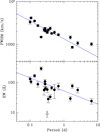 |
Fig. 3. Power-law fits to the orbital dependence of the FWHM and EW in quiescent BH XRTs. The EW of XTE J1650-400 (open circle) has been masked from the fit. |
The previous expressions provide rough estimates of BH orbital periods based on FWHM and EW information alone. We refer to these as PFWHM and PEW, respectively. Given the scatter in the power-law fits, the difference between these estimates and the true Porb can be significant. However, since both PFWHM and PEW are expected to track Porb better in BHs than in CVs, we decided to choose the ratio Pr ≡ (PFWHM/PEW)0.43 as a suitable metric for BH selection, which we now approximate as Pr ≈ 26 (EW/FWHM). Figure 4 depicts Pr against FWHM for our BHs and the ensemble of CVs.
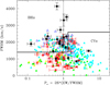 |
Fig. 4. Diagram showing the distribution of BHs and CVs in the FWHM-Pr plane. The same symbol code is used as in Figs. 1 and 2. Vertical dots mark the BH clustering line, while the thick solid lines delineate the optimal region for separating BHs from CVs. |
Since BHs are expected to cluster around Pr ≈ 1, it thus seems convenient to choose vertical bands of different widths, centred at Pr = 1, to optimise their selection against CVs. As is shown in Table 2, the narrower the band the more CVs are rejected, but this comes at the cost of selecting fewer BHs too. Interestingly, the distribution of BHs appears to be skewed towards lower Pr values, with very few BHs also found under FWHM = 1400 km s−1. Furthermore, dynamical arguments based on the Chandrasekhar mass limit indicate that CVs cannot produce Hα lines broader than ≃2600 km s−1 (see Fig. 1, also C15). Given the above constraints, we propose an optimal region for BH selection defined by the limits FWHM > 1400 km s−1 for Pr < 1.35 and FWHM > 2600 km s−1 for Pr > 1.35. These cuts are shown in Figure 4 and allow one to select 80% of the current sample of BHs, while rejecting 77% of the CVs. It is worth noting that at least 33% of the non-rejected CVs are eclipsing3 and therefore easily identified by light curve variability. It should also be mentioned that the mere detection of eclipses provides us with Porb information and thus, when combined with FWHM values, mass functions that constrain the nature of the compact star.
BH selection against CV rejection using the Pr metric.
Figure 5 displays the Pr metric in the simpler EW-FWHM plane. Here the BHs tend to cluster around FWHM/EW = 26 (dotted line in Fig. 5), while the previous selection cuts are represented by the solid lines defined by
 (1)
(1)
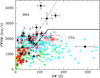 |
Fig. 5. Distribution of BHs and CVs in the FWHM-EW plane. The BH clustering line at FWHM = 26 × EW is indicated by dots, while the solid line marks our Fig. 4 cuts for optimal BH selection. |
with the FWHM expressed in units of kilometers per second and EW in angstroms.
Obviously, the proposed cuts are based on a limited number of BHs and should be considered as preliminary. In any case, they can help to discover new dormant BHs under the FWHM ≈ 2200 km s−1 limit proposed in C18. The diagnostics presented here will prove useful for current and future synoptic spectroscopic surveys (e.g. LAMOST, 4MOST, WEAVE), in which large numbers of spectra will be collected. It will also benefit blind photometric surveys, such as HαWKs and its pathfinder (Mini-HαWKs), which have been tailored to extract EW and FWHM information from Hα-emitting objects (C18). Nevertheless, CVs have an estimated Galactic density of ∼104 kpc−3 (Pala et al. 2020) and are thus ≈1000 times more abundant than BH XRTs (Corral-Santana et al. 2016). This implies that, assuming similar absolute magnitudes and galactic distributions, our FWHM-EW cuts would still select ≈300 intruding CVs per BH. Clearly, additional information from other multi-frequency surveys will be crucial for unveiling BH imposters and refining selection diagnostics. In particular, the absence of blue/UV excess in UVEX/Galex colours (a signature of a white dwarf or disc boundary layer; e.g. Gänsicke et al. 2009), will strengthen the possibility that new candidates are authentic dormant BH XRTs. Ultimately, these will need to be confirmed by dedicated follow-up spectroscopic studies.
A related question is whether FWHM and/or EW information can be used to distinguish BH XRTs that are undergoing some level of accretion activity from truly quiescent systems, even if X-rays are not detected. BH XRTs are known to follow a distinct FWHM and EW pattern as they transition from outburst to quiescence. Many examples in the literature consistently show that outburst spectra evolve from being almost featureless (sometimes with weak Hα emission embedded in broad absorptions) to developing increasingly stronger and broader Hα lines. For example, during the decay of the A0620-00 discovery outburst, the EW increased from ∼5.8 to 14 Å and FWHM from ∼1100 to 1830 km s−1 between Sept. 1975 and May 1976 (Whelan et al. 1977). Other studies, focusing on the late outburst decline, suggest that the FWHM tends to approach quiescent values faster than the EW. For example, from November 2000 to April 2001, XTE J1118+480 promptly reached the quiescent FWHM value at ≃2700 km s−1, while the EWs showed a monotonic increase between 14 and 44 Å, still far from the ≃87 Å quiescent value (Zurita et al. 2002a; Torres et al. 2004). In view of this, it seems tempting to conclude that Hα EWs are a more sensitive diagnostic of disc activity than FWHMs and could perhaps be used to detect unusual disc activity or even precursors to new outbursts. Interestingly, a chance spectrum of V404 Cyg obtained 13 h before the X-ray trigger of the 2015 outburst revealed that the EW of the Hα line was ∼15 times larger than in quiescence, while the FWHM was almost unchanged (Bernardini et al. 2016; Casares et al. 2019).
4. Conclusions
-
We have compiled FWHM and EW values of Hα emission lines in a sample of 20 quiescent BH XRTs. The BH collection typically covers multiple epochs of quiescence, sometimes spanning several decades. Despite evidence of orbital and secular variability, the mean FWHM and EW values are found to be rather stable (Appendix A). The BH FWHM and EW values have been compared with the ones of a sample of 353 CVs (305 from SDSS I to IV) with known orbitalperiods.
-
Our compilation shows that both FWHM and EW values decrease with Porb, while, for a given Porb, they tend to be larger in BHs than in CVs.
-
The larger BH FWHMs are a natural consequence of their higher compact object masses. The larger EWs, on the other hand, could be explained by a lower level of continuum flux. This stems from a combination of extreme mass ratios (which limit the relative contribution of the companion to the total flux) and the absence of a white dwarf continuum.
-
Furthermore, we derive an empirical Porb − Teff relation for companion stars in BH XRTs, which is also valid for CVs (Appendix B). From this we infer that the companion is the main source of Hα continuum flux above ≃0.2 d, while the accretion disc dominates otherwise. In the case of CVs, the white dwarf also contributes to the diluting continuum (especially at Porb ≲ 0.085 d), further capping EW values with respect to BHs.
-
We finally present a tentative metric (Pr = 26 EW/FWHM) for detecting dormant BHs, based on the period dependence of the FWHM and EW in BH XRTs. We find that selection cuts defined by FWHM > 1400 km s−1 for Pr < 1.35 and FWHM > 2600 km s−1 for Pr > 1.35 allow us to filter out ≈77% of CVs, while still retaining ≈80% of our sample of BHs. In any case, given the high Galactic density of CVs, the proposed metric needs to be combined with other multi-frequency diagnostics for an efficient selection of dormant BH XRTs.
We consider dormant BHs to be quiescent BH XRTs that will eventually trigger an outburst episode. Therefore, we will hereafter use the terms, ‘dormant’ and ‘quiescent’ interchangeably.
Photometry performed on the acquisition image indicates that the system was 1.4 mags brighter than quiescence at the time of the spectroscopic observations (see Appendix A for details). Assuming a constant Hα flux, this would imply that the quoted EW is underestimated by a factor of ≈3.6.
Other non-rejected SDSS CVs may also be eclipsing, but have not yet been confirmed due to insufficient photometric coverage.
Images are publicly available at http://decaps.skymaps.info/
Molly was written by T. R. Marsh and is available from https://cygnus.astro.warwick.ac.uk/phsaap/software/molly/html/INDEX.html.
In semi-detached binaries with an accreting compact star a hot-spot is formed by the collision of the gas stream with the outer accretion disc. For extreme mass ratios, characteristic of BH XRTs, the hot-spot crosses the observer’s line of sight at orbital phases ≃0.4 and 0.9, with phase 0 defined as the inferior conjunction of the mass donor star.
Acknowledgments
We thank the anonymous referee for useful and constructive comments that helped improve the manuscript. JC and MAPT acknowledge support by the Spanish Ministry of Science via the Plan de Generación de Conocimiento through grants PID2022-143331NB-100 and PID2021-124879NB-I00, respectively. SNU is supported by the FPI grant PREP2022-000508, also under program PID2022-143331NB-100. We thank Keith Inight for sharing his database of SDSS CV spectra with us, and Cynthia Froning for sharing the SED data on A0620-00. We also thank Rosa Clavero, David Jones and other members of the IAC team of support astronomers for undertaking the 2016-2021 NOT observations of V404 Cyg during Service time. We dedicate this paper to the memory of Tom Marsh, creator of the molly software and a beacon in the field of compact binaries.
References
- Abbott, B. P., Abbott, R., Abbott, T. D., et al. 2019, ApJ, 882, L24 [Google Scholar]
- Arur, K., & Maccarone, T. J. 2018, MNRAS, 474, 69 [Google Scholar]
- Baglio, M. C., Russell, D. M., Alabarta, K., et al. 2023, ATel., 16192, 1 [Google Scholar]
- Beer, M. E., & Podsiadlowski, P. 2002, MNRAS, 331, 351 [NASA ADS] [CrossRef] [Google Scholar]
- Bellm, E. C., Wang, Y., van Roestel, J., et al. 2023, ApJ, 956, 21 [Google Scholar]
- Bernardini, F., Russell, D. M., Shaw, A. W., et al. 2016, ApJ, 818, L5 [NASA ADS] [CrossRef] [Google Scholar]
- Bertelli, G., Girardi, L., Marigo, P., & Nasi, E. 2008, A&A, 484, 815 [NASA ADS] [CrossRef] [EDP Sciences] [Google Scholar]
- Bertelli, G., Nasi, E., Girardi, L., & Marigo, P. 2009, A&A, 508, 355 [NASA ADS] [CrossRef] [EDP Sciences] [Google Scholar]
- Burdge, K. B., El-Badry, K., Kara, E., et al. 2024, Nature, 635, 316 [NASA ADS] [CrossRef] [Google Scholar]
- Buxton, M., & Vennes, S. 2001, PASA, 18, 91 [Google Scholar]
- Callanan, P. J., & Charles, P. A. 1991, MNRAS, 249, 573 [Google Scholar]
- Calvelo, D. E., Vrtilek, S. D., Steeghs, D., et al. 2009, MNRAS, 399, 539 [Google Scholar]
- Cantrell, A. G., Bailyn, C. D., McClintock, J. E., & Orosz, J. A. 2008, ApJ, 673, L159 [Google Scholar]
- Cantrell, A. G., Bailyn, C. D., Orosz, J. A., et al. 2010, ApJ, 710, 1127 [NASA ADS] [CrossRef] [Google Scholar]
- Casares, J. 1996, in Proc. of the 158th coll. of IAU, eds. A. Evans, & J. H. Wood (Dordrecht: Kluwer Academic Publishers), Astrophys. Space Sci. Lib., 208, 395 [Google Scholar]
- Casares, J. 2015, ApJ, 808, 80 [NASA ADS] [CrossRef] [Google Scholar]
- Casares, J. 2016, ApJ, 822, 99 [NASA ADS] [CrossRef] [Google Scholar]
- Casares, J. 2018, MNRAS, 473, 5195 [CrossRef] [Google Scholar]
- Casares, J., & Charles, P. A. 1994, MNRAS, 271, L5 [NASA ADS] [CrossRef] [Google Scholar]
- Casares, J., & Torres, M. A. P. 2018, MNRAS, 481, 4372 [Google Scholar]
- Casares, J., Charles, P. A., Naylor, T., & Pavlenko, E. P. 1993, MNRAS, 265, 834 [Google Scholar]
- Casares, J., Charles, P. A., & Marsh, T. R. 1995a, MNRAS, 277, L45 [Google Scholar]
- Casares, J., Martin, A. C., Charles, P. A., et al. 1995b, MNRAS, 276, L35 [NASA ADS] [Google Scholar]
- Casares, J., Martín, E. L., Charles, P. A., Molaro, P., & Rebolo, R. 1997, New Astron., 1, 299 [NASA ADS] [CrossRef] [Google Scholar]
- Casares, J., Zurita, C., Shahbaz, T., Charles, P. A., & Fender, R. P. 2004, ApJ, 613, L133 [Google Scholar]
- Casares, J., Orosz, J. A., Zurita, C., et al. 2009, ApJS, 181, 238 [NASA ADS] [CrossRef] [Google Scholar]
- Casares, J., Muñoz-Darias, T., Mata Sánchez, D., et al. 2019, MNRAS, 488, 1356 [NASA ADS] [CrossRef] [Google Scholar]
- Casares, J., Torres, M. A. P., Muñoz-Darias, et al. 2022, MNRAS, 516, 2023 [NASA ADS] [CrossRef] [Google Scholar]
- Casares, J., Yanes-Rizo, I. V., Torres, M. A. P., et al. 2023, MNRAS, 526, 5209 [NASA ADS] [CrossRef] [Google Scholar]
- Chevalier, C., Ilovaisky, S. A., Leisy, P., & Patat, F. 1999, A&A, 347, L51 [NASA ADS] [Google Scholar]
- Ciatti, F., & Vittone, A. 1977, IBVS N. 1261 [Google Scholar]
- Corral-Santana, J. M., Casares, J., Shahbaz, T., et al. 2011, MNRAS, 413, L15 [NASA ADS] [Google Scholar]
- Corral-Santana, J. M., Casares, J., Muñoz-Darias, T., et al. 2013, Science, 339, 1048 [NASA ADS] [CrossRef] [Google Scholar]
- Corral-Santana, J. M., Casares, J., Muñoz-Darias, T., et al. 2016, A&A, 587, A61 [NASA ADS] [CrossRef] [EDP Sciences] [Google Scholar]
- Corral-Santana, J. M., Torres, M. A. P., Shabaz, T., et al. 2018, MNRAS, 475, 1036 [NASA ADS] [CrossRef] [Google Scholar]
- Drilling, J. S., & Landolt, A. U. 2002, in Allen’s Astrohysical Quantities, ed. A. N. Cox (New York, NY: Springer), Normal Stars, 381 [Google Scholar]
- Eggleton, P. P. 1983, ApJ, 268, 368 [Google Scholar]
- Filippenko, A. V., Matheson, T., & Barth, A. J. 1995, ApJ, 455, L139 [NASA ADS] [Google Scholar]
- Filippenko, A. V., Leonard, D. C., Matheson, T., et al. 1999, PASP, 111, 969 [Google Scholar]
- Frank, J., King, A. R., & Raine, D. J. 2002, Accretion Power in Astrophysics, 3rd ed. (Cambridge: Cambridge Univ. Press), 21 [Google Scholar]
- Froning, C. S., Robinson, E. L., & Bitner, M. A. 2007, ApJ, 663, 1215 [Google Scholar]
- Froning, C. S., Cantrell, A. G., Maccarone, T. J., et al. 2011, ApJ, 743, 26 [Google Scholar]
- Gaia Collaboration (Panuzzo, P., et al.) 2024, A&A, 686, L2 [NASA ADS] [CrossRef] [EDP Sciences] [Google Scholar]
- Gandhi, P., Rao, A., Johnson, M. A. C., Paice, J. A., & Maccarone, T. J. 2019, MNRAS, 485, 2642 [Google Scholar]
- Gandhi, P., Rao, A., Charles, P. A., et al. 2020, MNRAS, 496, L22 [NASA ADS] [CrossRef] [Google Scholar]
- Gänsicke, B. T., Dillon, M., Southworth, J., et al. 2009, MNRAS, 397, 2170 [NASA ADS] [CrossRef] [Google Scholar]
- Garcia, M. R., & Wilkes, B. J. 2002, ATel., 104, 1 [Google Scholar]
- Garcia, M. R., Callanan, P. J., McClintock, J. E., & Zhao, P. 1996, ApJ, 460, 932 [Google Scholar]
- Gelino, D. M., & Harrison, T. E. 2003, ApJ, 599, 1254 [Google Scholar]
- Gelino, D. M., Harrison, T. E., & Orosz, J. A. 2001, AJ, 122, 2668 [Google Scholar]
- Gelino, D. M., Balman, Ş., Kiziloğlu, Ü., et al. 2006, ApJ, 642, 438 [Google Scholar]
- González Hernández, J. I., & Casares, J. 2010, A&A, 516, A58 [NASA ADS] [CrossRef] [EDP Sciences] [Google Scholar]
- González Hernández, J. I., Rebolo, R., Israelian, G., et al. 2004, ApJ, 609, 988 [Google Scholar]
- González Hernández, J. I., Rebolo, R., Israelian, G., et al. 2006, ApJ, 644, L49 [Google Scholar]
- González Hernández, J. I., Rebolo, R., Israelian, G., et al. 2008a, ApJ, 679, 732 [Google Scholar]
- González Hernández, J. I., Rebolo, R., & Israelian, G. 2008b, A&A, 478, 203 [NASA ADS] [CrossRef] [EDP Sciences] [Google Scholar]
- González Hernández, J. I., Casares, J., Rebolo, R., et al. 2011, ApJ, 738, 95 [CrossRef] [Google Scholar]
- González Hernández, J. I., Rebolo, R., & Casares, J. 2012, ApJ, 744, L25 [CrossRef] [Google Scholar]
- González Hernández, J. I., Rebolo, R., & Casares, J. 2014, MNRAS, 438, L21 [CrossRef] [Google Scholar]
- González Hernández, J. I., Suárez-Andrés, L., Rebolo, R., & Casares, J. 2017, MNRAS, 465, L15 [CrossRef] [Google Scholar]
- Harlaftis, E. T., & Greiner, J. 2004, A&A, 414, L13 [NASA ADS] [CrossRef] [EDP Sciences] [Google Scholar]
- Harlaftis, E. T., Horne, K., & Filippenko, A. V. 1996, PASP, 108, 762 [Google Scholar]
- Harlaftis, E. T., Steeghs, D., Horne, K., & Filippenko, A. V. 1997, AJ, 114, 1170 [Google Scholar]
- Harlaftis, E. T., Collier, S., Horne, K., & Filippenko, A. V. 1999, A&A, 341, 491 [Google Scholar]
- Harrison, T. E., Howell, S. B., Szkody, P., & Cordova, F. A. 2007, AJ, 133, 162 [NASA ADS] [CrossRef] [Google Scholar]
- Haswell, C. A., Hynes, R. I., King, A. R., & Schenker, K. 2002, MNRAS, 332, 928 [Google Scholar]
- Heida, M., Jonker, P. G., Torres, M. A. P., & Chiavassa, A. 2017, ApJ, 846, 132 [Google Scholar]
- Hynes, R. I., & Robinson, E. L. 2012, ApJ, 749, 3 [Google Scholar]
- Hynes, R. I., Zurita, C., Haswell, C. A., et al. 2002, MNRAS, 330, 1009 [NASA ADS] [CrossRef] [Google Scholar]
- Hynes, R. I., Charles, P. A., Garcia, M. R., et al. 2004, ApJ, 611, L125 [Google Scholar]
- Hynes, R. I., Bradley, C. K., Rupen, M., et al. 2009, MNRAS, 399, 2239 [Google Scholar]
- Inight, K., Gänsicke, B. T., Breedt, E., et al. 2023, MNRAS, 524, 4867 [NASA ADS] [CrossRef] [Google Scholar]
- Israelian, G., Rebolo, R., Basri, G., Casares, J., & Martín, E. L. 1999, Nature, 401, 142 [Google Scholar]
- Jonker, P. G., Kaur, K., Stone, N., & Torres, M. A. P. 2021, ApJ, 921, 131 [NASA ADS] [CrossRef] [Google Scholar]
- Khargharia, J., Froning, C. S., & Robinson, E. L. 2010, ApJ, 716, 1105 [NASA ADS] [CrossRef] [Google Scholar]
- Khargharia, J., Froning, C. S., Robinson, E. L., & Gelino, D. M. 2013, AJ, 145, 21 [NASA ADS] [CrossRef] [Google Scholar]
- King, A. R. 1993, MNRAS, 260, L5 [Google Scholar]
- King, A. R., Kolb, U., & Burderi, L. 1996, ApJ, 464, L127 [NASA ADS] [CrossRef] [Google Scholar]
- King, N. L., Harrison, T. E., & McNamara, B. J. 1996, AJ, 111, 1675 [Google Scholar]
- Knevitt, G., Wynn, G. A., Vaughan, S., & Watson, M. G. 2014, MNRAS, 437, 3087 [Google Scholar]
- Knigge, C. 2006, MNRAS, 373, 484 [NASA ADS] [CrossRef] [Google Scholar]
- Koljonen, K. I. I., Russell, D. M., Corral-Santana, J. M., et al. 2016, MNRAS, 460, 942 [Google Scholar]
- Kreidberg, L., Bailyn, C. D., Farr, W., & Kalogera, V., 2012, ApJ, 757, 36 [NASA ADS] [CrossRef] [Google Scholar]
- Kuulkers, E., Kouveliotou, C., Belloni, T., et al. 2013, A&A, 552, A32 [NASA ADS] [CrossRef] [EDP Sciences] [Google Scholar]
- Lin, J., Yan, Z., Han, Z., & Yu, W., 2019, ApJ, 870, 126 [Google Scholar]
- Littlefair, S., Dhillon, V. S., Marsh, T. R., & Gänsicke, B. T. 2006, MNRAS, 371, 1435 [Google Scholar]
- Maccarone, T. J., & Patruno, A. 2013, MNRAS, 428, 1335 [Google Scholar]
- Macias, P., Orosz, J. A., Bailyn, C. D., et al. 2011, BAAS, 43, 2011 [Google Scholar]
- Marsh, T. R., Robinson, E. L., & Wood, J. H. 1994, MNRAS, 266, 137 [NASA ADS] [CrossRef] [Google Scholar]
- Mata Sánchez, D., Muñoz-Darias, T., Casares, J., Corral-Santana, J. M., & Shahbaz, T. 2015, MNRAS, 454, 2199 [CrossRef] [Google Scholar]
- Mata Sánchez, D., Muñoz-Darias, T., Casares, J., & Jiménez Ibarra, F. 2017, MNRAS, 464, L41 [CrossRef] [Google Scholar]
- Mata Sánchez, D., Rau, A., Álvarez-Hernández, A., et al. 2021, MNRAS, 506, 581 [CrossRef] [Google Scholar]
- McClintock, J. E., & Remillard, R. A. 1986, ApJ, 308, 110 [Google Scholar]
- McClintock, J. E., Horne, K., & Remillard, R. A. 1995, ApJ, 442, 358 [Google Scholar]
- McClintock, J. E., Garcia, M. R., Caldwell, N., et al. 2001, ApJ, 551, L147 [Google Scholar]
- McClintock, J. E., Narayan, R., Garcia, M. R., et al. 2003, ApJ, 593, 435 [Google Scholar]
- Menou, K., Narayan, R., & Lasota, J.-P. 1999, ApJ, 513, 811 [Google Scholar]
- Murdin, P., Griffiths, R. E., Pounds, K. A., Watson, M. G., & Longmore, A. J. 1977, MNRAS, 178, 27 [Google Scholar]
- Murdin, P., Allen, D. A., Morton, D. C., Whelan, J. A. J., & Thomas, R. M. 1980, MNRAS, 192, 709 [Google Scholar]
- Naoz, S., Fragos, T., Geller, A., et al. 2016, ApJ, 822, L24 [NASA ADS] [CrossRef] [Google Scholar]
- Narayan, R., & McClintock, J. E. 2005, ApJ, 623, 1017 [Google Scholar]
- Neilsen, J., Steeghs, D., & Vrtilek, S. D. 2008, MNRAS, 384, 849 [Google Scholar]
- Oke, J. B. 1977, ApJ, 217, 181 [Google Scholar]
- Orosz, J. A. 2003, in A Massive Star Odyssey, from Main Sequence to Supernova, eds. K. van der Hucht, A. Herrero, & C. Esteban (San Francisco: Astronomical Society of the Pacific), Proc. of IAU Symp., 212, 3650 [Google Scholar]
- Orosz, J. A., & Bailyn, C. D. 1995, ApJ, 446, L59 [Google Scholar]
- Orosz, J. A., & Bailyn, C. D. 1997, ApJ, 477, 876 [Google Scholar]
- Orosz, J. A., Bailyn, C. D., Remillard, R. A., McClintock, J. E., & Foltz, C. B. 1994, ApJ, 436, 848 [NASA ADS] [CrossRef] [Google Scholar]
- Orosz, J. A., Bailyn, C. D., McClintock, J. E., & Remillard, R. A. 1996, ApJ, 468, 380 [NASA ADS] [CrossRef] [Google Scholar]
- Orosz, J. A., Jain, R. K., Bailyn, C. D., McClintock, J. E., & Remillard, R. A. 1998, ApJ, 499, 375 [NASA ADS] [CrossRef] [Google Scholar]
- Orosz, J. A., Kuulkers, E., van der Klis, M., et al. 2001, ApJ, 555, 489 [NASA ADS] [CrossRef] [Google Scholar]
- Orosz, J. A., Groot, P. J., van der Klis, M., et al. 2002, ApJ, 568, 845 [NASA ADS] [CrossRef] [Google Scholar]
- Orosz, J. A., McClintock, J. E., Remillard, R. A., & Corbel, S. 2004, ApJ, 616, 376 [NASA ADS] [CrossRef] [Google Scholar]
- Orosz, J. A., Steiner, J. F., McClintock, J. E., et al. 2011, ApJ, 730, 75 [NASA ADS] [CrossRef] [Google Scholar]
- Özel, F., Psaltis, D., Narayan, R., & McClintock, J. E. 2010, ApJ, 725, 1918 [CrossRef] [Google Scholar]
- Paczyński, B. 1971, ARA&A, 9, 183 [Google Scholar]
- Pala, A. F., Gänsicke, B. T., Breedt, E., et al. 2020, MNRAS, 494, 3799 [Google Scholar]
- Pecaut, M. J., & Mamajek, E. E. 2013, ApJS, 208, 9 [Google Scholar]
- Peterson, B. M., Ferrarese, L., Gilbert, K. M., et al. 2004, ApJ, 613, 682 [Google Scholar]
- Podsiadlowski, Ph., Rappaport, S., & Pfahl, E. D. 2002, ApJ, 565, 1107 [NASA ADS] [CrossRef] [Google Scholar]
- Podsiadlowski, Ph., Rappaport, S., & Han, Z. 2003, MNRAS, 341, 385 [NASA ADS] [CrossRef] [Google Scholar]
- Poutanen, J., Veledina, A., Berdyugin, A. V., et al. 2022, Science, 375, 874 [NASA ADS] [CrossRef] [Google Scholar]
- Pylyser, E., & Savonije, G. J. 1988, A&A, 191, 57 [Google Scholar]
- Remillard, R. A., McClintock, J. E., & Bailyn, C. D. 1992, ApJ, 399, L145 [Google Scholar]
- Remillard, R. A., Orosz, J. A., McClintock, J. E., & Bailyn, C. D. 1996, ApJ, 459, 226 [Google Scholar]
- Ritter, H., & Kolb, U. 2003, A&A, 404, 301 [NASA ADS] [CrossRef] [EDP Sciences] [Google Scholar]
- Ruiz, M., Shapiro, S. L., & Tsokaros, A. 2018, PhRvD, 97, 021501 [Google Scholar]
- Russell, D. M., Lewis, F., & Gandhi, P. 2017, ATel., 10797, 1 [Google Scholar]
- Russell, D. M., Qasim, A. A., Bernardini, F., et al. 2018, ApJ, 852, 90 [NASA ADS] [CrossRef] [Google Scholar]
- Saikia, P., Russel, D. M., Baglio, M. C., et al. 2022, ApJ, 932, 38 [NASA ADS] [CrossRef] [Google Scholar]
- Sánchez-Fernández, C., Zurita, C., Casares, J., et al. 2002, IAU Circ., 7989 [Google Scholar]
- Savoury, C. D. J., Littlefair, S. P., Dhillon, V. S., et al. 2011, MNRAS, 415, 2025 [Google Scholar]
- Shahbaz, T., van der Hooft, F., Charles, P. A., Casares, J., & van Paradijs, J. 1996, MNRAS, 282, L47 [Google Scholar]
- Shahbaz, T., Bandyopadhyay, R. M., & Charles, P. A. 1999a, A&A, 346, 82 [NASA ADS] [Google Scholar]
- Shahbaz, T., van der Hooft, F., Casares, J., Charles, P. A., & van Paradijs, J. 1999b, MNRAS, 306, 89 [Google Scholar]
- Shahbaz, T., Russell, D. M., Zuritas, C., et al. 2013, MNRAS, 434, 2696 [NASA ADS] [CrossRef] [Google Scholar]
- Shibata, M., Zhou, E., Kiuchi, K., et al. 2019, PhRvD, 100, 023015 [Google Scholar]
- Siegel, J. C., Kiato, I., Kalogera, V., et al. 2023, ApJ, 954, 212 [NASA ADS] [CrossRef] [Google Scholar]
- Smith, D. A., & Dhillon, V. S. 1998, MNRAS, 301, 767 [NASA ADS] [CrossRef] [Google Scholar]
- Steeghs, D., McClintock, J. E., Parsons, S. G., et al. 2013, ApJ, 768, 185 [Google Scholar]
- Thorstensen, J. R., Fenton, W. H., Patterson, J. O., et al. 2002a, ApJ, 567, L49 [NASA ADS] [CrossRef] [Google Scholar]
- Thorstensen, J. R., Fenton, W. H., Patterson, J. O., et al. 2002b, PASP, 114, 1117 [Google Scholar]
- Torres, M. A. P., Callanan, P. J., Garcia, M. R., et al. 2004, ApJ, 612, 1026 [NASA ADS] [CrossRef] [Google Scholar]
- Torres, M. A. P., Jonker, P. G., Miller-Jones, J. C. A., et al. 2015, MNRAS, 450, 4292 [NASA ADS] [CrossRef] [Google Scholar]
- Torres, M. A. P., Casares, J., Jiménez-Ibarra, F., et al. 2019, ApJ, 882, L21 [NASA ADS] [CrossRef] [Google Scholar]
- Torres, M. A. P., Casares, J., Jiménez-Ibarra, F., et al. 2020, ApJ, 893, L37 [NASA ADS] [CrossRef] [Google Scholar]
- Torres, M. A. P., Jonker, P. G., Casares, J., Miller-Jones, J. C. A., & Steeghs, D. 2021, MNRAS, 501, 2174 [NASA ADS] [CrossRef] [Google Scholar]
- van Belle, G. T., Lane, B. F., Thompson, R. R., et al. 1999, AJ, 117, 521 [NASA ADS] [CrossRef] [Google Scholar]
- Wagner, R. M., Foltz, C. B., Shahbaz, T., et al. 2001, ApJ, 556, 42 [Google Scholar]
- Webb, N. A., Naylor, T., Ioannou, Z., Charles, P. A., & Shahbaz, T. 2000, MNRAS, 317, 528 [Google Scholar]
- Webbink, R. F., Rappaport, S. A., & Savonije, G. J. 1983, ApJ, 270, 678 [NASA ADS] [CrossRef] [Google Scholar]
- Whelan, J. A. J., Ward, M. J., Allen, D. A., et al. 1977, MNRAS, 180, 657 [Google Scholar]
- Wu, Y. X., Yu, W., Li, T. P., Maccarone, T. J., & Li, X. D. 2010, ApJ, 718, 620 [Google Scholar]
- Wu, J., Orosz, J. A., McClintock, J. E., et al. 2015, ApJ, 806, 92 [NASA ADS] [CrossRef] [Google Scholar]
- Yanes-Rizo, I. V., Torres, M. A. P., Casares, J., et al. 2022, MNRAS, 517, 1476 [NASA ADS] [CrossRef] [Google Scholar]
- Yanes-Rizo, I. V., Torres, M. A. P., Casares, J., et al. 2024, MNRAS, 527, 5949 [Google Scholar]
- Yanes-Rizo, I. V., Torres, M. A. P., Casares, J., et al. 2025, A&A, 694, A119 [NASA ADS] [CrossRef] [EDP Sciences] [Google Scholar]
- Zhang, G., Russell, D. M., Bernardini, F., Gelfand, J. D., & Lewis, F. 2017, ATel., 10562, 1 [NASA ADS] [Google Scholar]
- Zheng, W.-M., Wu, Q., Wu, J., et al. 2022, ApJ, 925, 83 [Google Scholar]
- Zorotovic, M., Schreiber, M. R., & Gänsicke, B. T. 2011, A&A, 536, A42 [NASA ADS] [CrossRef] [EDP Sciences] [Google Scholar]
- Zurita, C., Casares, J., Shahbaz, T., et al. 2002a, MNRAS, 333, 791 [CrossRef] [Google Scholar]
- Zurita, C., Sánchez-Fernández, C., Casares, J., et al. 2002b, MNRAS, 334, 999 [Google Scholar]
- Zurita, C., Casares, J., Martínez-Pais, I. G., et al. 2002c, IAU Circ., 7868 [Google Scholar]
- Zurita, C., Torres, M. A. P., Steeghs, D., et al. 2006, ApJ, 644, 432 [Google Scholar]
- Zurita, C., Corral-Santana, J. M., & Casares, J. 2015, MNRAS, 454, 3351 [Google Scholar]
- Zurita, C., González Hernández, J. I., Escorza, A., & Casares, J. 2016, MNRAS, 460, 4289 [Google Scholar]
Appendix A: An extensive collection of FWHM and EW values of Hα lines in quiescent BH XRTs
We have assembled a new database of Hα spectra of quiescent BH XRTs obtained in different epochs over 30 years. The present collection contains and supersedes the one reported in C15 and is presented in Table A.1. Listed references correspond to the papers where the original spectra were first reported and/or analysed. The spectra were obtained with a variety of telescopes: the 10.4 m Gran Telescopio Canarias (GTC), the 10 m Keck telescope, the 8.2 m Very Large Telescope (VLT), the 6.5 m Magellan Clay telescope, the 4.2 m William Herschel Telescope (WHT), the 4 m Victor M. Blanco telescope, the 3.9 m Anglo Australian Telescope (AAT), the 3.5 m New Technology Telescope (NTT), the 2.5 m Isaac Newton Telescope (INT), the 2.56 m Nordic Optical Telescope (NOT) and the 2.1 m telescope at the Observatorio de San Pedro Mártir (SPM). Some data have not yet been published and will be reported elsewhere. These are the 2019-2021 NOT and 2022 INT epochs of V404 Cyg, the 2023 GTC epoch of MAXI J1820+070, the 2019 GTC epoch of XTE J1859+226 and the 2017 GTC epoch of GRO J0422+32.
We consider BH XRTs to be in true quiescence when there is no sign of X-ray activity (i.e. outbursts, mini-outbursts or reflares) and the optical flux remains consistent with the lowest measured values. To demonstrate that the selected spectra meet these criteria, we give in Table A.2 the dates of the quiescent periods relevant to our data. The listed magnitudes refer either to the start of quiescence, to a time average or to a range of values reported over the entire period. As can be seen in Table A.2, all the spectra correspond to quiescent epochs, including GX 339-4, which experienced a prolonged period of very low optical brightness in 2016 (Russell et al. 2017). The only exception is XTE J1650-500, as the spectroscopy of Sánchez-Fernández et al. (2002) was obtained approximately two months before the first quiescent magnitudes were reported (Garcia & Wilkes 2002). To confirm this, we have performed PSF photometry on the acquisition images obtained by Sánchez-Fernández et al. (2002), finding R = 20.67±0.04, i.e. 1.4 mag brighter than the deepestmagnitude available (Garcia & Wilkes 2002). To further test whether the latter corresponds to true quiescence, we also performed PSF photometry on a Sloan r-band image from the DECaPS survey4, obtained on 29 April 2017 under good seeing conditions (0.78"). We found r’ = 22.10±0.12, which is in good agreement with Garcia & Wilkes (2002).
Following C15, we measured the FWHM of the Hα line by fitting a Gaussian profile plus a constant in a window of ±10 000 km s−1 centred at 6563 Å, after masking the neighboring He I λ6678 line. The Gaussian model was previously degraded to the instrumental resolution of each spectrum, and the continuum level was rectified by fitting a low-order polinomial. Likewise, EW values were obtained by integrating the Hα flux in the continuum normalised spectra. The entire spectral analysis was performed using routines within the MOLLY package5. Where possible, FWHM and EW values were measured from single individual spectra (e.g. V404 Cyg). When the quality of individual spectra was too poor FWHM and EW measurements were obtained from averaged spectra (e.g. MAXI J1659-152). In some cases, an orbitally averaged spectrum was kindly provided by the corresponding authors (e.g. GX 339-4) while in others we had to digitise averaged spectra from figures in the relevant papers (e.g. the WHT 1991-1992 epoch of A0620-00). The uncertainties introduced by the latter process are negligible compared to orbital and long-term variations typically observed in FWHM and EW.
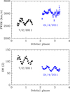 |
Fig. A.1. Orbital variation of FWHM and EW in XTE J1118+480 on the nights of February 7 and April 24 2011. |
Figure A.1 shows examples of orbital variability in the FWHM and EW values of XTE J1118+480 at two different epochs. Both parameters describe a double sine wave on each orbital cycle. The EW variations reflect changes in the optical continuum, driven by the ellipsoidal modulation of the companion star (e.g. Marsh et al. 1994). On the other hand, the phasing of the FWHM variations (i.e. minima at phases 0.4 and 0.9) indicate that these are likely caused by the motion of the hot-spot6 across the Hα profile. Consequently, when only one spectrum is available in a given epoch (e.g. the Keck 2004 spectrum of XTE J1118+480) or its phase coverage is very limited (e.g. the WHT 1993 epoch of V404 Cyg), statistical uncertainties in FWHM and EW measurements were increased by adding quadratically a systematic error to account for the effect of orbital variability. We call these ’orbital’ systematic errors σ(FWHM)orb and σ(EW)orb, respectively.
To estimate σ(FWHM)orb and σ(EW)orb, we focus on 24 epochs of 10 BHs with ≥50 % orbital coverage. In principle, one might expect σ(FWHM)orb and σ(EW)orb to depend on geometrical effects, different accretion disc structures or mass accretion rates. However, we see no evidence for a trend in the amplitude of the FWHM and EW variability with fundamental parameters such as binary inclination and Porb, a proxy for mass transfer rate. Conversely, Fig. A.2 shows that the amplitude of the variability increases with the mean value, with a linear fit giving σ(FWHM)orb = 0.05 FWHM and σ(EW)orb = 0.10 EW. Three epochs (the 2022 INT campaign on V404 Cyg, the 1995 WHT on GS2000+25 and the 2013 GTC on Swift J1357.2-0933) have significantly larger variability in FWHM than the remaining 21, but this is caused by statistical noise because the individual spectra in these campaigns have very poor signal-to-noise ratios S/N≲3 compared to the rest, which typically have S/N≳10. In any case, excluding these three epochs does not change the linear fits. The effect of these three epochs on the EW variability (which is an integrated line flux) is otherwise negligible, despite the poor quality of the spectra. On the basis of Fig. A.2, and in the absence of a better approach, we decided to adopt orbital fractional errors that are constant for all the systems, i.e. σ(FWHM)orb/FWHM = 0.05 and σ(EW)orb/EW = 0.10.
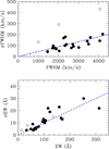 |
Fig. A.2. Orbital variability of FWHM (upper panel) and EW (lower panel) for 24 epochs of 10 BH XRTs with ≥50% orbital coverage. Open circles mark the three epochs with S/N≲3 spectra and thus dominated by statistical noise. The dashed blue lines show linear fits to the data. |
Figure A.1 also depicts clear changes in the FWHM and EW mean values from epoch to epoch. These might be caused by geometric changes in a precessing accretion disc (see Zurita et al. 2002a, Torres et al. 2004, Calvelo et al. 2009, Zurita et al. 2016), although stronger support is needed for confirmation. Alternative explanations, such as fluctuations in the mass accretion rate, may also be responsible. For example, Cantrell et al. (2008) has shown that quiescent BH XRTs can sometimes transition between different optical states with distinct associated levels of aperiodic variability. In addition, a long-term brightening of the optical continuum has been reported in several XRTs, possibly caused by matter accumulating in the disc between outbursts (see Russell et al. 2018 and included references).
To quantify the long-term variations in FWHM and EW we have calculated the standard deviation of orbitally averaged measurements in 9 BHs with ≥25 % phase coverage spanning at least 3 different epochs. Figure A.3, for example, shows the secular FWHM and EW variability of a sample of BH XRTs through different epochs. The small sample size does not allow a detailed analysis, although the plot suggests that there is a stable mean value for each system with superimposed secular variability. The amplitude of the variability also appears to increase with the mean, so we again assume that a constant fractional variability can be adopted for all the systems. The average fractional standard deviation of the 9 BHs is σ(FWHM)sec = 0.04 FWHM and σ(EW)sec = 0.13 EW. We consider these as a new source of systematic error that need to be added quadratically to FWHM and EW measurements obtained from single-epoch data (e.g. N. Vel 93).
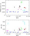 |
Fig. A.3. Long-term (secular) variation of FWHM and EW in a sample of quiescent BH XRTs. The plot covers a period of 30 years. Every point represents an orbital average over a single epoch. The color code is as follows: blue (V404 Cyg), cyan (GRO J0422+32), magenta (N. Mus 91), red (XTE J1859+226), black (XTE J1118+480) and green (SWIFT J1357.2-0933). |
The FWHM and EW values given for each epoch in Table A.1 do include the above systematic orbital and secular uncertainties, where necessary. With these new added systematic uncertainties, we have calculated the mean and standard deviation in the distribution of individual FWHM and EW values for each of the 20 BH XRTs. These are the final numbers listed in Table 1 and used in the main body of the paper.
Multi-epoch FWHM and EW of Hα lines in quiescent BH XRTs
Quiescent epochs and magnitudes
Appendix B: Empirical Porb − Teff relation for low-mass donors in BH X-ray transients
In order to derive an empirical Porb − Teff relation for donor stars in BH XRTs we start by collecting spectral types from the literature. The compilation is divided into two categories: low-mass companions M2≲1.5 M⊙ and intermediate-mass companions M2 ≈ 2 − 5 M⊙. The motivation for doing so is two-fold. On the one hand, XRTs with intermediate-mass companions (IMXBs) are thought to be precursors of those with low-mass companions (LMXBs), and thus represent a different evolutionary phase (Podsiadlowski et al. 2003). On the other, high luminosity donors in IMXBs totally veil disc emission lines, such as Hα, and, hence, are of little interest in the context of this paper. We therefore focus here on the group of BH LMXBs (Table B.1), although information on BH IMXBs is also provided for completeness (Table B.2). The categorisation of BW Cir is somewhat controversial because its donor is an early G-type star with a mass of ≈1 − 2.4 M⊙ that sits within the Hertzsprung gap (Casares et al. 2004). However, because of its moderately strong Hα line, we tentatively consider BW Cir as a BH LMXB in this work.
Reported spectral types have been determined following three different methods: (1) a qualitative classification, based on the presence (or lack thereof) of distinct spectral features (e.g. the G-band at ∼4310 Å, the Mg Ib triplet at ∼5170 Å, TiO or CO molecular bands, etc.), either in the visible (VIS SPEC) or near-infrared (NIR SPEC) part of the spectrum. In some cases, the classification is more quantitative as it relies on figures of merit such as the intensity of the highest cross-correlation peak or a χ2 minimisation of residuals after template subtraction. (2) Model fits to the observed (donor’s dominated) multi-wavelength spectral energy distribution (SED). (3) a direct Teff determination derived by fitting libraries of synthetic stellar models (SPEC FIT).
In the case of VIS/NIR SPEC and SED methods we transformed spectral types into Teff values. To do so we assume that LMXB donors below the bifurcation period (Porb≲18 h; see Podsiadlowski et al. 2002) can be approximated by main sequence (MS) stars and, thus, adopt the Teff scale from the empirical collection of table 5 in Pecaut & Mamajek (2013). For long period LMXBs (Porb≳3 d) we follow instead the Teff scale of giant stars from van Belle et al. (1999). Finally, LMXB donors with 18 h ≲Porb≲ 3 d are considered subgiants, and their Teff values interpolated between the MS and giant scales of Pecaut & Mamajek (2013) and van Belle et al. (1999).
To verify the reliability of these assumptions we have compared average densities ⟨ρ⟩ of LMXB companions with those of MS and giants stars of similar spectral types. The density of a Roche-lobe filling star is obtained by bringing the Roche lobe geometry into Kepler’s third law. Adopting Paczyński’s approximation for the volume-averaged Roche-lobe radius (Paczyński 1971) allows cancelling out the dependence on binary mass ratio q, leading to  , where Porb is given in units of hours and ⟨ρ⟩ in gr cm−3 (Frank et al. 2002). If instead we use Eggleton’s more accurate approximation (Eggleton 1983), we find
![Mathematical equation: $$ \begin{aligned} \langle \rho \rangle = 92.6 \times \frac{\left[0.6~q^{2/3} + \ln \left( 1+q^{1/3} \right) \right]^{3} }{q~\left( 1+q \right) }\times P_{\rm orb}^{-2},\, \end{aligned} $$](/articles/aa/full_html/2025/08/aa53935-25/aa53935-25-eq7.gif) (B.1)
(B.1)
equation that weakly depends on q. We note the former expression  is recovered for q = 0.22, which seems apropriate for cataclysmic variables. BH LMXBs, on the other hand, have more extreme mass ratios, with typical values q ≃ 0.06 (cf Casares 2016), leading to
  . Table B.3 presents an up-to-date collection of mass ratios in BH LMXBs and implied donor densities, according to eq. B.1. In any case, it should be noted that the use of Paczyński’s approximation is equally valid as it leads to tiny differences in density on the order of ≈2-4 %. A direct comparison with MS and giant star densities supports our choice of Teff scales for LMXB donors i.e. average donor densities above Porb≳3 d are in the range of giant stars while those with Porb≲18 h are consistent with typical MS or slightly evolved (i.e. oversized) stars.
Tables B.1 and B.2 summarise the spectral types collected from the literature and their associated Teff numbers. When several Teff values are present for a given system, the average (marked in bold) is selected. This was computed as the unweighted mean after randomising the individual (independent) measurements. Here we have assumed flat probability distributions for all methods except SPEC FIT, where a normal distribution is adopted. The evolution of Teff with Porb is presented in Fig. B.1. For reference, we also plot Porb − Teff tracks for MS and terminal age main sequence (TAMS) stars that would fit in their corresponding Roche lobes. To do so, we used eq. B.1 with q = 0.06 and mass-radius and mass-Teff relations for MS (Pecaut & Mamajek 2013) and TAMS (Bertelli et al. 2008, 2009). In addition, we depict stripped-giant models to track the location of low-mass donors that have evolved off the MS. The radius and luminosity (and thus Teff) of stripped-giant stars are uniquely determined by the mass of the degenerate helium core mc, which is constrained between the total stellar mass M2 and the Schönberg-Chandrasekhar limit ∼0.17M2 (Webbink et al. 1983; King 1993). Both models, mc = 0.17M2 (lower line) and mc = M2 (upper line), are displayed.
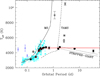 |
Fig. B.1. Observed Teff vs orbital period (Porb) for donor stars in BH XRTs. Asterisks indicate ≈2 − 5 M⊙ donor stars (IMXBs) while solid black circles low-mass ≲1.5 M⊙ donors (LMXBs). The open circles mark the position of the early G-type donor in BW Cir and the nuclear-evolved companion in XTE J1118+480. Solid triangles in cyan indicate donor stars in CVs from the compilation of Knigge (2006). The blue open triangles indicate the three nuclear-evolved donors in EI Psc, QZ Ser and SDSS 1702+3229. The red line shows our empirical fit to the group of CVs and BH LMXBs, excluding BW Cir and the nuclear-evolved companions in XTE J1118+480 and the three CVs. For comparison, we also plot Teff tracks of main sequence (MS), terminal age main sequence (TAMS) and stripped-giant stars that would fill the Roche lobes for a given Porb. |
Spectral types and Teff of donor stars in BH LMXBs
Spectral types and Teff of donor stars in BH IMXBs
Donor star densities in BH LMXBs (marked in bold), compared to those of MS and Giants with same spectral type.
Figure B.1 shows that LMXB donors with Porb≳1.5 d have crossed the TAMS line and follow the stripped-giant branch, while those with Porb≲1.5 d have not left the MS. In particular, donors with Porb≲ 0.3 d ( = 7 h) are only slightly evolved compared to MS stars on the empirical track of Pecaut & Mamajek (2013). XTE J1118+480 is a clear outlier since it is ∼500 K hotter than expected for a MS at its orbital period. This is reminiscent of the cataclysmic variables QZ Ser, EI Psc and SDSS J1702+3229, whose donors are thought to descend from more massive progenitors that were significantly evolved at the onset of mass transfer (Thorstensen et al. 2002a,b; Littlefair et al. 2006). Interestingly, XTE J1118+480 has shown evidence for CNO processed material, in support for a highly evolved donor progenitor (Haswell et al. 2002).
Overall, LMXB donors are seen to follow a well-defined path in the Porb − Teff plane. Unfortunately, this is weakly constrained at short orbital periods ≲0.14 d due to lack of data. To compensate for this we decided to include an updated collection of CV donor spectral types from Knigge (2006). These have been converted to Teff values, as was previously done for BH LMXBs. The addition of CV information seems justified, since previous work has shown that, for the same orbital period, donor stars in CVs and LMXBs are almost indistinguishable (e.g. Smith & Dhillon 1998).
In order to characterise the Teff evolution with Porb we fit the ensamble of BH LMXB and CV data points in three different regions: (i) short-periods below the period gap Porb ≤ 0.085 d (ii) intermediate-periods 0.085 d ≤Porb ≤ 0.2 d and (iii) long-periods Porb ≥ 0.2 d. We find that a broken power-law provides a good description of the long-period systems, while simple linear fits are used for shorter periods i.e.
 (B.2)
(B.2)
These empirical fits are represented by the red line in Fig. B.1. For the reasons given above, the five outliers (BW Cir, XTE J1118+480 plus the three CVs with confirmed nuclear-evolved donors) were masked in the fits. We note, however, that their inclusion does not significantly alter the results of the fits.
The surprisingly narrow path traced by LMXB donors in the Porb − Teff plane suggests that they all follow the same evolutionary track. King et al. (1996) showed that systems with Porb≲2 d evolve towards shorter periods because angular momentum losses shrink the binary orbit faster than stellar expansion. Conversely, for Porb≳2 d the companion is nuclear-evolved before the onset of mass transfer and the binary evolves to increasing orbital periods (see also Pylyser & Savonije 1988). The gap seen at ≃0.7 − 1.5 d thus reflects a real shortage of systems triggered by the bifurcation period, which causes binaries to evolve towards either shorter or longer Porb. In addition, the small scatter seen at periods ≈0.25-1 d implies that the orbital separation after common envelope ejection must have been sufficiently tight for the donor stars to come into contact before evolving significantly. To obtain a better description of the Porb − Teff relation for BH LMXBs at very short orbital periods ≲0.15 d, it would be important to determine spectral types for the donor stars in Swift J1357.2-0933 (0.12 d) and MAXI J1659-152 (0.10 d). This will require infrared spectroscopy since these stars are too cold to be detected at visible wavelengths (Mata Sánchez et al. 2015; Torres et al. 2015, 2021).
Appendix C: A simulation of Hα EWs in quiescent BH X-ray transients
We have built a toy model to simulate the EW of the Hα emission in quiescent BH XRTs. We assume typical BH XRT parameters, with a compact object mass M1 = 8 M⊙ and mass ratio q = 0.06. The binary separation is set by Kepler’s Third law  and the size of the secondary star by the effective Roche lobe radius through Eggleton’s approximation R2/a = 0.49 q2/3/[(0.6 q2/3+ln(1+q2/3)] (Eggleton 1983). The accretion disc is simulated by a flat cylinder truncated at the 3:1 resonance radius rd/a = (1/3)2/3(1 + q)−1/3 (Frank et al. 2002). Based on observations of extreme wing velocities in Hα profiles we set the inner disc radius at rin = 0.06rd (Casares et al. 2022), although this parameter has very little impact on the results of the simulation.
To estimate the EW of the Hα line we start by computing the continuum emitted by the secondary star and the accretion disc using blackbody approximations. The flux density radiated by the secondary star, fs(λ), is obtained from a blackbody with radius R2 and temperature Teff, where Teff depends on Porb according to eq. B.2. For the flux density of the accretion disc continuum, fd(λ), we adopt a multi-colour blackbody with a flat temperature profile Tr = Tin(r/rin)−0.25 and inner disc temperature Tin = 4500 K, which are appropriate choices for the quiescent state (Orosz & Bailyn 1997; Beer & Podsiadlowski 2002). In order to reproduce the far ultraviolet excess widely observed in quiescent BH XRTs (McClintock et al. 1995, 2003; Froning et al. 2011; Hynes & Robinson 2012; Poutanen et al. 2022) we also include emission from a hot blackbody, fh(λ), with temperature Th = 10000 K and size rh = rin. This component has been attributed to the transition region between the thin disc and an advection dominated flow, although an origin on the bright spot, where the gas stream hits the outer disc, cannot be excluded (see Froning et al. 2011; Hynes & Robinson 2012).
To simulate the Hα flux we assume optically thin emission from the surface of the accretion disc. We approximate the Hα profile by a Gaussian function with an integrated flux FHα which is proportional to the area of the accretion disc  . FHα has been scaled to give EW = 58 Å for the binary parameters of the canonical BH XRT A0620-00. The EW of the Hα line is then calculated as
![Mathematical equation: $$ \begin{aligned} EW(H\alpha )={\frac{F_{H\alpha } }{ f_s(\lambda _0) + \cos i \left[ f_d(\lambda _0) + f_h(\lambda _0) \right] }} \end{aligned} $$](/articles/aa/full_html/2025/08/aa53935-25/aa53935-25-eq13.gif) (C.1)
(C.1)
with λ0 = 6563 Å. The cos i factor accounts for the foreshortening of the accretion disc flux caused by binary inclination. In this crude approximation we neglect limb darkening as it has little effect on our limited λ and Teff range of interest. As an example, Fig. C.1 presents the simulated spectral energy distribution (SED) for the case of A0620-00, where we adopt Porb = 0.323 d, q = 0.06, M1 = 7 M⊙, i = 53° and d = 1.1 kpc (Cantrell et al. 2010). For reference, we also overlay NUV, optical and NIR photometric datapoints from Froning et al. (2011), dereddened with E(B − V) = 0.35 and RV = 3.1. Our toy model provides a reasonable representation of the observed SED, taking into account the overarching simplifications, uncertainties in system parameters (e.g. the Gaia DR2 parallax gives d = 1.6 ± 0.4; kpc Gandhi et al. 2019), and intrinsic variability common to quiescent XRTs (Cantrell et al. 2008). In any case, we emphasise that the simulation is not intended to be an accurate representation of the full SED for a given system, but an attempt to explore the dependence of the Hα EW on binary parameters in a statistical way.
Since M1 and the distance to the object cancel out in eq. C.1 our synthetic EWs depend only on Porb, q and inclination. This is illustrated in the top panel of Fig. C.2, which represents the evolution of the EW with Porb for a typical BH XRT with q = 0.06 and three different inclinations: i = 33°, 60° and 81° i.e. the median and ±1σ of the isotropic distribution. The figure shows that the EW is mostly determined by changes in the companion’s temperature with Porb (see Fig. B.1). Only at short periods Porb ≲ 0.2 d the drop in companion temperature does cause the disc contribution to start dominating the continuum flux. This amplifies the effect of inclination in reducing the disc brightness and, therefore, enlarges the range of possible EW values.
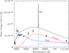 |
Fig. C.1. SED of A0620-00 simulated with our toy model, using the physical parameters of Cantrell et al. (2010). The accretion disc contribution to the SED (blue) consists of a multicolour blackbody (dashed magenta) plus an inner hot-spot with Th = 10000 K (dashed cyan). The flux of the Hα line (green Gaussian) has been scaled so that EW = 58 Å. For comparison, we overlay SED photometric points from Froning et al. (2011). |
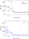 |
Fig. C.2. Simulated EWs as a function of orbital period for BH XRTs (top panel) and CVs (bottom panel). In the latter case we add the contribution of a white dwarf with TWD = 15000 K and rWD = 0.01 R⊙ to the continuum. Also, the Porb − q dependence, derived in C18, is applied. Three different inclinations are represented. |
For comparison, we also simulate the evolution of the EW for the case of CVs (bottom panel in Fig. C.2). CVs have less extreme mass ratios, with typical values ranging between q ≃ 0.1 − 1 and a mean at q ≃ 0.6 (Ritter & Kolb 2003). Since mass ratio is known to increase with Porb we apply here the relation derived in C18, i.e. q = 0.73 − 11.55 × exp[−(Porb+0.39)/0.15]. We also include an additional blackbody to account for the white dwarf emission, with fiducial parameters TWD = 15000 K and rWD = 0.01 R⊙ (Savoury et al. 2011). The figure shows that EWs are systematically lower in CVs than in BH XRTs, a natural consequence of their larger q values, which increase the relative contribution of the companion to the total flux. Only below the period gap Porb ≤ 0.085 d, CV mass ratios begin to compare to those in BH XRTs, but then the contribution of the white dwarf continuum becomes important, capping the observed EWs. In summary, our simulation predicts that the combined effect of large mass ratios and dilution by the white dwarf continuum (most important at very short Porb), leads to smaller EWs for CVs than for BH XRTs.
All Tables
Donor star densities in BH LMXBs (marked in bold), compared to those of MS and Giants with same spectral type.
All Figures
|
Fig. 1. Distribution of BH XRTs (black circles) and CVs (triangles) in the FWHM-Porb plane. Open triangles indicate eclipsing CVs, while filled triangles non-eclipsing CVs. Red triangles represent 43 CVs from C15 and blue or cyan, green, and yellow triangles the 305 SDSS CVs of dwarf novae, magnetic, and nova-like types, respectively (Inight et al. 2023). For reference, we indicate the maximum FWHM for a Chandrasekhar-mass white dwarf viewed edge-on, and the lower limit of the FWHM for accretion disc eclipses of a typical 0.82 M⊙ CV white dwarf (dotted line). We also plot the maximum FWHM of a 2.3 M⊙ neutron star viewed edge-on. The expected track of a canonical 7.8 M⊙ BH seen at 60° inclination is represented by the dashed line. |
| In the text | |
|
Fig. 2. EW versus Porb for the same sample of BHs and CVs as in Fig. 1. For reference we plot BH EW lines of constant inclination (i = 33°, 60° and 80°), computed with our toy model simulation (see Appendix C for details). The blue histogram indicates the mean EW for CVs in ten period bins. |
| In the text | |
|
Fig. 3. Power-law fits to the orbital dependence of the FWHM and EW in quiescent BH XRTs. The EW of XTE J1650-400 (open circle) has been masked from the fit. |
| In the text | |
|
Fig. 4. Diagram showing the distribution of BHs and CVs in the FWHM-Pr plane. The same symbol code is used as in Figs. 1 and 2. Vertical dots mark the BH clustering line, while the thick solid lines delineate the optimal region for separating BHs from CVs. |
| In the text | |
|
Fig. 5. Distribution of BHs and CVs in the FWHM-EW plane. The BH clustering line at FWHM = 26 × EW is indicated by dots, while the solid line marks our Fig. 4 cuts for optimal BH selection. |
| In the text | |
|
Fig. A.1. Orbital variation of FWHM and EW in XTE J1118+480 on the nights of February 7 and April 24 2011. |
| In the text | |
|
Fig. A.2. Orbital variability of FWHM (upper panel) and EW (lower panel) for 24 epochs of 10 BH XRTs with ≥50% orbital coverage. Open circles mark the three epochs with S/N≲3 spectra and thus dominated by statistical noise. The dashed blue lines show linear fits to the data. |
| In the text | |
|
Fig. A.3. Long-term (secular) variation of FWHM and EW in a sample of quiescent BH XRTs. The plot covers a period of 30 years. Every point represents an orbital average over a single epoch. The color code is as follows: blue (V404 Cyg), cyan (GRO J0422+32), magenta (N. Mus 91), red (XTE J1859+226), black (XTE J1118+480) and green (SWIFT J1357.2-0933). |
| In the text | |
|
Fig. B.1. Observed Teff vs orbital period (Porb) for donor stars in BH XRTs. Asterisks indicate ≈2 − 5 M⊙ donor stars (IMXBs) while solid black circles low-mass ≲1.5 M⊙ donors (LMXBs). The open circles mark the position of the early G-type donor in BW Cir and the nuclear-evolved companion in XTE J1118+480. Solid triangles in cyan indicate donor stars in CVs from the compilation of Knigge (2006). The blue open triangles indicate the three nuclear-evolved donors in EI Psc, QZ Ser and SDSS 1702+3229. The red line shows our empirical fit to the group of CVs and BH LMXBs, excluding BW Cir and the nuclear-evolved companions in XTE J1118+480 and the three CVs. For comparison, we also plot Teff tracks of main sequence (MS), terminal age main sequence (TAMS) and stripped-giant stars that would fill the Roche lobes for a given Porb. |
| In the text | |
|
Fig. C.1. SED of A0620-00 simulated with our toy model, using the physical parameters of Cantrell et al. (2010). The accretion disc contribution to the SED (blue) consists of a multicolour blackbody (dashed magenta) plus an inner hot-spot with Th = 10000 K (dashed cyan). The flux of the Hα line (green Gaussian) has been scaled so that EW = 58 Å. For comparison, we overlay SED photometric points from Froning et al. (2011). |
| In the text | |
|
Fig. C.2. Simulated EWs as a function of orbital period for BH XRTs (top panel) and CVs (bottom panel). In the latter case we add the contribution of a white dwarf with TWD = 15000 K and rWD = 0.01 R⊙ to the continuum. Also, the Porb − q dependence, derived in C18, is applied. Three different inclinations are represented. |
| In the text | |
Current usage metrics show cumulative count of Article Views (full-text article views including HTML views, PDF and ePub downloads, according to the available data) and Abstracts Views on Vision4Press platform.
Data correspond to usage on the plateform after 2015. The current usage metrics is available 48-96 hours after online publication and is updated daily on week days.
Initial download of the metrics may take a while.