| Issue |
A&A
Volume 699, July 2025
|
|
|---|---|---|
| Article Number | A229 | |
| Number of page(s) | 11 | |
| Section | Extragalactic astronomy | |
| DOI | https://doi.org/10.1051/0004-6361/202555268 | |
| Published online | 07 July 2025 | |
Revealing the intricacies of radio galaxies and filaments in the merging galaxy cluster Abell 2255
I. Insights from deep LOFAR-VLBI sub-arcsecond resolution images
1
Dipartimento di Fisica e Astronomia, Università di Bologna, Via Gobetti 93/2, I-40129 Bologna, Italy
2
INAF – Istituto di Radioastronomia di Bologna, Via Gobetti 101, I-40129 Bologna, Italy
3
Leiden Observatory, Leiden University, PO Box 9513, 2300 RA Leiden, The Netherlands
4
ASTRON, The Netherlands Institute for Radio Astronomy, Postbus 2, 7990 AA Dwingeloo, The Netherlands
5
Minnesota Institute for Astrophysics, University of Minnesota, 116 Church St. SE, Minneapolis, MN 55455, USA
6
Center for Astrophysics | Harvard & Smithsonian, 60 Garden St., Cambridge, MA 02138, USA
⋆ Corresponding author: This email address is being protected from spambots. You need JavaScript enabled to view it.
Received:
23
April
2025
Accepted:
16
May
2025
Abstract
Context. The high sensitivity of modern interferometers has revealed a plethora of filaments surrounding radio galaxies, especially in galaxy cluster environments. The morphology and spectral characteristics of these thin structures require the combination of high-resolution and low frequency observations, best obtained using LOw Frequency ARray (LOFAR) international stations.
Aims. In this paper, we aim to detect and characterize non-thermal filaments observed close or within the radio galaxies in Abell 2255 using deep LOFAR-VLBI observations at 144 MHz. These structures can be used to disentangle plausible scenarios describing the origin of the non-thermal filaments and connection to the motion of the host galaxy within the dense and turbulent intracluster medium (ICM), as well as the subsequent interactions between the ICM and radio jets.
Methods. Combining multiple observations, we produced the deepest images ever obtained with LOFAR-VLBI targeting a galaxy cluster, using 56 hours of observations, reaching a resolution of 0.3 − 0.5″. We detailed throughout the paper the calibration and imaging strategy for the different targets, as well as the multitude of morphological features discovered.
Results. Thanks to the high-sensitivity of LOFAR-VLBI, we revealed an unprecedented level of detail for the main cluster radio galaxies, recovering in most cases their more extended structure as well, which can only be observed at such low frequencies. In particular, we focused on the Original Tailed Radio Galaxy (Original TRG) where we distinguished many filaments constituting its tail with varying lengths (80 − 110 kpc) and widths (3 − 10 kpc). The final radio images showcase the potential of deep, high-resolution observations for galaxy clusters. With such approach, we enabled the study of hese thin, elongated radio filaments. Following their discovery, these filaments now require spectral studies to determine their formation mechanisms.
Key words: radiation mechanisms: non-thermal / techniques: high angular resolution / galaxies: clusters: individual: Abell 2255 / radio continuum: galaxies
© The Authors 2025
 Open Access article, published by EDP Sciences, under the terms of the Creative Commons Attribution License (https://creativecommons.org/licenses/by/4.0), which permits unrestricted use, distribution, and reproduction in any medium, provided the original work is properly cited.
This article is published in open access under the Subscribe to Open model. This email address is being protected from spambots. You need JavaScript enabled to view it. to support open access publication.
1. Introduction
In galaxy clusters (GCs), radio galaxies interact with the dense ambient intracluster medium (ICM), which typically leads them to exhibit distorted radio morphologies. The synchrotron emitting jets ejected from the host galaxy can be bent by ram pressure effects, while buoyancy effects can cause them to move toward the edge of the cluster. Based on the bending angle of the two jets, the radio morphology varies from wide-angle tails (WAT) to narrow-angle tails (NAT) to head-tails (HT), where the jets are bent in a common direction following the wake of the host galaxy with the latter representing the head (Miley 1980; Hardcastle & Croston 2020). High-sensitivity observations, especially with modern interferometers, are revealing the presence of a wealth of filaments both in the tail and in the surroundings of radio galaxies, particularly for the ones residing in a cluster or group environment (e.g., Hardcastle et al. 2019; Lal 2020; Ramatsoku et al. 2020; Brienza et al. 2021; Condon et al. 2021; Rudnick et al. 2022; Candini et al. 2023; Koribalski et al. 2024). Simulations show that extended bundles of magnetic field, which would be observed as filaments, are ubiquitous in turbulent magnetohydrodynamical (MHD) flows where their lengths reflect the local driving scales of the turbulence (Porter et al. 2015). Filamentary structures present new opportunities for studying the physical processes in the ICM, including their magnetic structures and the propagation of cosmic rays. They can serve as probes of shear motions, revealing the driving and dissipation scales of dynamic structures as the cluster evolves, and their widths can also provide information about the resistivity scales in the plasma. Filaments can determine an alternative site for cosmic-ray acceleration in clusters: in fact, according to Bell et al. (2019), repeated encounters with weak shocks in magnetic flux tubes in the backflows of radio galaxies could accelerate electrons to extremely high energies. Ultimately, the seed electrons upon which the re-acceleration operates on cluster-scales likely come from current or past active galactic nuclei (AGN) activity: given that particle acceleration via shocks and turbulence is an inefficient process (for a complete review see Brunetti & Jones 2014), these seed electrons are thought to be essential for the formation of diffuse emission in the form of radio halos and relics (Vazza & Botteon 2024). Thus, beyond simple ram-pressure deflection, we must explore a wider range of the mutual interactions between ICM and radio galaxies to unveil the physical mechanisms responsible for the complex morphology of these objects (Rudnick et al. 2022). Observing distorted filaments and substructure of nearby radio galaxies offers a unique opportunity to explore the nature and origin of these features; in particular, the re-energization processes and the role of internal and external magnetic fields. From the literature, these features are known to have steep radio spectra (α > 1.31), with signs of steepening along the filament lengths and widths (Rudnick et al. 2022; Brienza et al. 2025), projected lengths ranging between 10 s and 100 s kpc, and widths from a few kpc down to 350 − 500 pc (as observed in Perseus cluster, van Weeren et al. 2024). These characteristics underline the necessity of sensitive, low-frequency and high-resolution observations to detect and disentangle such filaments.
The International LOw Frequency ARray (LOFAR) Telescope (ILT, van Haarlem et al. 2013) represents an excellent candidate for this scope. Having baselines extending to almost 2000 km, this interferometer provides a unique resolution down to 0.3″ at the high-band antenna (HBA) frequencies of 144 MHz (Morabito et al. 2022), making it ideal for targeting filaments in tails of radio galaxies and within the ICM. Recently, the calibration and imaging procedure has been standardized with the development of a LOFAR Very Long Baseline Interferometry (VLBI) pipeline (Morabito et al. 2022), capable of calibrating HBA data using full ILT array and imaging single target sources down to sub-arcsecond resolution at 144 MHz. This pipeline was recently upgraded to a new version which implements the Common Workflow Language (CWL) and which has become the new standard for LOFAR-VLBI data2 (van der Wild, in prep.). In the past years, this pipeline has been successfully used for targeting galaxy clusters and groups (e.g., Timmerman et al. 2022; Cordun et al. 2023; Timmerman et al. 2024; Ubertosi et al. 2024; van Weeren et al. 2024; Pasini et al. 2025).
In this paper, we use the ILT to observe the radio galaxies and filaments in the galaxy cluster Abell 2255 (hereafter A2255) at sub-arcsecond resolution. This is a merging galaxy cluster (z = 0.0806) exhibiting morphologically complex radio structures on multiple scales (see Botteon et al. 2020, 2022, and references therein for a more detailed description). Several optical and infrared studies reported a total number of confirmed member galaxies that range from 300 to 500 (depending on the radius selection criteria), using both spectroscopic and photometric techniques (Yuan et al. 2003; Shim et al. 2011; Tyler et al. 2014; Golovich et al. 2019). Miller & Owen (2003) focused in particular on the fraction of AGN. Using Karl G. Jansky Very Large Array (VLA) data at 1.4 GHz, they found that A2255 has an abnormal abundance of radio galaxies compared to other clusters, which is possibly motivated by the cluster’s dynamical state, even if this is not yet clear from optical observations (Burns et al. 1995; Yuan et al. 2003). Radio galaxies in A2255 have been widely observed in the past (e.g., Harris et al. 1980; Burns et al. 1995; Miller & Owen 2003; Govoni et al. 2006; Pizzo & de Bruyn 2009; Pizzo et al. 2011; Terni de Gregory et al. 2017; Botteon et al. 2020, 2022). Four tailed radio galaxies reside in the cluster: following the nomenclature introduced by Harris et al. (1980), there are three NAT sources, namely: the Original Tailed Radio Galaxy (Original TRG), the Goldfish, and the Beaver, along with a WAT known as the Embryo. Together with these, there is also a Fanaroff-Riley II (FRII, Fanaroff & Riley 1974) radio galaxy located, in projection, close to the cluster center called the Double. Observations for these sources were performed by Govoni et al. (2006) at high frequencies, using VLA in C- and X-band providing resolution of 2″; they also studied the fractional polarization of these sources, finding mean values around 14% for the NATs. The Goldfish has been observed also with VLA at 15 GHz, reaching an angular resolution of 0.47″ × 0.44″ (Terni de Gregory et al. 2017) and revealing strong projection effects impacting its morphology. Together with observations of cluster radio galaxies, Govoni et al. (2005) discovered the presence of strongly polarized filaments (20 − 40% of fractional polarization) in the cluster radio halo at 1.4 GHz, with a rectangular shape and regions of ordered magnetic field of ∼400 kpc in size. They were reported also subsequently using the Westerbork Synthesis Radio Telescope (WSRT) by Pizzo & de Bruyn (2009) and Pizzo et al. (2011). Recently, thanks to deep LOFAR observations (75 hours at 145 MHz, with rms noise of 43 μJy beam−1, resolution of 4.7″ × 3.5″, as shown in Fig. 1; 72 hours at 49 MHz, rms noise of 730 μJy beam−1, resolution of 11.5″ × 8.2″), Botteon et al. (2020, 2022) detected the presence of additional filamentary and distorted structures on different scales with a very steep spectrum (α > 2) embedded in the radio halo, whose association with optical counterparts of the cluster radio galaxies is not trivial, considering also that these filaments are detectable only at LOFAR frequencies.
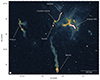 |
Fig. 1. Zoom-in on Abell 2255’s center at 145 MHz, resolution of 4.7″ × 3.5″, adapted from Botteon et al. (2022). The main cluster member radio galaxies that are the focus of this paper are highlighted in white and labeled the same as in Harris et al. (1980) and Botteon et al. (2020). The restoring beam size is shown in the bottom-left corner. |
In this work, we aim to observe the tails and filaments that populate the cluster environment using the high-resolution, low-frequencies capabilities of the ILT. We produced radio maps at 144 MHz at sub-arcsecond resolution, targeting the brightest cluster member radio galaxies: using 56 hours of observations, this makes the deepest LOFAR-VLBI images ever targeting a galaxy cluster. Thanks to the high-resolution and sensitivity of LOFAR-VLBI we detected, for the first time, a multitude of substructures related to these radio galaxies; they are mostly filamentary and observable only at such low frequencies. Particular attention was given to the Original TRG, which revealed the presence of filaments related to its tail extending for almost 300 kpc presuming a complex origin scenario involving the turbulent environment which surrounds it. In this paper, we focus on the methodology used to produce the deep LOFAR-VLBI images and on a morphological study of the Original TRG. In an upcoming paper, this analysis will be combined with high-resolution spectral index maps resulting from the combination of LOFAR-VLBI data with upgraded Giant Metrewave Radio Telescope (uGMRT) and the VLA at higher frequencies.
In this paper, we assume a flat ΛCDM cosmology, with H0 = 70 km s−1 Mpc−1, Ωm = 0.3, and ΩΛ = 0.7. At the redshift of Abell 2255, 1″ corresponds to a linear scale of 1.512 kpc.
2. Data calibration and imaging
A2255 was first observed for 72 hours by LOFAR in the period June to November 2019 (project LC12_017, P.I. R.J. van Weeren). The cluster is located at about 5° from the Euclid Deep Field North (EDFN), which made it possible to observe the two targets simultaneously using two different LOFAR beams (Bondi et al. 2024). After these first observations, A2255 was again observed for an additional 226 hours as the secondary target during the very deep EDFN observations carried out in the period 2022–2023 (project LT16_005, P.I. P.N Best). For this paper, we selected only observations coming from the first set of 72 hours, because the latest ones are still in the phase of processing. The 72 hours were split in 9 runs and each 8 hour observation was calibrated individually.
After describing the preliminary steps involved in the calibration of the Dutch stations, for both direction-independent (DIE) and direction-dependent (DDE) effects, we detail the procedures on the international stations (IS): for their calibration strategy, we followed the procedures extensively described in Morabito et al. (2022), with different tailored adjustments, especially in the imaging step, required by the high-complexity radio morphology of the field containing A2255, with the combination of extended and structured radio galaxies overlapping the cluster radio halo.
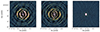 |
Fig. 2. Self-calibration results on the delay calibrator 4C +64.21 for one observing run. From left to right: Self-calibration cycle 0 (sole imaging), cycle 1 (only scalarphasediff and scalarphase solutions), cycle 19 (final image, solving also for scalarcomplexgain). |
List of the LOFAR observations used in this paper.
2.1. Initial calibration of the Dutch stations
The first step provides calibration of the visibilities following the standard procedure used for the LOFAR Two-metre Sky Survey (LoTSS, Shimwell et al. 2017, 2019, 2022). After downloading data from the LOFAR Long-Term Archive (LTA), both for primary calibrator and target, for each observation, we used Prefactor (de Gasperin et al. 2019) solutions from Botteon et al. (2020, 2022) on the primary calibrator, which was 3C48 for all the observations. This pipeline corrects for the polarization alignment, clock delays between stations, and bandpass, for both Dutch and international stations. Prefactor is used also for the target field (A2255) to correct for DIE on the Dutch stations. After applying the solutions found for the primary calibrator to the target, it calibrates the phases against a sky model from the TIFR GMRT Sky Survey (TGSS, Intema et al. 2017).
We then further processed our data to correct for DDE using ddf-pipeline (Shimwell et al. 2017; Tasse et al. 2021), which uses killMS (Tasse 2014; Smirnov & Tasse 2015) for direction-dependent calibration and DDFacet (Tasse et al. 2018) to apply direction-dependent solutions during imaging. The output image of the target field at 6″ resolution, corrected for both DIE and DDE on the Dutch stations, has been used to assess the quality of the observation.
2.2. Calibration of the International stations
Once the Dutch array was fully calibrated, we proceeded with the calibration of the IS. Following the strategy described in Morabito et al. (2022), solutions from the Dutch array corrected for both DIE and DDE were transferred to the original measurement sets including also the IS. Then, after checking the contribution of bright, off-axis sources (so-called A-team sources, that were sufficiently far to avoid contaminating the target field), the datasets were concatenated into sub-bands of 1.95 MHz each. These sub-bands were phase-shifted toward the direction of an in-field calibrator for the calibration of the IS, required for correcting direction-independent dispersive delays, and concatenated in frequency into a single measurement set.
For our field, we searched for the best available in-field calibrator using the Long Baseline Calibrator Survey (LBCS, Jackson et al. 2016, 2022). The selected source was 4C +64.21 (RA: 17h19m59s, Dec: 64 ° 04′37″, Pilkington & Scott 1965), a powerful radio source, compact on arcsec-scale, with flux density of ∼4.87 Jy at 144 MHz. Given that it shows the presence of two components at 0.3″ resolution (and was observed at multiple frequencies throughout the radio spectrum), we built a sky model distributing the flux density among two Gaussian components, with the same flux ratio as the one in the full resolution map. To better reproduce the spectral index for the calibrator, we used flux density measures at multiple radio frequencies, following de Jong et al. (2024): in particular, the 8C survey at 38 MHz (Hales et al. 1995), the VLA Low-frequency Sky Survey at 74 MHz (VLSS, Cohen et al. 2007), the 6C survey at 151 MHz (Hales et al. 1990), the Westerbork Northern Sky Survey at 325 MHz (WENSS, Rengelink et al. 1997), the Texas Survey at 365 MHz (Douglas et al. 1996), and the NRAO VLA Sky Survey (NVSS, Condon et al. 1998) at 1.4 GHz. With flux densities and frequencies we fitted a second-order logarithmic polynomial
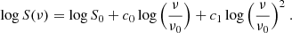 (1)
(1)
Using ν0 = 144 MHz as the reference frequency, we ended up with c0 = −0.013 and c1 = −0.90. These parameters, together with the position of the Gaussian subcomponents, made the initial sky model that we used for the in-field calibrator.
List of the target sources with the final map properties.
We used facetselfcal (van Weeren et al. 2021), which uses the Default Preprocessing Pipeline (DP3, van Diepen et al. 2018; Dijkema et al. 2023) and WSClean (Offringa et al. 2014; Offringa & Smirnov 2017) to perform self-calibration. It allows us to correct phases and amplitudes, thereby minimizing the differences between the data and the sky model, namely by updating the latter in each self-calibration cycle. We followed the procedure adopted by de Jong et al. (2024) with some minor adjustments. In particular, during the self-calibration cycles, we solved for:
-
scalarphasediff: solution interval 128 s, frequency smoothness 4.0 MHz;
-
scalarphase: 32 s, frequency smoothness 1.0 MHz;
-
scalarcomplexgain: 53 min, frequency smoothness 4.0 MHz, one solution each 10 channels.
We ignored all the baselines shorter than 40 000λ, corresponding to an angular scale of about 5″ at 144 MHz, using the parameter --uvmin, to prevent possible incompleteness in the sky model. We phased up LOFAR’s core stations to form a large, virtual, narrow field of view (FoV) station, to reduce the interference from unrelated nearby radio sources especially at short baselines. Through facetselfcal, we also averaged the input data down to 32 s in time and 488 kHz in frequency and used a Briggs weighting with robustness of −1.5 for the imaging (Briggs 1995). At the end of the self-calibration routine on the in-field calibrator, one hierarchical data format 5 (h5parm) solution file was produced for each calibration step and one containing all the solutions merged, with phases and amplitudes corrections. We performed 20 self-calibration cycles providing the best solutions for visibilities (Fig. 2). Among the 9 available observations, two (namely L728074 and L746864) have been discarded because of the significantly higher image noise once including the IS (between 30 − 40% with respect to the other runs). We ended up with 7 runs (meaning 56 hours of observing time on target), that have been used for the long baselines calibration and imaging. The main characteristics of the selected observations are listed in Table 1
2.3. Self-calibration on target cluster radio galaxies
With the IS fully calibrated, we imaged the main cluster radio galaxies with LOFAR-VLBI at 144 MHz at sub-arcsecond resolution. For each of the 7 runs, the concatenated datasets produced by the LOFAR-VLBI pipeline were phase-shifted toward 5 targets and averaged. The selected targets correspond to the main cluster radio galaxies: the Double, the Original TRG, the Goldfish, and the Beaver. First, we applied the h5parm, DIE calibration solutions from the in-field calibrator to all the sources for each observation individually. Given the large distance of the in-field calibrator from the pointing center (0.8°) and the complex morphology of the targets, we used compact and bright sources closer to the cluster as additional calibrators to improve the calibration solutions on targets in a similar way to the faceting (van Weeren et al. 2016) or the wide-field direction-dependent calibration (de Jong et al. 2024). The radio source J171259+640931 was used as additional calibrator for the Double and the Goldfish. After performing the self-calibration, solving for scalarphase and scalarcomplexgain, and phasing-up the core stations, to reduce the FoV and so the effects from the nearby radio emission from the cluster center, we transferred the calibration solutions to the two targets and proceeded with self-calibration. For the Double, we solved for tec, scalarphase, and scalarcomplexgain, avoiding all the baselines below 10 000λ (corresponding to ∼20″) and phased-up the core stations. For the Goldfish, we solved for tecandphase and scalarcomplexgain and phased-up the superterp stations, avoiding all the baselines below 5000λ (corresponding to ∼41″). The Double was also used as additional calibrator for the Original TRG: for the main tailed cluster radio galaxy, we solved for tec, scalarphase, and scalarcomplexgain, avoiding all the baselines below 10 000λ and phased-up the core stations. Including shorter baselines for these extended sources, with respect to what was done for the in-field calibrator, was required to add more large-scale signal during calibration. For Beaver and the Embryo instead, we used the radio source J171423+635707 as an additional calibrator. Given the dominant low surface brightness extended emission in these sources, self-calibration did not result in any improvement in the image quality: for this reason, we simply applied the solutions from J171423+635707 and imaged the two targets. After self-calibration (where possible), we imaged each source with WSClean using wgridder (Arras et al. 2021; Ye et al. 2022), combining all the calibrated MS at once, using automatic masking and multiscale deconvolution (Offringa & Smirnov 2017) to better deal with their extended structure.
3. Morphological analysis of cluster member radio galaxies
In this section, we present the final imaging results for the target radio galaxies, as well as their morphological detailing. Their main properties are listed in Table 2.
3.1. The Double
The Double, also known as J171329+640249 (Miller & Owen 2002), is a FRII radio galaxy located, in projection, at about 600 kpc from the cluster center. It exhibits a double-lobed morphology with a total extent of almost 50 kpc (≈35″). Our new LOFAR-VLBI sub-arcsecond resolution image of the source is shown in Fig. 3. We resolve the core and the two jets departing from it up to the hotspots. Both lobes show edge-brightening at their tips, possibly resulting from the shocks formed by the interaction with the ICM, and extend for about 21 kpc (north) and 23 kpc (south), measured above the 3σrms. At this detection level, the source has a flux density of 0.95 ± 0.10 Jy at 144 MHz. Assuming a spectral index α = 0.65 (Botteon et al. 2020), the source has a rest-frame luminosity L144 ∼ 1.48 × 1025 W Hz−1: the classical FRI-II luminosity break is around L150 ∼ 1026 W Hz−1 (Fanaroff & Riley 1974; Ledlow & Owen 1996), so the Double can be classified as “FRII-Low” (Mingo et al. 2019). The southern hotspot is shifted with respect to the initial direction of the jet, which ends up into another bright spot in the same lobe: this may suggest the presence of multiple hotspots (Hardcastle et al. 1997). In the southern hotspot there is also a narrow arc-like structure (labeled in Fig. 3) which, as for other similar objects, could represent a well-collimated backflow (Leahy et al. 1997). The northern hotspot is instead surrounded by a ring-shaped radio brightness enhancement (labeled in Fig. 3). These rings are unusual, but not unique: they were already observed in other radio galaxies, for instance, in the western hotspot of Hercules A (Dreher & Feigelson 1984; Timmerman et al. 2022), in 3C 310 (Morrison & Sadun 1996), or in 3C 219 (Perley et al. 1980). Several scenarios can explain the formation of the rings (Saxton et al. 2002; Gizani & Leahy 2003), involving mainly the shocks and the inner lobes model. In the former, the rings are shocks with circular geometry, caused by backflows in the cocoon, which introduce adiabatic compression and particle acceleration. In the latter, instead, rings arise from material deposited by new jets in the lobe and separated from it by a contact discontinuity. From the sole radio map, disentangling the correct one is non-trivial. The presence of rim-brightening, observed in the ring around the northern hotspot in the Double, favors the shock model because it is the only one that can explain such feature, as also shown in simulations (Meenakshi et al. 2023). Additional information, such as the spectral index, is still required to reliably discriminate between the proposed models or (if necessary) to motivate new ones. Further investigation of all these aspects is beyond the scope of this paper.
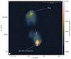 |
Fig. 3. The Double at 144 MHz; resolution 0.30″ × 0.24″, rms noise 18 μJy beam−1. This image was obtained using Briggs weighting, robust = −0.5, and multiscale. The restoring beam size is shown in the bottom-left corner. The red cross identifies the optical position of the host galaxy as listed in Table 2. |
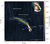 |
Fig. 4. The Original Tailed Radio Galaxy (Original TRG) at 144 MHz; resolution of 0.34″ × 0.24″, rms noise of 18 μJy beam−1. This image was obtained using Briggs weighting, robust = −0.5, and multiscale. The restoring beam size is shown in the bottom-left corner. Top-right corner: Zoom-in (22 kpc) on a region close to the host galaxy, whose optical position (listed in Table 2) is identified with a red cross. |
3.2. The Original TRG
The Original TRG, also known as 7C 1712+6406 (Hales et al. 2007), is a NAT radio galaxy, classified as a FRI by Capetti et al. (2017). Previous studies at higher frequencies (VLA L-, C-, and X-band; Govoni et al. 2005, 2006) reported a source extension of about 2.5′ with a mean fractional polarization up to 14%. Our deep, high-resolution map provided by LOFAR-VLBI is presented in Fig. 4. We reveal several new substructures along the tail, which otherwise would have been considered as a unique, continuous component. First, we precisely identified the host galaxy (red cross in Fig. 4) and the ejection location of the two relativistic jets. Following the tail extension in the north-east direction, we observed three turbulent eddies at distances between 10 and 30 kpc from the host galaxy, evenly spaced from each other (∼9 kpc). We note that they possibly arise from the instabilities developed in the downstream of the radio galaxy. Interestingly, the entire tail seems to depart only from the northern jet: the southern one, instead, seems to interrupt abruptly, as also observed at higher frequencies by Govoni et al. (2006). Thanks to the combination of high-sensitivity and resolution we also detect, for the first time, multiple filamentary structures that constitute the tail of the radio galaxy. At 144 MHz we reveal the presence of an extended filament at the lower bound of the main tail, labeled F1 and which follows its shape, just after an emission gap of around 10 kpc from the southern jet termination. This may suggest that some event could have prevented the development of a tail from the southern jet for a fixed amount of time during the host galaxy motion. However, the lack of the southern tail can also result from projection effects, where it can be bent and hidden behind the northern one. The southern jet is connected to a bright emission patch, having flux a density of ∼0.08 Jy beam−1 (at 10σrms), via two tethers similar to the ones observed in the radio galaxy IC711 in Abell 1314 (van Weeren et al. 2021) or in the MysTail in Abell 3266 (Rudnick et al. 2021). Along with F1, we detected a horizontal filament at the north-east end of the main tail and a vertical filament that departs from this last one toward the north. Between the upper end of the main tail and the west side of the horizontal filament there is another filamentary feature that emerges, labeled as F2 in Fig. 4. Despite resembling the F1 filament, it is attached directly to the horizontal filament, which would suggest a plausibly different origin and that is might be more connected to what is happening above the horizontal filament. A more quantitative description of the filaments, including their lengths and widths, is presented in Sect. 4.
The characteristics of plasma in the main tail and in the filaments cannot be determined solely on the basis of a morphological analysis, but from a spectral index analysis instead. We defer such an analysis to an upcoming paper, where we will present and discuss images of the Original TRG and its filaments obtained at 144, 1260, and 1520 MHz with a resolution of 1.5″ (De Rubeis et al., in prep.). Spectral index information between 49 and 145 MHz from Botteon et al. (2022) (12.5″ resolution) on the Original TRG reports nuclear values around α ∼ 0.5 − 0.6, with signs of spectral aging along the tail up to α ∼ 2, corresponding to what we identified as the vertical filament. The combination of low-resolution and low-frequency implies a significant contribution of the diffuse emission from the radio halo in which this radio galaxy is situated; this motivates a follow-up at higher frequency and resolution, to extract the intrinsic spectral properties of the radio galaxy.
At almost 50″ from the Original TRG there is the Sidekick radio galaxy (z = 0.071436, Miller & Owen 2003), another cluster member radio galaxy for which we resolve its double-jetted structure, which extends for ∼3.6 kpc and then ends up into a tail that goes south for around 80 kpc.
3.3. The Goldfish
The Goldfish, also known as 7C 1713+6407a (Hales et al. 2007), is a NAT radio galaxy classified as FRI. A deep LOFAR image made with the Dutch array (Fig. 1) revealed an extended head and a narrow tail of ∼300 kpc length that ends up mixing with a diffuse feature, known as Counter-comma (Botteon et al. 2020), whose origin is still unclear. High-resolution, high-frequency observations (in the L-, C-, and Ku-band) resolved the head of the radio galaxy, with two jets that depart from the core with a gap of 1.5″ observed for both of them (Owen & Ledlow 1997; Terni de Gregory et al. 2017). From a deep LOFAR-VLBI map (presented in Fig. 5), we resolved the core and the region immediately close to the head (within 50 kpc from the host), where the ram pressure effects on the jets can be observed; this is the case, in particular, for the northern one, which is deflected by almost 90° as soon as it leaves the core region. At sub-arcsecond resolution, we also detect the tail emission up to the connection with the Counter-comma, with the presence of a region of increased surface brightness at around 170 kpc from the core. Interestingly, the tail presents a helical morphology right after the head region, as if the two jets are spiraling around each other before linking back into a single tail that then extends southwards. This wobbling, similar to what happens for the Beaver radio galaxy (Sect. 3.4, but on smaller scales), can be due to different reasons related to the motion of the host galaxy or the instabilities developed behind it.
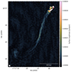 |
Fig. 5. The Goldfish at 144 MHz; resolution of 0.55″ × 0.41″, rms noise of 29 μJy beam−1. This image was obtained using Briggs weighting, robust = −0.5, and multiscale. The restoring beam size is shown in the bottom-left corner. The red cross identifies the optical position of the host galaxy as listed in Table 2. |
3.4. The Beaver
The Beaver, also known as 7C 1712+6352 (Hales et al. 2007), is a NAT radio galaxy placed at ∼1.5 Mpc from the cluster center. Low-frequency observations made with LOFAR Dutch array at 144 MHz have revealed a twisted tail that extends for more than 1 Mpc, before fading into the cluster radio halo (Fig. 1). Deep LOFAR-VLBI map is shown in Fig. 6 (left panel). At sub-arcsecond resolution, we mainly resolved the core region and the two jets departing from it and also the first, brighter part of the tail up to the point at which the two jets get close for the first time along the tail, before developing its characteristic corkscrew feature (fully depicted in Fig. 1). The rest of the tail was not detected because of the lower surface brightness and the time and bandwidth smearing effects, reducing the intensity far from the pointing center (Bridle et al. 1999).
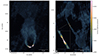 |
Fig. 6. Left: the Beaver at 144 MHz, resolution of 0.54″ × 0.40″, rms noise of 27 μJy beam−1. The image was obtained using Briggs weighting, robust = − 0.5, and multiscale. Right: Embryo at 144 MHz, resolution of 0.55″ × 0.40″, rms noise of 40 μJy beam−1. The image was obtained using Briggs weighting, robust = 0.5, and multiscale. Bottom-left panel: zoom-in view of approximately 32 kpc centered on the source. For both images, the restoring beam size is shown in the bottom-left corner. |
3.5. Embryo
The Embryo, also known as GB6 B1714+6405 (Gregory et al. 1996, z = 0.08001), is a WAT radio galaxy located, in projection, at about 1.5 Mpc from the cluster center. Its radio emission at 144 MHz extends for ∼600 kpc, considering the more diffuse emission generated by ram pressure effects in correspondence of the lobes. The deep, sub-arcsecond resolution map is shown in Fig. 6 (right panel). As for the Beaver, we resolve the core region with the inner jets; the southern jet is brighter than the northern one by a factor of 2, considering the 5σrms emission within a projected distance of 10.5 kpc from the core. Moreover, there are multiple bright spots along the northern jet, possibly hinting at the central black hole’s duty cycle. The jets are maintained collimated (3.5 − 6 kpc) before experiencing the effects of the ICM and becoming bent. Following Laing et al. (1999) (Eq. (1)) and assuming isotropic emission in the source rest-frame and a spectral index α = 0.5 (from Botteon et al. 2020), we can constrain the angle to the line of sight to be θ ≤ 60° and the jet velocity to be ≥0.5c. The morphology of the Embryo suggests possible hints for the kinematics of the host galaxy within the ICM: the slight bending of the northern jet can be caused by the motion of the host galaxy toward the north-east direction, with the southern jet which is not affected by such dynamics.
4. Characterization of the filaments in the Original TRG
In this section, we describe and discuss the properties related to the morphology and the emissivity of the filaments detected in the Original TRG, based on what we have observed at 144 MHz from LOFAR-VLBI. We distinguished several morphological features presented in Sect. 3.2 and highlighted in Fig. 4. Projected lengths can be directly measured from the map. The main tail, which develops from the northern jet, extends for ∼140 kpc before linking with the horizontal filament. The horizontal filament extends for about 110 kpc on the east-west direction, with a forking on the west side. The vertical filament’s length is ∼105 kpc. The F1 filament has length of ∼83 kpc, measured from the gap to the horizontal filaments (where it ends up); F2 is instead more challenging to isolate with respect to the other features, given the tight connection with the horizontal filament and the upper end of the main tail. In this case, spectral index information will be helpful in determining the properties of its electron population and, thus, its origin. Overall, considering all three components (main tail, horizontal and vertical filament) the Original TRG complex extends for at least ∼3′ (∼270 kpc).
To measure the width of the filaments and the main tail, we traced multiple transversal cuts (as the one shown in Fig. 7, dashed white arrow) across the Original TRG, obtaining a spatial surface brightness profile for each cut. The rms noise of the image was quadrature-subtracted to the brightness values and the resulting profiles were fitted with single or multiple Gaussian profiles. For the fit, we used the non-linear least squares method. The number of Gaussians of the model function was chosen by a visual inspection of the surface brightness profiles along the cuts. The amplitude, standard deviation, and center of each Gaussian were allowed to vary; as an initial guess, we used values of 1.0 for the amplitude and the standard deviation, while for the center we used equidistant values (depending on the number of Gaussians) distributed within the length of the cut. The beam-deconvolved full width at half maximum of the fitting Gaussian is then considered to be the width of the corresponding feature. An example of three-Gaussian fit for the central part of the Original TRG, which includes F1, the main tail, and F2, is shown in the bottom panel of Fig. 8. The main tail has widths that start from 1.8 kpc (at the point where it starts developing from the northern jet) to 3.5 − 4.7 kpc between the eddies. Moving upward, the width ranges between 8 and 13 kpc: then, it mixes up with the horizontal filament. The F1 filament has width ranging between 3 and 4.2 kpc (from the gap upward); F2, instead, exhibits a width of 5 kpc. The horizontal filament, when observed at such high-resolution, is resolved into multiple substructures – rather than appearing as a single monolithic structure, as highlighted in the top panel of Fig. 7. We measured its width in the central brighter part (where there is a high-enough signal-to-noise ratio), to be ∼8 − 10 kpc, even if there it is difficult to distinguish between the main tail, the horizontal filament and F2 as they are co-spatial. At the edges the detection is at the noise level. The vertical filament has almost constant width of about 4.5 kpc, with a forking at the bottom where it connects in two different parts to the horizontal one.
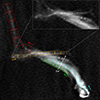 |
Fig. 7. Same LOFAR-VLBI map for the Original TRG shown as in Fig. 4 highlighting the regions used for determining the main morphological features associated to the radio galaxy using different colors. Arrow represent the direction of the transversal cut used to retrieve the filaments’ widths depicted in the bottom panel of Fig. 8. Top right corner: Details of the horizontal filament to highlight the main morphological patterns coexisting in this region. |
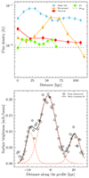 |
Fig. 8. Spatial trends along the Original TRG and its filaments from regions highlighted in Fig. 7. Top: Flux density along the main features of the Original TRG, highlighted in different colors. Error bars refer to the errors on flux densities, calculated assuming a 10% flux uncertainty (as for the LoTSS, Shimwell et al. 2022). Colored arrows indicate the direction followed by the spatial trends. Bottom: Profile across the Original TRG following the cut depicted in Fig. 7. The noise-subtracted data are shown as open circles. The black solid line shows the total fit using three-Gaussian fit. The three Gaussians (individually shown with red dashed lines) correspond (from left to right) to F1, the main tail, and F2, respectively. |
In Fig. 8 we show also the flux density profiles along the main feature highlighted for the Original TRG in Fig. 7: the main tail (in cyan), F1 (in green), the horizontal filament (in orange) and the vertical one (in red). The brightness increase in the center of the horizontal filament is due, at least in part, to the overlap with the upper end of the main tail and (apparently) the F2 filament. High-resolution spectral index studies are crucial to disentangle the different emitting components and reconstruct their origin in this part. At high angular resolution, filaments also show their non-thermal emission in multiple patches; this could indicate that their formation process does not act homogeneously along the filament’s extension and, instead, could have some local contribution that enhances the radio emission.
Having thin and long non-thermal filaments, with the horizontal and vertical ones that also show a particularly straight shape, may suggest a common formation scenario with the E-fils observed by Rudnick et al. (2022) in the radio galaxy 3C40B in Abell 194. In that case, the preferred formation scenario relied on the amplification of the magnetic field through shear stretching of magnetic field lines: the observed filaments would then be made by smaller bundles of illuminated and aligned fibers, held together by tension along the field lines. The thickness of the fibers should reflect the transverse resistivity scales, while their length reflects the driving scales of the local turbulent flow (Vazza et al. 2018). For A2255, given the presence of turbulence associated to the merging state of the cluster, this can reach the cluster scale. From the filaments’ lengths we can evaluate its dynamical lifetime, which is essentially the cascading time of the turbulent eddy on scale L. Assuming a turbulence Mach number of ℳ = 1/2 and a characteristic ICM sound speed cs ∼ 103 km/s (Porter et al. 2015), we end up with
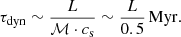 (2)
(2)
Our filaments have lengths ranging between 80 and 110 kpc, resulting in τdyn ∼ 160 − 220 Myr: this is comparable to the synchrotron radiative lifetimes (107 − 108 yr), meaning that electrons have sufficient time to emit all their energy via synchrotron radiation before the filament gets dissipated by the turbulence. Spectral index information along the filaments will enable us to constrain particle acceleration (if present) as well as the spatial diffusion coefficient required to observe radio emitting electrons on such scales. The stretching of the magnetic field lines implies magnetic field amplification by a factor proportional to ρv2/l, where ρ is the density of the turbulent ICM, with characteristic velocity, v, on the driving scale, l. This causes enhancement in the magnetic field pressure PB = B2/8π, which becomes compatible with the thermal pressure, reducing the plasma beta of the filaments βF = Pgas/PB. We expect the filaments, given also their straightness, to have very low plasma beta (approaching unity), being high-magnetic pressure regions. In support of this scenario, some cases have shown an overlap between the presence of non-thermal radio filaments and the absence of thermal, X-ray emitting ICM (Rudnick et al. 2022).
5. Conclusions
In this work, we present LOFAR-VLBI observations at sub-arcsecond resolution of the brightest cluster radio galaxies in the merging cluster Abell 2255, obtained using 56 hours of observations. These images represent the deepest ones obtained to date using LOFAR-VLBI for a galaxy cluster. The unique resolution and sensitivity capabilities of LOFAR IS revealed unprecedented structures connected to the radio galaxies, particularly with respect to the Original TRG, where several filaments have been discovered around the tail and attached to its upper end. Despite being already observed in other galaxy clusters and groups, especially in the presence of a turbulent ambient medium, this represents the first time that these objects have been observed at such high resolution, demonstrating the potential of LOFAR-VLBI observations for these elongated, non-thermal filaments. They have lengths ranging from 80 to 110 kpc, with varying widths along their extension (3 − 10 kpc), as seen for other cases observed in other clusters (such as in Abell 194, Rudnick et al. 2022). Being thin and straight, there is the possibility that, as the ones in A194, they present very low plasma beta due to the amplification of magnetic field caused by shear stretching of field lines. One peculiarity observed is the patchiness of the radio emission along the filaments, which may suggest further hints about their formation scenario. To constrain the nature and the origin of these filaments, we will present in an upcoming paper observations at higher frequencies of the Original TRG using uGMRT (Band 5) and VLA (L-band). Providing a resolution of 1.5″, these images will allow for high-resolution spectral index analyses of the filaments to constrain their radio spectral properties and disentangle multiple spectral components that are co-spatial in the Original TRG from lower-resolution studies. In addition, we will present also additional filaments detected with LOFAR-VLBI at 1.5″ resolution on larger scales extending for ∼250 kpc east of the Original TRG, originally known as the Trail (Botteon et al. 2020). VLA data will also allow polarization analysis, which has been observed in similar structures up to 40 − 50% (Rudnick et al. 2022).
We use the convention S(ν)∝ν−α for synchrotron spectrum, with α > 0
Acknowledgments
EDR and CG are supported by the Fondazione ICSC, Spoke 3 Astrophysics and Cosmos Observations. National Recovery and Resilience Plan (Piano Nazionale di Ripresa e Resilienza, PNRR) Project ID CN_00000013 “Italian Research Center for High-Performance Computing, Big Data and Quantum Computing” funded by MUR Missione 4 Componente 2 Investimento 1.4: Potenziamento strutture di ricerca e creazione di “campioni nazionali di R&S (M4C2-19)” – Next Generation EU (NGEU). MB acknowledges support from INAF under the Large Grant 2022 funding scheme (project “MeerKAT and LOFAR Team up: a Unique Radio Window on Galaxy/AGN co-Evolution”). JMGHJdJ acknowledges support from project CORTEX (NWA.1160.18.316) of research programme NWA-ORC, which is (partly) financed by the Dutch Research Council (NWO), and support from the OSCARS project, which has received funding from the European Commission’s Horizon Europe Research and Innovation programme under grant agreement No. 101129751. This manuscript is based on data obtained with the International LOFAR Telescope (ILT). LOFAR (van Haarlem et al. 2013) is the Low Frequency Array designed and constructed by ASTRON. It has observing, data processing, and data storage facilities in several countries, which are owned by various parties (each with their own funding sources), and which are collectively operated by the ILT foundation under a joint scientific policy. The ILT resources have benefited from the following recent major funding sources: CNRS-INSU, Observatoire de Paris and Université d’Orléans, France; BMBF, MIWF-NRW, MPG, Germany; Science Foundation Ireland (SFI), Department of Business, Enterprise and Innovation (DBEI), Ireland; NWO, The Netherlands; The Science and Technology Facilities Council, UK; Ministry of Science and Higher Education, Poland; The Istituto Nazionale di Astrofisica (INAF), Italy. This research made use of the LOFAR-IT computing infrastructure supported and operated by INAF, including the resources within the PLEIADI special “LOFAR” project by USC-C of INAF, and by the Physics Dept. of Turin University (under the agreement with Consorzio Interuniversitario per la Fisica Spaziale) at the C3S Supercomputing Centre, Italy. This research made use of Matplotlib (Hunter 2007), APLpy (an open-source plotting package for Python, Robitaille & Bressert 2012), Astropy (a community-developed core Python package and an ecosystem of tools and resources for astronomy, Astropy Collaboration 2022).
References
- Ahn, C. P., Alexandroff, R., Allende Prieto, C., et al. 2012, ApJS, 203, 21 [Google Scholar]
- Alam, S., Albareti, F. D., Allende Prieto, C., et al. 2015, ApJS, 219, 12 [Google Scholar]
- Arras, P., Reinecke, M., Westermann, R., & Enßlin, T. A. 2021, A&A, 646, A58 [NASA ADS] [CrossRef] [EDP Sciences] [Google Scholar]
- Astropy Collaboration (Price-Whelan, A. M., et al.) 2022, ApJ, 935, 167 [NASA ADS] [CrossRef] [Google Scholar]
- Bell, A. R., Matthews, J. H., Blundell, K. M., & Araudo, A. T. 2019, MNRAS, 487, 4571 [Google Scholar]
- Bondi, M., Scaramella, R., Zamorani, G., et al. 2024, A&A, 683, A179 [NASA ADS] [CrossRef] [EDP Sciences] [Google Scholar]
- Botteon, A., Brunetti, G., van Weeren, R. J., et al. 2020, ApJ, 897, 93 [Google Scholar]
- Botteon, A., van Weeren, R. J., Brunetti, G., et al. 2022, Sci. Adv., 8, 7623 [Google Scholar]
- Bridle, A. H., & Schwab, F. R. 1999, in Synthesis Imaging in Radio Astronomy II, eds. G. B. Taylor, C. L. Carilli, & R. A. Perley, ASP Conf. Ser., 180, 371 [NASA ADS] [Google Scholar]
- Brienza, M., Shimwell, T. W., de Gasperin, F., et al. 2021, Nat. Astron., 5, 1261 [NASA ADS] [CrossRef] [Google Scholar]
- Brienza, M., Rajpurohit, K., Churazov, E., et al. 2025, A&A, 696, A239 [NASA ADS] [CrossRef] [EDP Sciences] [Google Scholar]
- Briggs, D. S. 1995, PhD Thesis, New Mexico Institute of Mining and Technology, USA [Google Scholar]
- Brunetti, G., & Jones, T. W. 2014, Int. J. Mod. Phys. D, 23, 1430007 [Google Scholar]
- Burns, J. O., Roettiger, K., Pinkney, J., et al. 1995, ApJ, 446, 583 [Google Scholar]
- Candini, S., Brienza, M., Bonafede, A., et al. 2023, A&A, 677, A4 [NASA ADS] [CrossRef] [EDP Sciences] [Google Scholar]
- Capetti, A., Massaro, F., & Baldi, R. D. 2017, A&A, 598, A49 [NASA ADS] [CrossRef] [EDP Sciences] [Google Scholar]
- Cohen, A. S., Lane, W. M., Cotton, W. D., et al. 2007, AJ, 134, 1245 [Google Scholar]
- Condon, J. J., Cotton, W. D., Greisen, E. W., et al. 1998, AJ, 115, 1693 [Google Scholar]
- Condon, J. J., Cotton, W. D., White, S. V., et al. 2021, ApJ, 917, 18 [CrossRef] [Google Scholar]
- Cordun, C. M., Timmerman, R., Miley, G. K., et al. 2023, A&A, 676, A29 [NASA ADS] [CrossRef] [EDP Sciences] [Google Scholar]
- de Gasperin, F., Dijkema, T. J., Drabent, A., et al. 2019, A&A, 622, A5 [NASA ADS] [CrossRef] [EDP Sciences] [Google Scholar]
- de Jong, J. M. G. H. J., van Weeren, R. J., Sweijen, F., et al. 2024, A&A, 689, A80 [NASA ADS] [CrossRef] [EDP Sciences] [Google Scholar]
- Dijkema, T. J., Nijhuis, M., van Diepen, G., et al. 2023, Astrophysics Source Code Library [record ascl:2305.014] [Google Scholar]
- Douglas, J. N., Bash, F. N., Bozyan, F. A., Torrence, G. W., & Wolfe, C. 1996, AJ, 111, 1945 [Google Scholar]
- Dreher, J. W., & Feigelson, E. D. 1984, Nature, 308, 43 [NASA ADS] [CrossRef] [Google Scholar]
- Fanaroff, B. L., & Riley, J. M. 1974, MNRAS, 167, 31P [Google Scholar]
- Gaia Collaboration (Brown, A. G. A., et al.) 2021, A&A, 649, A1 [NASA ADS] [CrossRef] [EDP Sciences] [Google Scholar]
- Gizani, N. A. B., & Leahy, J. P. 2003, MNRAS, 342, 399 [Google Scholar]
- Golovich, N., Dawson, W. A., Wittman, D. M., et al. 2019, ApJ, 882, 69 [NASA ADS] [CrossRef] [Google Scholar]
- Govoni, F., Murgia, M., Feretti, L., et al. 2005, A&A, 430, L5 [NASA ADS] [CrossRef] [EDP Sciences] [Google Scholar]
- Govoni, F., Murgia, M., Feretti, L., et al. 2006, A&A, 460, 425 [NASA ADS] [CrossRef] [EDP Sciences] [Google Scholar]
- Gregory, P. C., Scott, W. K., Douglas, K., & Condon, J. J. 1996, ApJS, 103, 427 [NASA ADS] [CrossRef] [Google Scholar]
- Hales, S. E. G., Masson, C. R., Warner, P. J., & Baldwin, J. E. 1990, MNRAS, 246, 256 [NASA ADS] [Google Scholar]
- Hales, S. E. G., Waldram, E. M., Rees, N., & Warner, P. J. 1995, MNRAS, 274, 447 [Google Scholar]
- Hales, S. E. G., Riley, J. M., Waldram, E. M., Warner, P. J., & Baldwin, J. E. 2007, MNRAS, 382, 1639 [NASA ADS] [Google Scholar]
- Hardcastle, M. J., & Croston, J. H. 2020, New Astron. Rev., 88, 101539 [Google Scholar]
- Hardcastle, M. J., Alexander, P., Pooley, G. G., & Riley, J. M. 1997, MNRAS, 288, 859 [Google Scholar]
- Hardcastle, M. J., Croston, J. H., Shimwell, T. W., et al. 2019, MNRAS, 488, 3416 [Google Scholar]
- Harris, D. E., Kapahi, V. K., & Ekers, R. D. 1980, A&AS, 39, 215 [NASA ADS] [Google Scholar]
- Hunter, J. D. 2007, Comput. Sci. Eng., 9, 90 [NASA ADS] [CrossRef] [Google Scholar]
- Intema, H. T., Jagannathan, P., Mooley, K. P., & Frail, D. A. 2017, A&A, 598, A78 [NASA ADS] [CrossRef] [EDP Sciences] [Google Scholar]
- Jackson, N., Tagore, A., Deller, A., et al. 2016, A&A, 595, A86 [NASA ADS] [CrossRef] [EDP Sciences] [Google Scholar]
- Jackson, N., Badole, S., Morgan, J., et al. 2022, A&A, 658, A2 [NASA ADS] [CrossRef] [EDP Sciences] [Google Scholar]
- Koribalski, B. S., Duchesne, S. W., Lenc, E., et al. 2024, MNRAS, 533, 608 [NASA ADS] [CrossRef] [Google Scholar]
- Laing, R. A., Parma, P., de Ruiter, H. R., & Fanti, R. 1999, MNRAS, 306, 513 [NASA ADS] [CrossRef] [Google Scholar]
- Lal, D. V. 2020, AJ, 160, 161 [Google Scholar]
- Leahy, J. P., Black, A. R. S., Dennett-Thorpe, J., et al. 1997, MNRAS, 291, 20 [NASA ADS] [Google Scholar]
- Ledlow, M. J., & Owen, F. N. 1996, AJ, 112, 9 [Google Scholar]
- Meenakshi, M., Mukherjee, D., Bodo, G., & Rossi, P. 2023, MNRAS, 526, 5418 [CrossRef] [Google Scholar]
- Miley, G. 1980, ARA&A, 18, 165 [Google Scholar]
- Miller, N. A., & Owen, F. N. 2002, AJ, 124, 2453 [NASA ADS] [CrossRef] [Google Scholar]
- Miller, N. A., & Owen, F. N. 2003, AJ, 125, 2427 [NASA ADS] [CrossRef] [Google Scholar]
- Mingo, B., Croston, J. H., Hardcastle, M. J., et al. 2019, MNRAS, 488, 2701 [NASA ADS] [CrossRef] [Google Scholar]
- Morabito, L. K., Jackson, N. J., Mooney, S., et al. 2022, A&A, 658, A1 [NASA ADS] [CrossRef] [EDP Sciences] [Google Scholar]
- Morrison, P., & Sadun, A. 1996, MNRAS, 278, 265 [NASA ADS] [CrossRef] [Google Scholar]
- Offringa, A. R., & Smirnov, O. 2017, MNRAS, 471, 301 [Google Scholar]
- Offringa, A. R., McKinley, B., Hurley-Walker, N., et al. 2014, MNRAS, 444, 606 [Google Scholar]
- Owen, F. N., & Ledlow, M. J. 1997, ApJS, 108, 41 [Google Scholar]
- Pasini, T., Mahatma, V. H., Brienza, M., et al. 2025, A&A, 693, A94 [NASA ADS] [CrossRef] [EDP Sciences] [Google Scholar]
- Perley, R. A., Bridle, A. H., Willis, A. G., & Fomalont, E. B. 1980, AJ, 85, 499 [NASA ADS] [CrossRef] [Google Scholar]
- Pilkington, J. D. H., & Scott, J. F. 1965, MmRAS, 69, 183 [Google Scholar]
- Pizzo, R. F., & de Bruyn, A. G. 2009, A&A, 507, 639 [NASA ADS] [CrossRef] [EDP Sciences] [Google Scholar]
- Pizzo, R. F., de Bruyn, A. G., Bernardi, G., & Brentjens, M. A. 2011, A&A, 525, A104 [NASA ADS] [CrossRef] [EDP Sciences] [Google Scholar]
- Porter, D. H., Jones, T. W., & Ryu, D. 2015, ApJ, 810, 93 [NASA ADS] [CrossRef] [Google Scholar]
- Ramatsoku, M., Murgia, M., Vacca, V., et al. 2020, A&A, 636, L1 [NASA ADS] [CrossRef] [EDP Sciences] [Google Scholar]
- Rengelink, R. B., Tang, Y., de Bruyn, A. G., et al. 1997, A&AS, 124, 259 [NASA ADS] [CrossRef] [EDP Sciences] [Google Scholar]
- Robitaille, T., & Bressert, E. 2012, Astrophysics Source Code Library [record ascl:1208.017] [Google Scholar]
- Rudnick, L., Cotton, W., Knowles, K., & Kolokythas, K. 2021, Galaxies, 9, 81 [NASA ADS] [CrossRef] [Google Scholar]
- Rudnick, L., Brüggen, M., Brunetti, G., et al. 2022, ApJ, 935, 168 [NASA ADS] [CrossRef] [Google Scholar]
- Saxton, C. J., Bicknell, G. V., & Sutherland, R. S. 2002, ApJ, 579, 176 [NASA ADS] [CrossRef] [Google Scholar]
- Shim, H., Im, M., Lee, H. M., et al. 2011, ApJ, 727, 14 [NASA ADS] [CrossRef] [Google Scholar]
- Shimwell, T. W., Röttgering, H. J. A., Best, P. N., et al. 2017, A&A, 598, A104 [NASA ADS] [CrossRef] [EDP Sciences] [Google Scholar]
- Shimwell, T. W., Tasse, C., Hardcastle, M. J., et al. 2019, A&A, 622, A1 [NASA ADS] [CrossRef] [EDP Sciences] [Google Scholar]
- Shimwell, T. W., Hardcastle, M. J., Tasse, C., et al. 2022, A&A, 659, A1 [NASA ADS] [CrossRef] [EDP Sciences] [Google Scholar]
- Smirnov, O. M., & Tasse, C. 2015, MNRAS, 449, 2668 [Google Scholar]
- Tasse, C. 2014, arXiv e-prints [arXiv:1410.8706] [Google Scholar]
- Tasse, C., Hugo, B., Mirmont, M., et al. 2018, A&A, 611, A87 [NASA ADS] [CrossRef] [EDP Sciences] [Google Scholar]
- Tasse, C., Shimwell, T., Hardcastle, M. J., et al. 2021, A&A, 648, A1 [EDP Sciences] [Google Scholar]
- Terni de Gregory, B., Feretti, L., Giovannini, G., et al. 2017, A&A, 608, A58 [EDP Sciences] [Google Scholar]
- Timmerman, R., van Weeren, R. J., Callingham, J. R., et al. 2022, A&A, 658, A5 [NASA ADS] [CrossRef] [EDP Sciences] [Google Scholar]
- Timmerman, R., van Weeren, R. J., Botteon, A., et al. 2024, A&A, 687, A31 [NASA ADS] [CrossRef] [EDP Sciences] [Google Scholar]
- Tyler, K. D., Bai, L., & Rieke, G. H. 2014, ApJ, 794, 31 [NASA ADS] [CrossRef] [Google Scholar]
- Ubertosi, F., Giroletti, M., Gitti, M., et al. 2024, A&A, 688, A86 [NASA ADS] [CrossRef] [EDP Sciences] [Google Scholar]
- van Diepen, G., Dijkema, T. J., & Offringa, A. 2018, Astrophysics Source Code Library [record ascl:1804.003] [Google Scholar]
- van Haarlem, M. P., Wise, M. W., Gunst, A. W., et al. 2013, A&A, 556, A2 [NASA ADS] [CrossRef] [EDP Sciences] [Google Scholar]
- van Weeren, R. J., Brunetti, G., Brüggen, M., et al. 2016, ApJ, 818, 204 [Google Scholar]
- van Weeren, R. J., Shimwell, T. W., Botteon, A., et al. 2021, A&A, 651, A115 [NASA ADS] [CrossRef] [EDP Sciences] [Google Scholar]
- van Weeren, R. J., Timmerman, R., Vaidya, V., et al. 2024, A&A, 692, A12 [NASA ADS] [CrossRef] [EDP Sciences] [Google Scholar]
- Vazza, F., & Botteon, A. 2024, Galaxies, 12, 19 [NASA ADS] [CrossRef] [Google Scholar]
- Vazza, F., Brunetti, G., Brüggen, M., & Bonafede, A. 2018, MNRAS, 474, 1672 [NASA ADS] [CrossRef] [Google Scholar]
- Ye, H., Gull, S. F., Tan, S. M., & Nikolic, B. 2022, MNRAS, 510, 4110 [NASA ADS] [CrossRef] [Google Scholar]
- Yuan, Q., Zhou, X., & Jiang, Z. 2003, ApJS, 149, 53 [NASA ADS] [CrossRef] [Google Scholar]
All Tables
All Figures
|
Fig. 1. Zoom-in on Abell 2255’s center at 145 MHz, resolution of 4.7″ × 3.5″, adapted from Botteon et al. (2022). The main cluster member radio galaxies that are the focus of this paper are highlighted in white and labeled the same as in Harris et al. (1980) and Botteon et al. (2020). The restoring beam size is shown in the bottom-left corner. |
| In the text | |
|
Fig. 2. Self-calibration results on the delay calibrator 4C +64.21 for one observing run. From left to right: Self-calibration cycle 0 (sole imaging), cycle 1 (only scalarphasediff and scalarphase solutions), cycle 19 (final image, solving also for scalarcomplexgain). |
| In the text | |
|
Fig. 3. The Double at 144 MHz; resolution 0.30″ × 0.24″, rms noise 18 μJy beam−1. This image was obtained using Briggs weighting, robust = −0.5, and multiscale. The restoring beam size is shown in the bottom-left corner. The red cross identifies the optical position of the host galaxy as listed in Table 2. |
| In the text | |
|
Fig. 4. The Original Tailed Radio Galaxy (Original TRG) at 144 MHz; resolution of 0.34″ × 0.24″, rms noise of 18 μJy beam−1. This image was obtained using Briggs weighting, robust = −0.5, and multiscale. The restoring beam size is shown in the bottom-left corner. Top-right corner: Zoom-in (22 kpc) on a region close to the host galaxy, whose optical position (listed in Table 2) is identified with a red cross. |
| In the text | |
|
Fig. 5. The Goldfish at 144 MHz; resolution of 0.55″ × 0.41″, rms noise of 29 μJy beam−1. This image was obtained using Briggs weighting, robust = −0.5, and multiscale. The restoring beam size is shown in the bottom-left corner. The red cross identifies the optical position of the host galaxy as listed in Table 2. |
| In the text | |
|
Fig. 6. Left: the Beaver at 144 MHz, resolution of 0.54″ × 0.40″, rms noise of 27 μJy beam−1. The image was obtained using Briggs weighting, robust = − 0.5, and multiscale. Right: Embryo at 144 MHz, resolution of 0.55″ × 0.40″, rms noise of 40 μJy beam−1. The image was obtained using Briggs weighting, robust = 0.5, and multiscale. Bottom-left panel: zoom-in view of approximately 32 kpc centered on the source. For both images, the restoring beam size is shown in the bottom-left corner. |
| In the text | |
|
Fig. 7. Same LOFAR-VLBI map for the Original TRG shown as in Fig. 4 highlighting the regions used for determining the main morphological features associated to the radio galaxy using different colors. Arrow represent the direction of the transversal cut used to retrieve the filaments’ widths depicted in the bottom panel of Fig. 8. Top right corner: Details of the horizontal filament to highlight the main morphological patterns coexisting in this region. |
| In the text | |
|
Fig. 8. Spatial trends along the Original TRG and its filaments from regions highlighted in Fig. 7. Top: Flux density along the main features of the Original TRG, highlighted in different colors. Error bars refer to the errors on flux densities, calculated assuming a 10% flux uncertainty (as for the LoTSS, Shimwell et al. 2022). Colored arrows indicate the direction followed by the spatial trends. Bottom: Profile across the Original TRG following the cut depicted in Fig. 7. The noise-subtracted data are shown as open circles. The black solid line shows the total fit using three-Gaussian fit. The three Gaussians (individually shown with red dashed lines) correspond (from left to right) to F1, the main tail, and F2, respectively. |
| In the text | |
Current usage metrics show cumulative count of Article Views (full-text article views including HTML views, PDF and ePub downloads, according to the available data) and Abstracts Views on Vision4Press platform.
Data correspond to usage on the plateform after 2015. The current usage metrics is available 48-96 hours after online publication and is updated daily on week days.
Initial download of the metrics may take a while.