© The Authors 2025

1. Introduction

Interactions between energetic electron beams and solar wind plasmas are at the origin of various processes of turbulent wave transformations and electromagnetic radiation during Type II and III solar radio bursts (Ginzburg & Zheleznyakov 1958; Robinson & Cairns 2000; Reid & Ratcliffe 2014). Beam-plasma instabilities are also relevant for laboratory experiments related both to the generation of powerful electromagnetic radiation (Arzhannikov et al. 2020) and to fusion (Burdakov et al. 2013; Soldatkina et al. 2022; Hoppe et al. 2022). Properties of electrostatic wave turbulence excited by beams in randomly inhomogeneous and weakly magnetized solar wind plasmas can be determined by studying the statistics of Langmuir and upper-hybrid wave electric field amplitudes, which can also provide useful information on linear and nonlinear processes at work. The Stochastic Growth Theory (Robinson 1993), developed to explain the observed probability density functions (PDFs) of such waves, predicts that the logarithm of wave energy density (log|E|²) should be normal (Gaussian; Bale et al. 1997; Cairns & Robinson 1997, 1999; Cairns & Menietti 2001). However, the PDFs of electric fields obtained from the analysis of satellite measurements in various heliospheric regions (Krasnoselskikh et al. 2007; Musatenko et al. 2007; Maksimovic et al. 2011; Vidojevic et al. 2011; Vidojevic 2014) or from numerical simulations (Li et al. 2010; Reid & Kontar 2017; Voshchepynets et al. 2017; Krafft et al. 2019) show deviations from log-normal PDFs and, in some cases, turn out to be closer to Pearson distributions (Pearson 1895), whose classification is done using the two parameters of skewness (asymmetry coefficient) and kurtosis (degree of flatness).

In previous works, PDFs of Langmuir and upper-hybrid wave energy were determined using measured spectra and/or waveforms with limited time durations, and were compared with normal or Pearson distributions using, for example, the maximal likelihood estimation method (Fisher 1912). Modern spacecraft such as Solar Orbiter (SOLO; Müller et al. 2020) and Parker Solar Probe (PSP; Fox et al. 2016) provide the opportunity to study such PDFs using long-term waveforms measured in the solar wind at various distances from the Sun, where the ratio of cyclotron to plasma frequency (Ω = ω_c/ω_p) as well as the average level of density fluctuations (δn), i.e. ΔN = ⟨(δn/n₀)²⟩^1/2, can vary significantly (n₀ is the average density of the plasma).

Analogous long-term waveforms can also be calculated using 2D particle-in-cell (PIC) simulations. In this work we used a large number of waveforms (with durations of up to 30 000 ${\omega }_{\mathrm{p}}^{-1}$) spread across the simulation plane and generated by the interaction of an electron beam with a weakly magnetized plasma, in conditions relevant to Type III solar radio bursts. The main objective was to determine the dependence of the skewness and kurtosis of electric field PDFs on Ω and ΔN by using the Pearson classification. Finally, we compared our numerical results with space observations by Solar Orbiter.

2. Methodology

The 2D-3V PIC simulations were performed using the SMILEI code (Derouillat et al. 2018) with periodic boundary conditions, which allowed us to study the beam-plasma system on large spatial and temporal scales. This is currently challenging for more realistic and resource-intensive models with open boundary conditions (Annenkov 2025). The size of the computational domain is L_x = L_y = 1448λ_D, with N_x × N_y = 1024 × 1024 cells, where λ_D is the electron Debye length. The beam velocity and relative density are v_b = 12.7v_T = 0.25c and n_b/n₀ = 5 ⋅ 10⁻⁴, respectively (v_T is the electron plasma thermal velocity). The ion-to-electron mass and temperature ratios are m_i/m_e = 1836 and T_i/T_e = 0.1. We used 1800 macro-particles per cell for each species (plasma ions and electrons, and beam electrons). Like the electron beam, the ambient magnetic field was directed along the x-axis. The ratio Ω = ω_c/ω_p was varied within the range 0 ≤ Ω ≤ 0.5. Density fluctuations were initially applied to the plasma, with wavelengths much larger than those of upper-hybrid waves and average levels reaching ΔN = 0.05. A detailed discussion of the excitation and transformations of Langmuir and upper-hybrid wave turbulence in such simulations can be found in Krafft & Savoini (2021, 2022a,b, 2023, 2024), Krafft et al. (2024), and Polanco-Rodríguez et al. (2025).

Below we study the PDFs of the electric field modulus |E|=(E_x² + E_y² + E_z²)^1/2, as well as those of log|E|². We used N_s = 1681 PDFs of |E| obtained from N_s squares uniformly distributed across the simulation plane and recorded in a time range $\mathrm{\Delta }T=2000{\omega }_{\mathrm{p}}^{-1}$. For each PDF, we calculated the square of skewness (β₁) and the kurtosis (β₂) and represented all the (β₁, β₂) points (hereafter referred to as the β distribution) on a Pearson diagram (see Appendix A). The case with β₁ = 0 and β₂ = 3 corresponds to the normal distribution; we call it β₀.

3. Simulation results

Figures 1a and 1b show the β distributions of the PDFs of log|E|² and |E| in Pearson diagrams for a uniform and unmagnetized plasma and different time intervals, t₀ < t < t₀ + ΔT (see the legend). This allowed us to choose the most appropriate time interval for further analyses, for which wave turbulence has to be stationary. One observes that β distributions are significantly scattered for any t₀. Note that at early times, electrostatic wave turbulence is not stationary at all. For log|E|² PDFs, β distributions predominantly lie in regions corresponding to Pearson Types III, IV, V, and VI, except at early time for which they are Type I. The kurtosis and skewness both grow with t₀, asymptotically reaching the region corresponding to β₁ = 0.8 − 1.8 and β₂ = 4.7 − 6, i.e. mostly to Type VI. On the other hand, for the PDFs of |E|, β distributions remain in Type I regions, whereas the kurtosis (β₂) increases with time t₀, converging at later times to the region corresponding to β₁ = 0 − 0.8 and β₂ = 2.5 − 4.

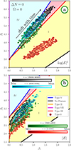Fig. 1. Uniform and unmagnetized plasma (ΔN = 0 and Ω = 0). We show β distributions of the PDFs of log|E|2 (a) and |E| (b) in the Pearson diagram (β1, β2), where β1 is the squared skewness and β2 is the kurtosis. The arrow indicates that as time advances, skewness and kurtosis increase. The legends in panel (b) list the time intervals [t0, t0 + ΔT] used to calculate the PDFs ($\mathrm{\Delta }T=2000{\omega }_{\mathrm{p}}^{-1})$ and indicate the different types of Pearson distributions; regions corresponding to Types I, IV, and VI are indicated in the map with roman numerals (see also Appendix A).

We studied the impact of Ω and ΔN on the β distributions of the PDFs of log|E|² and |E|. Figure 2a shows the β distributions (log|E|²) obtained for an unmagnetized plasma with different ΔN, calculated within a late time interval when wave turbulence is in a steady state. Density fluctuations weakly impact the spread of β distributions, which are slightly shifted towards β₀ when ΔN increases (β₁ and β₂ decrease but Pearson types do not change). No significant difference is observed between cases with ΔN > 0. Figures 2b–2d show the impact of magnetization by presenting β distributions for ω_c/ω_p = 0, 0.005, 0.2, 0.33, and 0.5 in plasmas with ΔN = 0, 0.025, and 0.05, respectively. The general trend is a shift in the β distributions with increasing magnetic field strength from their positions in the unmagnetized plasma case towards β₀; most remain in Type VI regions, and the rest remain in Type III, IV, and V regions. However, for high magnetic fields (Ω ≳ 0.3) and a homogeneous plasma (Fig. 2b), an additional decrease in the kurtosis (β₂) is observed, shifting the β distributions of the PDFs of log|E|² to the Type I region. Correspondingly, the β distributions of the PDFs of |E| (see Appendix B) weakly depend on plasma parameters and always remain within the Type I region. The only exceptions correspond to the largest magnetic fields, Ω = 0.33 and 0.5, in a uniform plasma, for which a visible decrease in β₂ is observed. Moreover, β distributions of log|E|² and |E| PDFs are presented in Appendix C for additional temperature ratios (T_e/T_i) and beam velocities (v_b/c), showing that Pearson patterns remain quasi-similar when varying these parameters in the ranges 0.3 ≤ T_e/T_i ≤ 10 and 0.08 ≤ v_b/c ≤ 0.25.

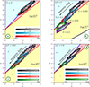Fig. 2. β distributions of the PDFs of log|E|2 represented in Pearson diagrams for different values of ΔN ≤ 0.05 and Ω ≤ 0.5, in the time interval $[t_0,t_0+\mathrm{\Delta }T]=[13000,15000]{\omega }_{\mathrm{p}}^{-1}$. Panel (a): ΔN = 0, 0.025 and 0.05 (see legend), with Ω = 0. Panel (b): Ω = 0, 0.005, 0.2, 0.33, and 0.5 (see labels), with ΔN = 0. Panel (c): Ω = 0, 0.02, 0.07, and 0.14 (see legend), with ΔN = 0.025. Panel (d): Ω = 0, 0.02, 0.07, and 0.14 (see legend), with ΔN = 0.05. The arrows indicate that skewness and kurtosis decrease when the magnetic field strength increases.

4. Analysis of Solar Orbiter observations

Let us compare our results with actual solar wind measurements. For this, we used datasets from the Time Domain Sampler (TDS) receiver (Soucek et al. 2021) of the Radio and Plasma Waves (RPW) instrument (Maksimovic et al. 2020) on board Solar Orbiter. The RPW-TDS provides regular measurements of electric field waveforms at sampling rates of 262 kHz or 524 kHz, resolving plasma waves near ω_p. Figures 3a and 3b show β distributions of the PDFs of |E| and log|E|² obtained with all waveforms recorded throughout one day, as well as an example of simulated (red lines) and observed (green dots) PDFs. The parameters β₁ and β₂ of the PDFs were calculated for the 1813 electric field snapshots with durations of 62 ms each. For comparison, we superimpose the contour boundaries of the β distributions obtained for the simulation with ΔN = 0.025 and Ω = 0.01, parameters that are close to those of the solar wind during Solar Orbiter’s data registration. Many (but not all) full-day satellite-derived β distributions show patterns in agreement with our results. Note that the PDFs of log|E|² and |E| in Fig. 3b exhibit negative and positive skewness, respectively.

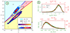Fig. 3. Panel (a): β distributions of the PDFs of |E| and log|E|2 (see legend) for waveforms provided by the RPW-TDS receiver on board Solar Orbiter, with the sampling rate 262 kHz (on January 17, 2023). Contour boundaries of β distributions obtained using waveforms provided by a simulation with ΔN = 0.025 and Ω = 0.01 are superimposed; black and cyan contours correspond to the β distributions of the PDFs of log|E|2 and |E|, respectively. Panel (b): Example of PDFs measured by Solar Orbiter (green dots) and calculated by the simulation with ΔN = 0.025 and Ω = 0.01 (red lines) at positions in the Pearson diagram indicated by a black dot (log|E|2) and a black star (|E|), respectively (see legend).

5. Discussion and conclusion

For the first time, the PDFs of |E| and log|E|² and their corresponding Pearson β distributions have been calculated by using a large number of waveforms provided by long-term 2D PIC simulations of high spatial and temporal resolutions. We studied the dependence of skewness and kurtosis on plasma magnetization (Ω), the temperature ratio T_e/T_i, the average level of density fluctuations (ΔN), and beam velocity (v_b/c). Our results show that the β distributions corresponding to log|E|² PDFs mainly belong to Type VI Pearson diagram regions, penetrating slightly into Type I and IV regions through the Type III and V lines. They are shifted to the Type I region only for homogeneous plasmas with large Ω values (≳0.3). Increasing Ω mainly leads to shifts in β distributions towards the log-normal distribution, for both homogeneous and randomly inhomogeneous plasmas. At the same time, the β distributions of the |E| PDFs mainly lie in the Type I region for the ranges of parameters considered, i.e. Ω ≤ 0.5, ΔN ≤ 0.05, 0.3 ≤ T_e/T_i ≤ 10, and 0.08 ≤ v_b/c ≤ 0.25.

Moreover, the β distributions obtained by PIC simulations are in good agreement with those calculated for the first time on the basis of high-frequency measurements by the Solar Orbiter spacecraft. Both indicate that most distributions are not log-normal, as also stated in some previous studies that analysed space data (Krasnoselskikh et al. 2007; Musatenko et al. 2007; Maksimovic et al. 2011; Vidojevic et al. 2011; Vidojevic 2014). Indeed, the distributions mostly demonstrate larger skewness and kurtosis levels than Gaussian ones, revealing specific features connected with anisotropy, flatness and peakedness, which are the signatures of various physical processes at work in upper-hybrid wave turbulence. Combining our statistical analyses with complementary diagnostics used in our previous works should lead to a better understanding of their role in the dynamics of electrostatic wave turbulence generated by electrons beams. Additionally, the dependence of the β distributions on the plasma magnetic field strength (revealed from log|E|² PDFs) can serve as a tool for the latter’s indirect estimation.

Compared to previous studies that used space measurements, we were able to generate a larger number of long-term waveforms for various beam and plasma parameters, and to estimate Pearson parameters with good accuracy, for solar wind plasmas between ∼0.05 and 1 au. Such studies will be of great help in analysing and interpreting future spacecraft measurements. Our forthcoming works will be devoted to understanding the physical processes governing wave turbulence, by studying anisotropic features as well as tail formation and shapes for a large dataset of electric field distributions.

Acknowledgments

This work was granted access to the HPC computing and storage resources under the allocation 2023-A0130510106 and 2024-A017051010 made by GENCI. This research was also financed in part by the French National Research Agency (ANR) under the project ANR-23-CE30-0049-01. C.K. thanks the International Space Science Institute (ISSI) in Bern through ISSI International Team project No. 557, Beam-Plasma Interaction in the Solar Wind and the Generation of Type III Radio Bursts. C. K. thanks the Institut Universitaire de France (IUF). Solar Orbiter is a mission of international cooperation between ESA and NASA, operated by ESA. The RPW instrument has been designed and funded by CNES, CNRS, the Paris Observatory, The Swedish National Space Agency, ESA-PRODEX and all the participating institutes.

References

Appendix A: Elements of probability theory

In this section we provide a brief summary of the key concepts of probability theory that were used in this work. We also present different types of PDFs according to the Pearson classification.

A.1. Moments of distributions

For quantitative characterization of probability density distributions, such quantities as moments are used. They can be calculated by integrating the corresponding degrees of a random variable. For a continuous distribution with density function f(x) we have

$$\begin{array}{c}\hfill {\mu }_n^{\prime }={\displaystyle \underset{-\infty }{\overset{\infty }{\int }}}{x}^{n}f(x)dx,\end{array}$$(A.1)

and for a discrete distribution with probability function p(x),

$$\begin{array}{c}\hfill {\mu }_n^{\prime }={\displaystyle \sum _x}{x}^{n}p(x).\end{array}$$(A.2)

The n^th raw moment (i.e., moment around zero) of a random variable X is denoted by E[Xⁿ]. The n^th moment of a real continuous random variable with density function f(x) around the value c is given by

$$\begin{array}{c}\hfill {\mu }_n={\displaystyle \underset{-\infty }{\overset{\infty }{\int }}}{(x-c)}^{n}f(x)dx\equiv \mathrm{E}\left[{(X-c)}^n\right].\end{array}$$(A.3)

Let us discuss the meaning of the first four moments. The first raw moment is the expected value E[X] (also called expectation or mean). In practice, the mathematical expectation is usually estimated as the arithmetic mean of the observed values of a random variable. It is proved that under some special conditions (if the sample is random, i.e. if observations are independent), the sample mean tends to the true value of the mathematical expectation of a random variable when the sample size (number of measurements) tends to infinity. For higher orders, central moments around the random variable’s mean are generally used,

$$\begin{array}{c}\hfill {\mu }_n=\mathrm{E}\left[{(X-\mu )}^n\right],\end{array}$$(A.4)

where μ ≡ μ₀′. The second central moment, which is called variance, is the expected value of the squared deviation from the mean of X:

$$\begin{array}{c}\hfill \text{Var}\left[X\right]\equiv {\mu }_2=\mathrm{E}\left[{(X-\mu )}^2\right].\end{array}$$(A.5)

Variance is a measure of dispersion, i.e. the difference between a set of numbers and its mean. Standard normalization is used for the third and fourth moments. The standardized (normalized) moment of degree n is ${\stackrel{\sim }{\mu }}_n={\mu }_n/{\sigma }^n$, where σⁿ is the n^th power of the standard deviation (the square root of the variance):

$$\begin{array}{c}\hfill {\sigma }^n={\mu }_2^{n/2}={\left(\mathrm{E}\left[{(X-\mu )}^2\right]\right)}^{n/2}.\end{array}$$(A.6)

The normalized third central moment is called skewness:

$$\begin{array}{c}\hfill \text{Skew}\left[X\right]\equiv {\stackrel{\sim }{\mu }}_3=\frac{{\mu }_3}{{\sigma }^3}=\frac{\mathrm{E}\left[{(X-\mu )}^3\right]}{{\left(\mathrm{E}\left[{(X-\mu )}^2\right]\right)}^{3/2}}.\end{array}$$(A.7)

For a distribution with a single peak (unimodal), negative (positive) skewness indicates the presence of a tail on its left (right) side, as shown by the blue (green) line in Fig. A.1a. Zero skewness means that tails on either side of the mean are balanced. This is the case for a normal distribution (brown dashed line in Fig. A.1a).

The normalized fourth central moment is called kurtosis:

$$\begin{array}{c}\hfill \text{Kurt}\left[X\right]\equiv {\stackrel{\sim }{\mu }}_4=\frac{{\mu }_4}{{\sigma }^4}=\frac{\mathrm{E}\left[{(X-\mu )}^4\right]}{{\left(\mathrm{E}\left[{(X-\mu )}^2\right]\right)}^2}.\end{array}$$(A.8)

For applications, the excess kurtosis, equal to ${\stackrel{\sim }{\mu }}_4-3$, is often used. Kurtosis represents the degree of peakedness or flatness of a distribution. For the normal distribution, the kurtosis is equal to 3 (and to 0 for the excess kurtosis). Such distributions are referred to as Mesokurtic. The two other types of distributions with kurtosis above or below 3 (so-called Leptokurtic and Platykurtic) are represented in Fig. A.1b.

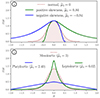Fig. A.1. Comparison of the normal distribution (dashed brown lines and coloured surface) with distributions with positive and negative skewness, ${\stackrel{\sim }{\mu }}_3$ (a) and with distributions with kurtosis ${\stackrel{\sim }{\mu }}_4$ above or below 3 (b).

A.2. Pearson distributions

The Pearson classification of random variables’ distributions is based on the Pearson differential equation

$$\begin{array}{c}\hfill \frac{df(x)}{\mathit{dx}}=-\frac{(x-a)f(x)}{b_2+b_1(x-a)+b_0{(x-a)}^2},\end{array}$$(A.9)

which specifies a family of distributions depending on the PDF f(x), the location parameter a, and the coefficients b₀, b₁, and b₂ defining the shape of the distribution.

Pearson classification is based on two main coefficients, i.e. the square of the skewness, ${\beta }_1={\stackrel{\sim }{\mu }}_3^2$, and the kurtosis, ${\beta }_2={\stackrel{\sim }{\mu }}_4$. Each distribution can be represented by a single point in the Pearson diagram, i.e. in the (β₁, β₂) map (Fig. A.2). Many widely used distributions are special cases of Pearson distributions, for example Beta distribution (Type I), Cauchy distribution (Type IV), continuous uniform distribution (limit of Type I), exponential distribution and Gamma distribution (Type III), inverse-gamma distribution (Type V), Normal distribution (limit case of many types), and Student’s t-distribution (Type VII).

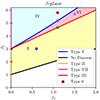Fig. A.2. Pearson diagram showing the points (β1, β2) corresponding to the distributions of Types I to VII presented in Figs. A.3–A.6.

Figures A.3–A.6 show different types of Pearson distributions (solid colour lines) compared with the normal distribution (dashed brown lines), in logarithmic scale. Each distribution corresponds to a dot of same colour in Fig. A.2.

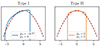Fig. A.3. Type I and Type II Pearson distributions.

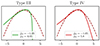Fig. A.4. Type III and Type IV Pearson distributions.

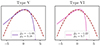Fig. A.5. Type V and Type VI Pearson distributions.

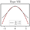Fig. A.6. Type VII Pearson distribution.

Appendix B: Distributions of the PDFs of |E|

Figure B.1 shows the β distributions of the PDFs of the electric field amplitudes (|E|) as a function of ΔN = 0, 0.025, 0.05 for Ω = 0 (a) and, at fixed ΔN = 0, 0.025, 0.05, for various values of Ω (b-d). All these distributions slightly differ one from the other, except those corresponding to homogeneous plasmas with Ω = 0.33 and Ω = 0.5 in panel (b).

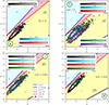Fig. B.1. β distributions of the PDFs of |E|, in the Pearson diagram, for different values of ΔN ≤ 0.05 and Ω ≤ 0.5, in the time interval [t0, t0 + ΔT]=[13000, 15000]ωp−1. Panel (a): ΔN = 0, 0.025, and 0.05 (see legend), with Ω = 0. Panel (b): Ω = 0, 0.005, 0.2, 0.33 and 0.5 (see labels), with ΔN = 0. Panel (c): Ω = 0, 0.02, 0.07, and 0.14 (see legend), with ΔN = 0.025. Panel (d): Ω = 0, 0.02, 0.07, and 0.14 (see legend), with ΔN = 0.05.

Appendix C: Impact of the temperature ratio and beam velocity

The characteristic pattern of β distributions found for two simulations with temperature ratios (beam velocities) in the range 0.3 ≤ T_e/T_i ≤ 10 (0.08 ≤ v_b/c ≤ 0.25) are shown in Figs. C.1, C.2, C.3, and C.4, for T_e = 0.3T_i, T_e = 3T_i, v_b = 0.18c, and v_b = 0.08c, respectively. We observe that the β distributions corresponding to the PDFs of log|E|² and |E| belong to the same Pearson Types as found in Figs. 1-3 and B.1.

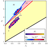Fig. B.2. β distributions of the PDFs of |E| and log|E|2 in the Pearson diagram, for Te = 0.3Ti, ΔN = 0, Ω = 0, and vb = 0.25c, in the range $[t_0,t_0+\mathrm{\Delta }T]=[13000,15000]{\omega }_p^{-1}$. One can compare, for similar parameters, with Figs. 2a and B.1a, where Te/Ti = 10.

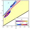Fig. B.3. β distributions of the PDFs of |E| and log|E|2 in the Pearson diagram, for Te = 3Ti, ΔN = 0, Ω = 0, and vb = 0.25c, in the range $[t_0,t_0+\mathrm{\Delta }T]=[13000,15000]{\omega }_p^{-1}$. One can compare, for similar parameters, with Figs. 2a and B.1a, where Te/Ti = 10.

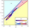Fig. B.4. β distributions of the PDFs of |E| and log|E|2 in the Pearson diagram, for vb = 9vT ≃ 0.18c, ΔN = 0.05, Ω = 0.07, and Te/Ti = 10, in the range $[t_0,t_0+\mathrm{\Delta }T]=[13000,15000]{\omega }_p^{-1}$. One can compare, for similar parameters, with Figs. 2d and B.1d, where vb = 0.25c.

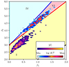Fig. B.5. β distributions of the PDFs of |E| and log|E|2 in the Pearson diagram, for Te = 3Ti, vb = 12.7vT ≃ 0.08c, ΔN = 0.025 and Ω = 0.02, in the range $[t_0,t_0+\mathrm{\Delta }T]=[8000,10000]{\omega }_p^{-1}$. One can compare, for similar parameters, with Figs. 2c and B.1c, where vb = 0.25c and Te/Ti = 10.

All Figures

Fig. 1. Uniform and unmagnetized plasma (ΔN = 0 and Ω = 0). We show β distributions of the PDFs of log|E|2 (a) and |E| (b) in the Pearson diagram (β1, β2), where β1 is the squared skewness and β2 is the kurtosis. The arrow indicates that as time advances, skewness and kurtosis increase. The legends in panel (b) list the time intervals [t0, t0 + ΔT] used to calculate the PDFs ($\mathrm{\Delta }T=2000{\omega }_{\mathrm{p}}^{-1})$ and indicate the different types of Pearson distributions; regions corresponding to Types I, IV, and VI are indicated in the map with roman numerals (see also Appendix A).

In the text

Fig. 2. β distributions of the PDFs of log|E|2 represented in Pearson diagrams for different values of ΔN ≤ 0.05 and Ω ≤ 0.5, in the time interval $[t_0,t_0+\mathrm{\Delta }T]=[13000,15000]{\omega }_{\mathrm{p}}^{-1}$. Panel (a): ΔN = 0, 0.025 and 0.05 (see legend), with Ω = 0. Panel (b): Ω = 0, 0.005, 0.2, 0.33, and 0.5 (see labels), with ΔN = 0. Panel (c): Ω = 0, 0.02, 0.07, and 0.14 (see legend), with ΔN = 0.025. Panel (d): Ω = 0, 0.02, 0.07, and 0.14 (see legend), with ΔN = 0.05. The arrows indicate that skewness and kurtosis decrease when the magnetic field strength increases.

In the text

Fig. 3. Panel (a): β distributions of the PDFs of |E| and log|E|2 (see legend) for waveforms provided by the RPW-TDS receiver on board Solar Orbiter, with the sampling rate 262 kHz (on January 17, 2023). Contour boundaries of β distributions obtained using waveforms provided by a simulation with ΔN = 0.025 and Ω = 0.01 are superimposed; black and cyan contours correspond to the β distributions of the PDFs of log|E|2 and |E|, respectively. Panel (b): Example of PDFs measured by Solar Orbiter (green dots) and calculated by the simulation with ΔN = 0.025 and Ω = 0.01 (red lines) at positions in the Pearson diagram indicated by a black dot (log|E|2) and a black star (|E|), respectively (see legend).

In the text

	Fig. A.1. Comparison of the normal distribution (dashed brown lines and coloured surface) with distributions with positive and negative skewness, ${\stackrel{\sim }{\mu }}_3$ (a) and with distributions with kurtosis ${\stackrel{\sim }{\mu }}_4$ above or below 3 (b).
In the text

	Fig. A.2. Pearson diagram showing the points (β1, β2) corresponding to the distributions of Types I to VII presented in Figs. A.3–A.6.
In the text

	Fig. A.3. Type I and Type II Pearson distributions.
In the text

	Fig. A.4. Type III and Type IV Pearson distributions.
In the text

	Fig. A.5. Type V and Type VI Pearson distributions.
In the text

	Fig. A.6. Type VII Pearson distribution.
In the text

Fig. B.1. β distributions of the PDFs of |E|, in the Pearson diagram, for different values of ΔN ≤ 0.05 and Ω ≤ 0.5, in the time interval [t0, t0 + ΔT]=[13000, 15000]ωp−1. Panel (a): ΔN = 0, 0.025, and 0.05 (see legend), with Ω = 0. Panel (b): Ω = 0, 0.005, 0.2, 0.33 and 0.5 (see labels), with ΔN = 0. Panel (c): Ω = 0, 0.02, 0.07, and 0.14 (see legend), with ΔN = 0.025. Panel (d): Ω = 0, 0.02, 0.07, and 0.14 (see legend), with ΔN = 0.05.

In the text

	Fig. B.2. β distributions of the PDFs of |E| and log|E|2 in the Pearson diagram, for Te = 0.3Ti, ΔN = 0, Ω = 0, and vb = 0.25c, in the range $[t_0,t_0+\mathrm{\Delta }T]=[13000,15000]{\omega }_p^{-1}$. One can compare, for similar parameters, with Figs. 2a and B.1a, where Te/Ti = 10.
In the text

	Fig. B.3. β distributions of the PDFs of |E| and log|E|2 in the Pearson diagram, for Te = 3Ti, ΔN = 0, Ω = 0, and vb = 0.25c, in the range $[t_0,t_0+\mathrm{\Delta }T]=[13000,15000]{\omega }_p^{-1}$. One can compare, for similar parameters, with Figs. 2a and B.1a, where Te/Ti = 10.
In the text

	Fig. B.4. β distributions of the PDFs of |E| and log|E|2 in the Pearson diagram, for vb = 9vT ≃ 0.18c, ΔN = 0.05, Ω = 0.07, and Te/Ti = 10, in the range $[t_0,t_0+\mathrm{\Delta }T]=[13000,15000]{\omega }_p^{-1}$. One can compare, for similar parameters, with Figs. 2d and B.1d, where vb = 0.25c.
In the text

	Fig. B.5. β distributions of the PDFs of |E| and log|E|2 in the Pearson diagram, for Te = 3Ti, vb = 12.7vT ≃ 0.08c, ΔN = 0.025 and Ω = 0.02, in the range $[t_0,t_0+\mathrm{\Delta }T]=[8000,10000]{\omega }_p^{-1}$. One can compare, for similar parameters, with Figs. 2c and B.1c, where vb = 0.25c and Te/Ti = 10.
In the text

References

- Annenkov, V. 2025, A&A, 693, A236 [NASA ADS] [CrossRef] [EDP Sciences] [Google Scholar]
- Arzhannikov, A. V., Ivanov, I. A., Kasatov, A. A., et al. 2020, Plasma Phys. Control. Fusion, 62, 045002 [CrossRef] [Google Scholar]
- Bale, S. D., Burgess, D., Kellogg, P. J., Goetz, K., & Monson, S. J. 1997, J. Geophys. Res., 102, 11281 [Google Scholar]
- Burdakov, A., Avrorov, A. P., Arzhannikov, A. V., et al. 2013, Fusion Sci. Technol., 63, 29 [Google Scholar]
- Cairns, I. H., & Menietti, J. D. 2001, J. Geophys. Res., 106, 29515 [Google Scholar]
- Cairns, I. H., & Robinson, P. A. 1997, Geophys. Res. Lett., 24, 369 [Google Scholar]
- Cairns, I. H., & Robinson, P. A. 1999, Phys. Rev. Lett., 82, 3066 [Google Scholar]
- Derouillat, J., Beck, A., Pérez, F., et al. 2018, Comput. Phys. Commun., 222, 351 [NASA ADS] [CrossRef] [Google Scholar]
- Fisher, R. 1912, Messenger Math., 41, 155 [Google Scholar]
- Fox, N. J., Velli, M. C., Bale, S. D., et al. 2016, Space Sci. Rev., 204, 7 [Google Scholar]
- Ginzburg, V. L., & Zheleznyakov, V. V. 1958, Sov. Astron., 2, 653 [NASA ADS] [Google Scholar]
- Hoppe, M., Ekmark, I., Berger, E., & Fülöp, T. 2022, J. Plasma Phys., 88 [CrossRef] [Google Scholar]
- Krafft, C., & Savoini, P. 2021, ApJ, 917, L23 [NASA ADS] [CrossRef] [Google Scholar]
- Krafft, C., & Savoini, P. 2022a, ApJ, 924, L24 [NASA ADS] [CrossRef] [Google Scholar]
- Krafft, C., & Savoini, P. 2022b, ApJ, 934, L28 [Google Scholar]
- Krafft, C., & Savoini, P. 2023, ApJ, 949, 24 [NASA ADS] [CrossRef] [Google Scholar]
- Krafft, C., & Savoini, P. 2024, ApJ, 964, L30 [NASA ADS] [CrossRef] [Google Scholar]
- Krafft, C., Volokitin, A. S., & Gauthier, G. 2019, Fluids, 4, 69 [Google Scholar]
- Krafft, C., Savoini, P., & Polanco-Rodríguez, F. J. 2024, ApJ, 967, L20 [Google Scholar]
- Krasnoselskikh, V. V., Lobzin, V. V., Musatenko, K., et al. 2007, J. Geophys. Res., 112, A10109 [Google Scholar]
- Li, B., Cairns, I. H., Robinson, P. A., LaBelle, J., & Kletzing, C. A. 2010, Phys. Plasma, 17, 032110 [Google Scholar]
- Maksimovic, M., Vidojevic, S., & Zaslavsky, A. 2011, Baltic Astron., 20, 600 [Google Scholar]
- Maksimovic, M., Bale, S. D., Chust, T., et al. 2020, A&A, 642, A12 [EDP Sciences] [Google Scholar]
- Müller, D., Cyr, O. C. S., Zouganelis, I., et al. 2020, A&A, 642, A1 [NASA ADS] [CrossRef] [EDP Sciences] [Google Scholar]
- Musatenko, K., Lobzin, V., Soucek, J., Krasnoselskikh, V., & Décréau, P. 2007, Planet. Space Sci., 55, 2273 [Google Scholar]
- Pearson, K. 1895, Philos. Trans. R. Soc. London, Ser. A, 186, 343 [Google Scholar]
- Polanco-Rodríguez, F. J., Krafft, C., & Savoini, P. 2025, ApJ, 982, L24 [Google Scholar]
- Reid, H. A. S., & Kontar, E. P. 2017, A&A, 598, A44 [NASA ADS] [CrossRef] [EDP Sciences] [Google Scholar]
- Reid, H. A. S., & Ratcliffe, H. 2014, Res. Astron. Astrophys., 14, 773 [Google Scholar]
- Robinson, P. A. 1993, Sol. Phys., 146, 357 [Google Scholar]
- Robinson, P. A., & Cairns, I. H. 2000, Geophys. Monogr. Ser., 119, 37 [Google Scholar]
- Soldatkina, E., Pinzhenin, E., Korobeynikova, O., et al. 2022, Nucl. Fusion, 62, 066034 [Google Scholar]
- Soucek, J., Píša, D., Kolmasova, I., et al. 2021, A&A, 656, A26 [CrossRef] [EDP Sciences] [Google Scholar]
- Vidojevic, S. 2014, Adv. Space Res., 54, 1326 [Google Scholar]
- Vidojevic, S., Zaslavsky, A., Maksimovic, M., Dražic, M., & Atanackovic, O. 2011, Baltic Astron., 20, 596 [Google Scholar]
- Voshchepynets, A., Volokitin, A., Krasnoselskikh, V., & Krafft, C. 2017, J. Geophys. Res., 122, 3915 [Google Scholar]