| Issue |
A&A
Volume 699, July 2025
|
|
|---|---|---|
| Article Number | A146 | |
| Number of page(s) | 12 | |
| Section | Stellar structure and evolution | |
| DOI | https://doi.org/10.1051/0004-6361/202555003 | |
| Published online | 04 July 2025 | |
Angular momentum relaxation in models of rotating early-type stars
1
IRAP, Université de Toulouse, CNRS, CNES, 14, avenue Édouard Belin, F-31400 Toulouse, France
2
ISAE-SUPAERO, Université de Toulouse, F-31400 Toulouse, France
3
Université Paris-Saclay, Université de Paris, Sorbonne Paris Cité, CEA, CNRS, AIM, F-91191 Gif-sur-Yvette, France
⋆ Corresponding authors: Michel.Rieutord@irap.omp.eu; Enzo.Brossier-Secher@student.isae-supaero.fr; Joey.Mombarg@cea.fr
Received:
2
April
2025
Accepted:
14
May
2025
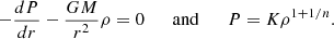
Context. The rotational evolution of stars remains an open question in stellar physics because numerous phenomena contribute to the distribution of angular momentum.
Aims. This paper aims to determine the timescale over which a rotating early-type star relaxes to a steady baroclinic state or, equivalently, the conditions under which its nuclear evolution is slow enough to allow the star's evolution to be modelled as a series of quasi-steady states.
Methods. We investigate the damping timescale of baroclinic and viscous eigenmodes that are potentially excited by the continuous forcing of nuclear evolution. We first examine this with a spherical Boussinesq model. Since much of the dynamics is concentrated in the radiative envelope of the star, we then improve the realism of the modelling by using a polytropic model of the envelope that incorporates a realistic density profile.
Results. The polytropic model of the envelope highlights the key role of the region at the core-envelope interface. The results of evolutionary models recently obtained with two-dimensional axisymmetric ESTER models appear to arise from the slow damping of viscous modes. Using a vanishing Prandtl number appears to be too strong an approximation to explain the models’ dynamics. Baroclinic modes, previously thought to be good candidates for this relaxation process, are found to be too rapidly damped.
Conclusions. The dynamical response of rotating stars to the slow forcing of their nuclear evolution appears as a complex combination of non-oscillating eigenmodes. Simple Boussinesq approaches are not sufficiently realistic to explain this reality. This study underlines the key role of layers near the core-envelope interface in early-type stars as well as the importance of angular momentum transport mechanisms-here represented by viscosity-for early-type stars to reach critical rotation, which is presumably associated with the Be phenomenon.
Key words: stars: early-type / stars: evolution / stars: rotation
© The Authors 2025
 Open Access article, published by EDP Sciences, under the terms of the Creative Commons Attribution License (https://creativecommons.org/licenses/by/4.0), which permits unrestricted use, distribution, and reproduction in any medium, provided the original work is properly cited.
This article is published in open access under the Subscribe to Open model. Subscribe to A&A to support open access publication.
1. Introduction
Rotation is part of the dynamical evolution of a star. In intermediate-mass stars, where neither magnetic braking nor winds extract a substantial amount of angular momentum, main-sequence stars tend to evolve towards critical rotation and may form an excretion disc, which can explain the Be phenomenon Ekström et al. (2008), Granada et al. (2013), Hastings et al. (2020). However, simulations of the time evolution of rapidly rotating stars using recent two-dimensional, wind-free ESTER models Mombarg et al. (2024) show that stars above 7 M⊙, never approach critical rotation, regardless of their initial rotation rate (tested up to 90% of the critical value).
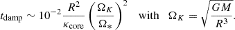
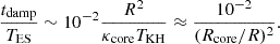
Mombarg et al. (2024) proposed that nuclear evolution is too rapid for the star to redistribute its angular momentum. Indeed, as the star evolves, driven by nuclear reactions in its core, it inflates, and thus the angular momentum is redistributed by transient flows. If such a forcing is sufficiently slow, the star follows a sequence of quasi-steady states at constant total angular momentum, approaching critical rotation (e.g. Gagnier et al. 2019). However, when nuclear evolution is rapid, the star cannot relax to the quasi-steady state, presumably because excited eigenmodes are not damped quickly enough. Following the work of Busse (1981, 1982), Mombarg et al. (2024) suggests that these eigenmodes are baroclinic modes, which can be viewed as non-oscillating gravito-inertial modes whose characteristic damping timescale is the Eddington-Sweet timescale. This timescale is typically evaluated by the Kelvin-Helmholtz time divided by the centrifugal flattening of the star. According to this criterion, and considering models rotating at 75% of the break-up velocity, the damping timescale of baroclinic modes should be shorter than the nuclear timescale (e.g. Gagnier et al. 2019), even for a 10 M⊙ star. This estimate is based on orders of magnitude, and non-dimensional factors may alter this conclusion.
The present work therefore aims to clarify this question by investigating the properties of baroclinic modes in a more realistic setup than that of Busse, who analysed a simple horizontal plane layer using the Boussinesq approximation with a vanishing viscosity.
This article is organised as follows. In Sect. 2, we present a more detailed presentation of baroclinicity in stars. In Sect. 3. we analyse baroclinic modes in a rotating sphere using the Boussinesq approximation. In Sect. 4 we address the limitations of the Boussinesq model and discuss a more realistic model using a polytropic, stably stratified, rotating spherical layer that mimics the radiative envelope of an early-type star. In Sect. 5, we discuss the results in terms of timescales, clarifying the role of viscosity. Conclusions follow.
2. The baroclinic state of rotating stars
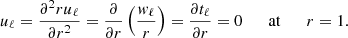
To address the questions raised by baroclinic modes, it is useful to recall the origin of baroclinicity in rotating stars. A natural starting point is gravity darkening.
Gravity darkening was first described a century ago by von Zeipel, who studied radiative equilibrium in rotating stars (von Zeipel 1924). Gravity darkening refers to the reduction in heat flux from pole to equator at the surface of a rotating star. This effect is a simple consequence of centrifugal flattening and the Fourier law: because the distance from the centre to the equator is greater than to the pole, the temperature gradient is smaller at equator than along the polar axis, and hence the heat flux is larger at the poles than at the equator. A more detailed discussion can be found in Espinosa Lara & Rieutord (2011).
An intuitive consequence of gravity darkening is that temperature is generally not constant on isobars. This is termed baroclinicity; in other words, the three gradients of pressure, density and temperature-namely ∇P, ∇ρ, and ∇T-are inclined to one another. To preserve hydrostatic equilibrium, von Zeipel (1924) suggested that heat sources within the star obey the relation  , where Ω* is the rotation rate and G the gravitational constant. Eddington (1925) was rightly sceptical of this relation, which would, from a modern perspective, constrain microphysics with fundamental stellar parameters. He proposed that the resulting thermal imbalance would simply break hydrostatic equilibrium. Eddington believed this would result in a meridional circulation, an idea that later gave rise to the erroneous concept of the Eddington-Sweet circulation (Sweet 1950). Unfortunately, this concept persisted for many decades (Kippenhahn & Weigert 1990). A more detailed treatment of this issue can be found in work of Busse (1981, 1982) and the lecture notes of Rieutord et al. (2006). At present, 2D numerical models of rapidly rotating stars have established the solution (Espinosa Lara & Rieutord 2013): in a steady state, as Eddington (1925) proposed, there is indeed no hydrostatic equilibrium, but rather a baroclinic flow consisting of differential rotation and a weak meridional circulation. This meridional circulation vanishes in the absence of viscosity (e.g. Espinosa Lara & Rieutord 2013). This occurs because, in a steady state, the angular momentum flux is zero through any closed surface. Since differential rotation in a viscous fluid induces an angular momentum flux by viscous friction, it must be compensated by a meridional circulation (e.g. Rieutord et al. 2006; Espinosa Lara & Rieutord 2013; Gagnier & Rieutord 2020).
As noted in the introduction, we seek to determine how long it takes to establish such a differential rotation. In other words, if a process such as nuclear evolution perturbs the steady state, on what timescale does the rotating star relax?
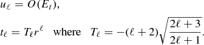
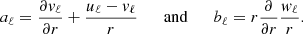
Busse (1981) identified the relaxation process as being primarily controlled by the damping of baroclinic modes. However, he investigated this problem using a very simple model consisting of a horizontal plane fluid layer, whose perturbations are treated using the Boussinesq approximation and assuming vanishing viscosity. For general initial conditions, this model shows that both gravito-inertial and baroclinic modes are simultaneously excited. The former are damped on the usual thermal timescale, d2/κ*, where d is the thickness of the layer, and κ* is the heat diffusivity. In contrast, baroclinic modes are damped on the timescale  , where N* is the Brunt-Väisälä frequency and Ω* the angular velocity. This new timescale can be compared to the Eddington-Sweet timescale in terms of orders of magnitude (Busse 1981; Zahn 1992). When rotation is slow, the Eddington-Sweet timescale is much longer than the diffusion timescale. Quantitatively, the key result of Busse's analysis is that the least-damped baroclinic mode has a damping rate given by
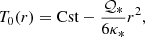
where R is the stellar radius. This expression is obtained by adapting the analytic expression of the damping rate derived for the horizontal plane model to a radius sphere R. However, applying this formula to a real star is risky, given the strong simplifications imposed by Busse's modelling. For instance, quantities such as thermal diffusivity κ* or the Brunt-Väisälä frequency N* vary by orders of magnitude inside a star. Hence, if the scaling is correct, it remains unclear which value should be used for these parameters.
To address this issue, we therefore consider more realistic models, first by including the spherical geometry of the star, then by accounting for the strong variations of heat diffusivity associated with density variations, and finally by examining the role of viscosity.
3. The spherical Boussinesq model
As a first step, and to extend Busse's result, we consider a self-gravitating, rotating sphere of quasi-incompressible fluid, whose perturbations are treated using the Boussinesq approximation. In essence, we revisit the model of Dintrans et al. (1999), which is a simplified model of a star. This type of model has been widely employed since the seminal work of Chandrasekhar (1961). However, while Dintrans et al. (1999) focused on the gravito-inertial modes of a spherical shell, they did not investigate the baroclinic modes, which are the subject of the present study.
3.1. Mathematical formulation
Following Dintrans et al. (1999), we adopt (2Ω*)−1 as a timescale and the radius of the sphere R as a length scale. To impose a stable stratification, we introduce uniformly distributed heat sinks of power  . The background temperature field then satisfies
with boundary conditions imposing regularity at the centre of the sphere and a fixed temperature at the surface. The spherically symmetric solution is
where r is the radial spherical coordinate. We define β=∂rT0 as the temperature gradient of the fluid. Since  , it is positive if
  . We adopt βR as the temperature scale for temperature perturbations. Under the Boussinesq approximation, gravity takes the form g=−g0r/R, where g0 is the surface gravity.
Using this scaling, the non-dimensional linearised equations governing perturbations of the hydrostatic equilibrium in a rotating frame (neglecting centrifugal acceleration) are:
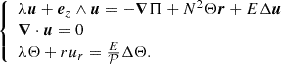
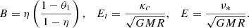
These represent, respectively, the conservation of momentum, mass, and energy, with u the non-dimensional velocity field and Θ the perturbation temperature field. The reduced pressure perturbation is denoted by Π. We assume a time dependence of all perturbations of the form exp(λτ), where λ is the non-dimensional eigenvalue characterising the associated eigenmode. We also introduced non-dimensional constants:
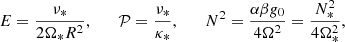
where E is the Ekman number, which measures the kinematic viscosity, ν*,  is the Prandtl number, and N* is the dimensional Brunt-Väisälä frequency. The dilation coefficient at constant pressure is denoted by α.
To solve the above partial differential equations, we need boundary conditions. For the velocity field, we adopt stress-free boundary conditions:
![$$ {{{{\boldsymbol {{u}}}}}}\cdot { {{\boldsymbol {{e}}}}_r}= {{{{\boldsymbol {{0}}}}}}{ \qquad {\mathrm {and}}\qquad }{ {{\boldsymbol {{e}}}}_r}\times ([\sigma ] { {{\boldsymbol {{e}}}}_r}) = {{{{\boldsymbol {{0}}}}}}, $$](/articles/aa/full_html/2025/07/aa55003-25/aa55003-25-eq12.gif)
on the surface of the sphere at r = 1. In this expression [σ] is the stress tensor. For the temperature, we assume that the surface is a perfect insulator, or equivalently, that the surface heat flux is fixed, so that

3.2. Properties of solutions
3.2.1. Preliminaries
Equation (4), together with boundary conditions, defines an eigenvalue problem. In the horizontal plane configuration, this problem can be solved analytically through a Fourier expansion of all fields (Busse 1981). In the present spherical geometry, variables cannot be separated, which precludes a fully analytic solution. However, Busse's results provide a useful guide for obtaining simplified expression for baroclinic modes. Since baroclinically driven differential rotation is axisymmetric and we focus on small-amplitude perturbations, we restrict our analysis to axisymmetric baroclinic modes.
We begin by expanding the disturbances in spherical harmonics, following the approach of Dintrans et al. (1999):
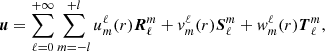
with

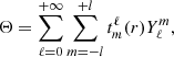
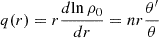
where gradients are taken on the unit sphere. Since fields are axisymmetric, we restrict the expansion to m = 0 components only and omit the m-index for clarity. The projection of equations (4) leads to a coupled system of ordinary differential equations for the radial functions tℓ,uℓ, and wℓ (vℓ is eliminated using ∇·u = 0). We find
where we introduced  , the coupling coefficients, arising from the Coriolis term, are:
The radial Laplacian is defined as
The boundary conditions for the radial functions are now:
Regularity at the centre is also imposed. The equations presented will be solved numerically. We first use these equations to derive an approximate solution for the baroclinic modes and their damping rates.
3.2.2. An asymptotic solution for the main baroclinic mode
In stars, the Prandtl number  is usually assumed to be very small, typically ≲10−4, based on the transport properties of photons. We adopt this assumption here, although we will revisit it in Sect. 4.3.2. The Ekman number is even smaller, with E≲10−12. Busse (1981) showed that baroclinic modes are non-oscillatory and are damped by thermal diffusion. In our non-dimensional set-up, thermal diffusion is represented by the ratio
  , which is also small for the above orders of magnitude. A natural simplification, also adopted by Busse, is to neglect viscosity altogether but retain thermal diffusivity. This corresponds to setting
  while keeping Et small but finite. If, in addition, the Brunt-Väisälä frequency is much larger than the Coriolis frequency, i.e. if N≫1, then a simple solution to (8) emerges:
At first order, this solution satisfies the inviscid (i.e. no-diffusion) boundary conditions, but it does not satisfy the additional surface boundary conditions in (9) that arise from viscosity or heat diffusion. To be complete, boundary layer corrections would be required. However, such corrections are not important with the chosen stress-free and insulating conditions, since these do not generate strong velocity or temperature gradients that could influence viscous or thermal dissipation (an example of such a situation is given in Rieutord & Zahn 1997).
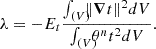
The solutions (10) and (11) describe a disturbance whose main components are δvφ and δT, that is, a perturbation of the azimuthal velocity (or the local rotation rate) and of the temperature field. The associated meridional circulation, determined by uℓ, is much smaller. Moreover, the damping rate can be derived analytically using the exact expression given by (cf Dintrans et al. 1999):
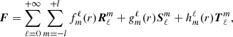
where Dvis is the viscous dissipation, Dth is the thermal dissipation, Ek is the kinetic energy, and Eth is the thermal energy of the disturbance. Using the expansion in spherical harmonics, these quantities are given by:
![$$ \begin{aligned} E_{th} &= \dfrac {N^2}{2}\sum _{\ell = 0}^\infty \int _{0}^1{{t_\ell }}^2r^2dr \\ E_k &= \dfrac {1}{2}\sum _{\ell = 0}^\infty \int _{0}^1\left [{{u_\ell }}^2 + {\ell (\ell +1)}\left ({{v_\ell }}^2 + {{w_\ell }}^2\right )\right ]r^2dr \\ D_{th} &= E_tN^2\sum _{\ell = 0}^\infty \int _{0}^1\left [\left |\dfrac {\partial {t_\ell }}{\partial r}\right |^2 + \dfrac {{\ell (\ell +1)}}{r^2}{{t_\ell }}^2\right ]r^2dr \\ D_{visc} &= E\sum _{\ell = 0}^\infty \int _{0}^1\left [3\left |\dfrac {\partial {u_\ell }}{\partial r}\right |^2 + {\ell (\ell +1)}\left (|a_\ell |^2 + |b_\ell |^2\right )\right . \\ &\qquad \qquad +\left .\ell (\ell ^2-1)(\ell +2)\dfrac {|{v_\ell }|^2 + |{w_\ell }|^2}{r^2}\right ]r^2dr, \end{aligned} $$](/articles/aa/full_html/2025/07/aa55003-25/aa55003-25-eq28.gif)
where
Using the expressions of tℓ and wℓ, the damping rate can be easily evaluated, and we find the following:
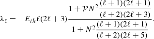
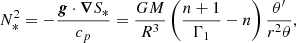
From the foregoing expression, we note that the absolute value of the damping rate is a growing function of ℓ, thus the least-damped mode is obtained for ℓ = 1. However, the associated eigenmode does not verify the equatorial symmetry of the forcing, that is, the forcing due to stellar inflation resulting from nuclear evolution. Hence, the least-damped mode excited by nuclear evolution is the one with ℓ = 2. The associated damping rate is given by:
We recall that N=N*/2Ω*, and that this value is typically ≲10 in rapidly rotating stars. For instance, using 2D-ESTER models1 (e.g. Rieutord et al. 2016), we find that a 5 M⊙ model rotating at 50% of the critical angular velocity (i.e. an equatorial velocity of ∼250 km/s) has an average N of around four. In (15), the numerator can be confidently set to unity since we assume  .
.
At low or moderate rotation 5N2/12≫1, thus
or, with dimensional quantities, to
This result is remarkably close to the prediction from the Cartesian model of Busse (1981), who finds
This result indicates a relatively simple least-damped baroclinic mode in spherical geometry. We now complete its analysis with a numerical solution of the full system (4).
3.2.3. Numerical solutions
We solve system (8) using spectral methods, as demonstrated by Dintrans et al. (1999) for gravito-inertial modes. We discretise the radial functions on a Gauss-Lobatto grid associated with Chebyshev polynomials (Fornberg 1998). We solve the generalised eigenvalue problem resulting from the discretisation of the equations using classical methods, such as the QZ-algorithm for computation of the full spectrum, or the Arnoldi-Chebyshev algorithm for the derivation of specific eigenvalues. The latter algorithm is particularly well suited to the present problem, since we have an approximation of the desired eigenvalues.
To numerically control the validity of the approximate solutions described above, we focus on the least-damped mode with the main spherical harmonic ℓ = 2. This mode is easily retrieved when N = 1, Et = 10−3, and  . We show its shape in Fig. 1. The meridional distribution of vφ (Fig. 1, middle panel) clearly agrees with the solution of (10), which suggests

or a differential rotation

The shape of this baroclinic mode shows that, when it is excited, regions near θ∼30° will accelerate, while regions near the equator decelerate (or vice versa). Hence, angular momentum is redistributed by this mode, as also shown by the shape of the meridional flow (Fig. 1, left panel). Other baroclinic modes also redistribute angular momentum, but on a smaller scale, and are damped more rapidly.
 |
Fig. 1. Meridional view of the least-damped baroclinic mode. Left: streamlines of the meridional velocity; middle: azimuthal velocity; right: temperature perturbation. In the middle and right panels, solid lines indicate the change of sign of the field. The solution is associated with the eigenvalue λ=−8.653×10⁻³ obtained with parameters E = 0, Et = 10−3, N = 1, and numerical resolution Lmax = 50, Nr = 50. |
As the central question of the present work is to estimate the timescale over which baroclinic modes are damped, we compare the numerical solution for the damping rate of the least-damped mode with the prediction given by (15). This comparison is shown in Fig. 2, where we present the evolution of the real part of the associated eigenvalue as a function of N=N*/2Ω*. We find that, when N is sufficiently large (N≳4, for example), the eigenvalue calculated from the full solution matches its approximate form given by (15) very well.
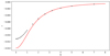 |
Fig. 2. Damping rate of the least-damped baroclinic mode in the spherical Boussinesq model as a function of the ratio N=N*/2Ω*, for |

4. The polytropic model
From the Boussinesq model, it is difficult to derive the actual timescale for damping of baroclinic modes, since thermal diffusivity and density vary by several orders of magnitude inside a star. For the previous 5 M⊙ model, central values suggest a timescale of ∼1 Myr, while surface values indicate ∼1 day. We now consider a polytropic model of the stellar envelope, which allows us to account for the strong variations in density and their impact on heat diffusivity.
4.1. Mathematical formulation
4.1.1. Background structure
Baroclinic modes are disturbances that arise from the combined effect of stable stratification and background rotation. We therefore focus on radiative envelopes. To simplify the problem, we assume that the radiative envelope is at rest in a corotating frame and that centrifugal distortion can be neglected. We also neglect the baroclinic structure of the envelope and the baroclinic flows that pervade it in a steady state. This is not an issue for baroclinic modes, which can appear on a barotropic structure, as demonstrated by the Boussinesq case. In fact, these modes are the perturbations that cause the barotropic structure to transition to a baroclinic structure. Their damping rate indicates the timescale for this transition to occur. The barotropic and baroclinic structures are not very different, so the damping rates should be almost unaffected by this change.
We further assume that the equation of state is that of a polytrope of index n, and that all the mass of the star resides in its core. Thus, the structure of the envelope is governed by
Equations (17) can be solved analytically, giving the following profiles:
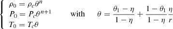
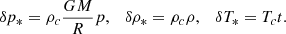
for density ρ0(r), pressure P0(r), and temperature T0(r). In the above expression, the c-index refers to the values at the core-envelope interface and η is the fractional radius of this interface. The function θ is analogous to the Lane-Emden function for the spherical layer and θ1 is the value at the surface r = 1. To characterise the density contrast of the envelope, we introduce the parameter Q, defined as
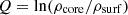
so that
For orders of magnitude in observed stars, we refer to a 5 M⊙ non-rotating ZAMS model, which represents a typical intermediate-mass star. For such a model, Q∼23.
If we neglect any heat source in the envelope, this model implies that heat conductivity, χ*, is constant2. We consider the assumption of constant χ* to be a reasonable approximation, since a realistic model of a 5 M⊙ star shows variations less than an order of magnitude over the envelope, in contrast to the thermal diffusivity, κ*=χ*/cpρ0 (see Fig. 3).
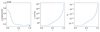 |
Fig. 3. Radial profiles of the thermal conductivity (left), thermal diffusivity (middle), and the resulting non-dimensional parameter Et (right) for a non-rotating 5 M⊙ ESTER model at the zero-age main sequence (ZAMS). |
For completeness, we also assume a constant effective kinematic viscosity, ν*, in the envelope. This parameter is difficult to estimate, as it depends on the local small-scale turbulence. To be consistent with the ESTER 2D models used by Mombarg et al. (2023), we adopt the value ν* = 107 cm2/s. This value is an estimate based on the observed differential rotation in γ Doradus stars (Mombarg 2023). By making this assumption, we imply that small-scale turbulence in radiative envelopes acts as a diffusive process of similar magnitude for either scalars (chemicals) and vectors (momentum), as detailed in the discussion.
Finally, we treat the convective core as a rigidly rotating sphere because of its high turbulent viscosity.
Although this model is approximate, it has several advantages: it is analytical and therefore not sensitive to numerical errors; it captures the key variations of heat diffusivity; and it offers considerable flexibility through its various parameters.
4.1.2. Perturbations equations
Since we focus on baroclinic modes, which are non-oscillating and weakly damped modes, we can neglect acoustic waves. We filter out these waves using the anelastic approximation, which implies the Cowling approximation (Dintrans & Rieutord 2001). Consequently, we ignore perturbations of the gravitational potential and the time derivative of density perturbations.
With the anelastic approximation, perturbations of the background state verify:
![$$ \left\{ \begin {array}{l} \rho _0(\lambda _*{\delta {{{{\boldsymbol {{v}}}}}}}+2 {{{\boldsymbol {{\Omega }}}}}_*\times \delta {{{{\boldsymbol {{v}}}}}}) = \\ \qquad \qquad -{{{\boldsymbol {{\nabla }}}}} \delta p_* -\delta \rho _*{{{\boldsymbol {{\nabla }}}}}\phi _0 +{{{\boldsymbol {{\nabla }}}}}\cdot (\rho _0\nu _*[c])\\ \\ {{{{{{\boldsymbol {{\nabla }}}}}\cdot }(\rho _0\delta {{{{\boldsymbol {{v}}}}}}) = 0}} \\ \\ {{\rho _0T_0(\lambda _*\delta s_*+{{{{\boldsymbol {{v}}}}}}\cdot {{{\boldsymbol {{\nabla }}}}} s_0) = \chi _*\Delta \delta T_*}}\\ \\ {{\frac {\delta p_*}{p_0}=\frac {\delta T_*}{T_0}+\frac {\delta \rho _*}{\rho _0}}}\\ \\ {{\frac {\delta s_*}{c_p} = \frac {\delta p_*}{\Gamma _1P_0} - \frac {\delta \rho _*}{\rho _0}}} \end {array}\right . $$](/articles/aa/full_html/2025/07/aa55003-25/aa55003-25-eq44.gif)
where the fourth and fifth equations arise from the thermodynamics of an ideal gas. Here, δs* denotes the entropy perturbation and [c] is the traceless shear tensor, which components are:
In (21) all quantities are dimensional. We also introduced the background entropy gradient
where cp is the heat capacity at constant pressure and Γ1 is the adiabatic index of the fluid.
We scale these equations using the radius R as the length scale and  as the timescale. We use the density ρc as the density scale, cp as the entropy scale, and Tc as the temperature scale. We therefore obtain
By proceeding in this way and using χ*=cpρcκc, the equations of disturbances are:
![$$ \left\{ \begin {array}{l} \theta ^n \left (\lambda {{{{\boldsymbol {{u}}}}}}+2{{{{\boldsymbol {{\Omega }}}}}}\wedge {{{{\boldsymbol {{u}}}}}}\right ) = -{{{\boldsymbol {{\nabla }}}}} p -\rho \frac {{ {{\boldsymbol {{e}}}}_r}}{r^2} + E{{{\boldsymbol {{\nabla }}}}}\cdot (\theta ^n[c]) \\ \\ {{{{\boldsymbol {{\nabla }}}}}\cdot }\theta ^n{{{{\boldsymbol {{u}}}}}}= 0 \\ \\ \lambda (\theta ^nt-(\Gamma _1-1)\theta \rho ) + N_1\theta '\theta ^nu_r = \Gamma _1E_t\Delta t \\ \\ (n+1)Bp=\theta ^nt+\theta \rho \end {array}\right . $$](/articles/aa/full_html/2025/07/aa55003-25/aa55003-25-eq50.gif)
with N1=n+1−nΓ1 and
This system is completed by boundary conditions. At the stellar surface, we impose stress-free conditions and no flux variation. Mathematically, these conditions are expressed as follows:
![$$ {\frac {\partial {t}}{\partial r}} = 0 { \qquad {\mathrm {and}}\qquad }{ {{\boldsymbol {{e}}}}_r}\times ([c]{ {{\boldsymbol {{e}}}}_r}) = {{{{\boldsymbol {{0}}}}}}{ {\qquad {\mathrm {at}}\qquad }}r = 1. $$](/articles/aa/full_html/2025/07/aa55003-25/aa55003-25-eq52.gif)
At the core-envelope interface r=η, we apply the same boundary conditions when studying the behaviour of eigenvalues as functions of various parameters. In fact, changing the boundary conditions to more realistic ones-such as using no-slip conditions for the velocity or imposing no-temperature variation at the core-envelope boundary-has little influence on the eigenvalues. The conditions in (25) have the advantage of being numerically less demanding.
4.2. First implications
From the expression of system (23) we note that only three parameters, E, Et, and Ω characterise the rotation and diffusive state of the background. The quantity  is the Prandtl number at the core-envelope interface. To mimic early-type stars, we set n = 3 and Γ1 = 5/3.
An initial insight is provided by pure thermal modes, which are obtained by neglecting all couplings of temperature fluctuations. Temperature fluctuations therefore satisfy

This equation shows that the large variations in stellar diffusivity arise from the θn factor of t in (26). A volume integration, under our boundary conditions, immediately yields
This expression shows that the damping rate is determined by Et, up to a shape factor that accounts for the θn variations. Hence, the expected damping rate of the thermal modes is determined by the star diffusivity at the core-envelope interface. This model therefore suggests that Kelvin-Helmholtz timescale is governed by the physics at the base of the radiative envelope, a point we confirm in the following section.
The preceding analysis does not account for dynamical effects-namely, those of buoyancy and, subsequently, rotation through the Coriolis acceleration. The Boussinesq model shows that the damping rate of baroclinic modes is reduced by a factor  compared to pure thermal modes. The anelastic model, however, renders the coupling between the momentum and energy equations significantly more complex and does not yield a simple expression for the damping rate as in (12) or (27).
We are therefore compelled to rely on numerical solutions, which we discuss now.
4.3. Numerical solutions
We solve the eigenvalue problem (23) using the same spectral discretisation as in the Boussinesq problem. However, unlike the Boussinesq model, no approximate solution is available for the baroclinic modes. In addition, the Brunt-Väisälä frequency is given by the polytropic profile and reads:
We note that N*, scaled by the timescale  , is of order unity, unless θ is very small.
The analogue of system (8), namely the equations of motion projected onto the spherical harmonics, is considerably more cumbersome than in the Boussinesq case. This projection is provided in the appendix.
To relate our results with earlier results from the Boussinesq model, we first consider the asymptotic case of a vanishing Prandtl number,  , corresponding to the inviscid case.
4.3.1. The inviscid case
In the inviscid case, the only non-oscillating damped modes are the baroclinic ones. These modes should therefore be straightforward to identify. However, this is not the case, as they are surrounded by numerous spurious modes that arise from the singularity associated with the core. In cylindrical coordinates (s,φ,z), the height of the container- measured along z-is discontinuous at s=η, that is, at the tangent cylinder of the core. In a viscous setup, the eigenmodes exhibit a thin internal layer, known as the Stewartson layer (e.g. Stewartson 1966; Gagnier & Rieutord 2020), which forms along the tangent cylinder. In the inviscid case, this layer becomes a discontinuity, which generates spurious modes in the numerical eigenvalue problem.
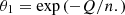
Nevertheless, we identified the least-damped baroclinic mode by scanning purely real eigenvalues and searching for an associated smooth (non-singular) eigenfunction. To facilitate numerical calculations, we imposed a mild density contrast between the top and bottom of the layer, setting Q = 1. In our reference 5 M⊙ model, η = 0.18. Using n = 3 and Et = 10−2, with Ω = 0.15 we find the least-damped baroclinic mode at λ=−8.33×10⁻³. Figure 4 illustrates the shape of this eigenmode, in which we include a small viscosity to reduce numerical noise. The temperature distribution closely resembles that of the Boussinesq case, while the velocity field is primarily concentrated within the tangent cylinder. This localisation imposes stronger shear in the velocity field; however, as the Prandtl number is small, this extra dissipation has little effect on the damping rate.
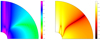 |
Fig. 4. Shape of the first baroclinic mode of a polytropic envelope, associated with eigenvalue λ=−8.33 10−3, for parameters η = 0.18, Ω = 0.15, Q = 1, n = 3, |

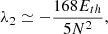
As shown in Fig. 5, this eigenvalue is proportional to Ω2 when Ω decreases to small values, as expected from the Boussinesq case. Moreover, it is not strongly affected by the density contrast of the layer. Figure 6 shows the variations with Q when the parameter is increased to realistic values (Q∼23), corresponding to our reference 5 M⊙ model. The figure shows that the dimensionless damping rate of this baroclinic mode is, for Q = 23, λ=−1.25×10⁻³, which differs little from the value at Q = 1, indicating a limited sensitivity to density contrast. We also verify that this eigenvalue is strictly proportional to Et, which characterises the heat diffusivity.
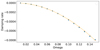 |
Fig. 5. Variation of the least-damped eigenvalue associated with the least-damped baroclinic mode as a function of rotation rate Ω for the anelastic model with Γ1 = 5/3, n = 3, Et = 10−3, η = 0.18, Q = 1, and |

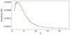 |
Fig. 6. Variation of the least-damped eigenvalue associated with the least-damped baroclinic mode as a function of the density contrast Q=ln(ρcore/ρsurf). Other parameters are as in Fig. 5, with Ω = 0.15. |
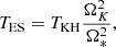
These results can be summarised by

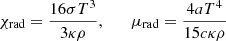
This expression is valid for low to moderate rotation rates, Ω≲0.5. With dimensional quantities, the timescale associated with this damping rate is
This expression indicates that the Kelvin-Helmholtz timescale is expected to be close to the thermal diffusion time across the convective core of the star, namely
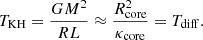
Figure 7 confirms this result by showing the ratio Tdiff/TKH as a function of the star mass for a series of models at ZAMS and terminal-age main sequence (TAMS).
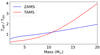 |
Fig. 7. Variation of the ratio between the thermal diffusion time over the core and the Kelvin-Helmholtz time at ZAMS and TAMS for masses of early-type stars. The thermal diffusion time is computed from Eq. (32). |
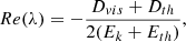
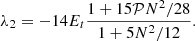
The damping time of the first baroclinic mode may now be compared to the Eddington-Sweet timescale, defined as
which is commonly used to estimate the timescale required for a rotating star to reach a steady state (Busse 1981; Zahn 1992). From Eq.(31), we find that
This result indicates that when the fractional radius of the stellar core is close to a tenth, the Eddington-Sweet timescale provides a good approximation of the damping timescale of baroclinic modes. Figure 8 shows tdamp/TES for ZAMS and TAMS models of early-type stars. At the ZAMS, the Eddington-Sweet timescale typically overestimates the damping timescale by a factor of four. In contrast, at the TAMS, the Eddington-Sweet timescale underestimates the damping time of baroclinic modes for masses above 10 M⊙. This reflects the effect of the small fractional radius of the stellar core at the TAMS, as suggested by (34).
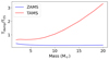 |
Fig. 8. Ratio of damping timescale to the Eddington-Sweet timescale at the ZAMS and TAMS for masses of early-type stars. |
4.3.2. The role of viscosity
These results are consistent with those from the Boussinesq model, once we admit that the key diffusivity controlling the damping rate of baroclinic modes is the one at the base of the radiative envelope. However, these findings are based on the assumption of a vanishing Prandtl number, i.e. a vanishing viscosity. We now examine this hypothesis.
At the microscopic level, radiative viscosity, given by photons, dominates over collisional viscosity due to the high temperatures inside early-type stars. Using
for the radiative conductivity and the radiative dynamic viscosity, respectively, we obtain the ‘radiative Prandtl number’.

which is essentially the squared ratio of the sound speed to the speed of light. In our 5 M⊙ reference model,  is always less than 10−4.
However, baroclinic-induced differential rotation is likely to generate small-scale turbulence in the radiative envelope of rotating stars (see Zahn 1992). This turbulence can carry momentum. Its action is commonly represented by horizontal and vertical viscosities3 (Zahn 1992). Moreover, gravito-inertial waves can also contribute to macroscopic transport, thus enhancing its efficiency (Mathis 2025). Hence, the actual effective Prandtl number could be much higher than 10−4.
As mentioned above, asteroseismology suggests diffusivities of D∼107 cm2/s for the momentum transport (Mombarg 2023), a value also adopted in the 2D-ESTER models of Mombarg et al. (2023). We adopt this value and impose a constant kinematic viscosity throughout the radiative envelope. As a result, the dynamic viscosity varies with the density, following θn in our model (see the momentum equation in Eq. (23)) and is therefore very small near the surface.
To illustrate the possible influence of viscosity, Fig. 9 shows three profiles of the Prandtl number for our 5 M⊙ reference model: (i) the classical radiative profile, for reference; (ii) the profile obtained with a constant kinematic viscosity at 107 cm2/s; and (iii) the profile from our polytropic envelope model with the same kinematic viscosity. This final profile reproduces the more realistic ESTER model quite faithfully.
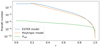 |
Fig. 9. Prandtl number profiles for a 5 M⊙ model. The blue line shows the ESTER model with a constant kinematic viscosity of ν = 107 cm2/s. The orange line represents the Prandtl number profile in the envelope based on the polytropic model described in Sect. 4.1.1. For comparison, the radiative Prandtl number, |

From Fig. 9, we see that the turbulent Prandtl number at the base of the radiative envelope is of order 10−1.
4.3.3. The eigenvalue spectrum
To proceed, we now investigate the eigenvalue spectrum, particularly the non-oscillating part, which lies on the real axis of the complex plane. Figure 10 (top) shows four series of eigenvalues computed with a small Prandtl number, that is,  . The red dots and the blue stars, which are superposed, were computed with identical parameters except that the heat diffusivity was increased by 2% for the blue symbols. In this case, most eigenvalues remain unchanged, except for two that shift to lower values (i.e. higher damping). These are the first two baroclinic modes, which are primarily damped by thermal diffusion. Other eigenvalues are associated with viscous modes, which are insensitive to heat diffusion. When the Prandtl number is kept fixed-by simultaneously increasing both viscosity and heat diffusivity-all eigenvalues scale with heat diffusivity. This behaviour is illustrated by the blue dots and the perfectly superposed black and white stars in Fig. 10 top. In a second test, shown in Fig. 10 (bottom), we considered a much higher Prandtl number, of the order of 0.1. The heat diffusivity was kept constant, while the viscosity was varied by 2%. As a result, the Prandtl number varied accordingly. We rescaled the eigenvalues computed with the new viscosity so that purely viscous eigenvalues would superpose. The figure shows that these are relatively few, essentially because the Prandtl number is much higher than in Fig. 10 (top) which increases the influence of viscosity.
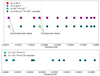 |
Fig. 10. Distribution of eigenvalues along the real axis. Top panel: Results for constant viscosity (top line) or constant Prandtl number (bottom line). Eigenvalues are computed with parameters n = 3, Q = 1, Ω = 0.15, η = 0.18, Lmax = 100, and Nr = 50 using the QZ-algorithm. Parameters E and Et are given in the legend. Bottom panel: Same as above, but with constant heat diffusion and varying viscosity. Eigenvalues have been rescaled by the ratio of viscosities. |
Finally, we traced the evolution of four eigenvalues near the first baroclinic mode (see Fig. 10, top) of the viscous problem as the rotation parameter, Ω, is varied. The result is shown in Fig. 11. This figure shows that as a parameter such as Ω is varied, many avoided crossings occur. In this case, the baroclinic eigenvalue (red dots in Ω = 0.175) decreases in absolute value as Ω2 and collides with viscous eigenvalues that are almost independent4 of Ω. Thus, unlike the case  discussed previously, the evolution of baroclinic eigenvalues with Ω is much more complex.
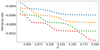 |
Fig. 11. Simultaneous evolution of four eigenvalues as a function of rotation. Parameters are as in Fig. 10, except E = 10−6 and Et = 10−3. At Ω = 0.15, the green dot indicates the first baroclinic eigenvalue shown in Fig. 10 (top). |
These results show that the influence of viscosity is not negligible for values ∼107 cm2/s. Tests on the dependence of the damping of baroclinic modes with respect to viscosity yield power laws λ∝Eα, with 0.2≲α≲0.5.
4.4. Discussion
The computation of baroclinic modes using a viscous polytropic model for the envelope of an early-type star shows that the key properties controlling the damping rates of non-oscillating modes are the fluid viscosity and heat diffusivity near the core-envelope interface. The results also show that the asymptotic case of a vanishing Prandtl number is an overly simplistic approximation. A non-zero Prandtl number allows for the existence of numerous purely viscous modes with a longer damping timescale.
Unlike the Boussinesq case, no general asymptotic law exists unless the angular velocity, density ratio Q, aspect ratio η, and Prandtl number are kept constant. In this case, the damping rates scale linearly with the viscosity and the spectrum is self-similar. Otherwise, the different dependence of each eigenvalue on these parameters leads to avoided crossings, which preclude the existence of any simple law.
With these results, we can now compare the damping rate of baroclinic modes, neglecting viscosity, to the nuclear timescale for models of various masses and ages. We define the nuclear timescale as the evolution of the average hydrogen mass fraction in the core (like in Gagnier et al. 2019). From (31), we find that the damping timescale is always less than one hundredth of the nuclear time, for all masses in the range 2 M⊙ to 20 M⊙. The damping of baroclinic modes cannot explain the transition in mass, around 7 M⊙, observed by Mombarg et al. (2024) (see the introduction). Therefore, a longer timescale must be considered, and our analysis of the eigenvalue spectrum suggests that viscous modes are better candidates. We computed the ratio of the viscous diffusion time, based on the half-radius of the star and the viscosity of the model (107 cm2/s) to the nuclear evolution time at the ZAMS and later. As shown in Fig. 12, this timescale appears to be the relevant one: only stars with masses less than 6 M⊙ have a viscous timescale short enough to follow the nuclear evolution. This figure also shows that this ratio (Tvisc/Tnuc) increases with time, and at mid-main sequence, even the 6 M⊙ model must lose the quasi-steady state, as the two timescales become comparable.
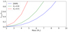 |
Fig. 12. Ratio of viscous time Tvisc=(R/2)2/ν* to the nuclear time, shown for various masses and three stages of evolution labelled by Xc=Xcore/Xenvelope. |
These results prompted us to perform a new simulation of a 2D time-dependent ESTER model as in Mombarg et al. (2024), but with a tenfold increase in viscosity (108 cm2/s). As shown in Fig. 13, even a 10 M⊙ model now relaxes to a quasi-steady state that allows it to reach critical rotation during the main sequence. At such high masses, angular momentum losses by winds are no longer negligible, as shown by Gagnier et al. (2019).
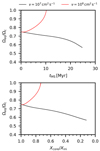 |
Fig. 13. Comparison of the evolution of two 10 M⊙ models with different kinematic viscosities, shown as a function of time spent on the main sequence (top panel) and as a function of the normalised hydrogen mass fraction in the core (bottom panel). |
For completeness, we also investigated the role of metallicity on the damping rate of eigenmodes, which may be summarised as a more efficient damping, as already observed by Mombarg et al. (2024). Details are provided in Appendix B.
5. Summary and conclusions
One of the main motivations for the present work was to understand the rotational evolution of two-dimensional ESTER models described in Mombarg et al. (2024). These models show the time evolution of fast rotating stars driven by nuclear reactions, including their centrifugal distortion and baroclinic flows (differential rotation and meridional circulation). A uniform kinematic viscosity of 107 cm2/s was imposed on the fluid, based on asteroseismic constraints and numerical stability. This modelling revealed the surprising result that, above a certain mass around 7 M⊙, models never reach critical rotation during the main sequence. Mombarg et al. (2024) explain this result by the difference between the nuclear timescale and the damping time of baroclinic modes, following the work of Busse (1981). However, Busse (1981) based his analysis on the very simple model of a plane horizontal fluid layer using the Boussinesq approximation in the asymptotic case of a vanishing Prandtl number. We therefore reconsidered this problem and extended it to a more realistic set-up.
As a first step, we extended Busse's analysis to spherical geometry, keeping both the Boussinesq approximation and the zero Prandtl number. We find the damping rates to be very close to those predicted with Busse's plane layer model. To extend the analysis, we replaced the Boussinesq approximation with the anelastic approximation, which allowed us to account for the large variations in the background density. Moreover, we included a finite Prandtl number because estimates of turbulent viscosity suggest that this parameter is not very small at the base of the radiative envelope. However, to maintain simplicity in the model, we restricted the computation to a spherical polytropic layer with an analytically describable density profile. We assumed a constant kinematic viscosity and a constant thermal conductivity. This model reproduces the strong variations of heat diffusivity in stars caused by density variations quite faithfully. With this model, we identified the classical Kelvin-Helmholtz time with the diffusion time over the convective core, provided the diffusivity was evaluated at the core-envelope interface. We also showed that the Eddington-Sweet timescale provides a realistic order of magnitude for the damping time of baroclinic modes. We then demonstrated that taking the limit of a vanishing Prandtl number oversimplifies the problem by eliminating all viscous modes. We showed that baroclinic modes interact increasingly with viscous modes as the Prandtl number increases. For the value used in Mombarg et al. (2024), viscous modes appear to play an essential role in the relaxation of the star towards a quasi-steady state. Considering viscously damped modes allowed us to interpret the mass limit, around 7 M⊙, beyond which 2D-ESTER models no longer reach critical rotation during the main sequence. A new simulation with a larger viscosity confirmed its crucial role in the rotational evolution of 2D-ESTER models: with a kinematic viscosity of 108 cm2/s, even a 10 M⊙ model can relax to a quasi-steady state during main sequence evolution and reach critical rotation (Fig. 13). We also investigated the role of metallicity and find that less metallic stars relax more quickly to the quasi-steady state. They are thus more prone to reaching critical rotation, which is in line with the results of Mombarg et al. (2024).
In conclusion, our work illustrates another consequence of angular momentum transport in stars: the ability of rotating early-type stars to reach critical rotation during the main sequence. If we assume that critical or near-critical rotation is associated with the well-known Be phenomenon (Porter & Rivinius 2003), this phenomenon may serve as a measure of angular momentum transport in radiative envelopes. However, before this can be assessed, we need to investigate how nuclear evolution excites viscous modes. This is the next step to improve our understanding of the dynamical evolution of rotating early-type stars.
Acknowledgments
We are very grateful to the referee for many valuable comments, which helped us improve the original manuscript. The research leading to these results has received funding from the French Agence Nationale de la Recherche (ANR), under grant MASSIF (ANR-21-CE31-0018-02) and from the European Research Council (ERC) under the Horizon Europe programme (Synergy Grant agreement N°101071505: 4D-STAR). While partially funded by the European Union, views and opinions expressed are however those of the authors only and do not necessarily reflect those of the European Union or the European Research Council. Neither the European Union nor the granting authority can be held responsible for them. MR also acknowledges support from the Centre National d’Etudes Spatiales (CNES). Computations of ESTER models and oscillation spectra have been possible thanks to HPC resources from CALMIP supercomputing centre (Grant 2025-P0107).
This follows from the heat flux equation, 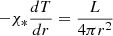 , and the hydrostatic equation (17).
At first sight, this may be surprising because we expect Ekman layers at the boundaries of the domain. However, because of the stress-free boundary conditions used in our model, viscous dissipation remains weakly dependent on Ω (e.g. Rieutord & Zahn 1997).
References
- Busse, F. 1981, Geophys. Astrophys. Fluid Dyn., 17, 215 [Google Scholar]
- Busse, F. 1982, ApJ, 259, 759 [Google Scholar]
- Chandrasekhar, S. 1961, Hydrodynamic and Hydromagnetic Stability (Oxford: Clarendon Press) [Google Scholar]
- Dintrans, B., & Rieutord, M. 2001, MNRAS, 324, 635 [Google Scholar]
- Dintrans, B., Rieutord, M., & Valdettaro, L. 1999, J. Fluid Mech., 398, 271 [Google Scholar]
- Eddington, A. S. 1925, The Observatory, 48, 73 [NASA ADS] [Google Scholar]
- Ekström, S., Meynet, G., Maeder, A., & Barblan, F. 2008, A&A, 478, 467 [Google Scholar]
- Espinosa Lara, F., & Rieutord, M. 2011, A&A, 533, A43 [NASA ADS] [CrossRef] [EDP Sciences] [Google Scholar]
- Espinosa Lara, F., & Rieutord, M. 2013, A&A, 552, A35 [NASA ADS] [CrossRef] [EDP Sciences] [Google Scholar]
- Fornberg, B. 1998, A Practical Guide to Pseudospectral Methods (Cambridge University Press) [Google Scholar]
- Gagnier, D., & Rieutord, M. 2020, J. Fluid Mech., 904, A35 [NASA ADS] [CrossRef] [Google Scholar]
- Gagnier, D., Rieutord, M., Charbonnel, C., Putigny, B., & Espinosa Lara, F. 2019, A&A, 625, A89 [NASA ADS] [CrossRef] [EDP Sciences] [Google Scholar]
- Granada, A., Ekström, S., Georgy, C., et al. 2013, A&A, 553, A25 [NASA ADS] [CrossRef] [EDP Sciences] [Google Scholar]
- Hastings, B., Wang, C., & Langer, N. 2020, A&A, 633, A165 [NASA ADS] [CrossRef] [EDP Sciences] [Google Scholar]
- Iqbal, S., & Keller, S. C. 2013, MNRAS, 435, 3103 [NASA ADS] [CrossRef] [Google Scholar]
- Kippenhahn, R., & Weigert, A. 1990, Stellar Structure and Evolution (Springer) [Google Scholar]
- Martayan, C., Baade, D., & Fabregat, J. 2010, A&A, 509, A11 [NASA ADS] [CrossRef] [EDP Sciences] [Google Scholar]
- Mathis, S. 2025, A&A, 694, A173 [NASA ADS] [CrossRef] [EDP Sciences] [Google Scholar]
- Mombarg, J. S. G. 2023, A&A, 677, A63 [NASA ADS] [CrossRef] [EDP Sciences] [Google Scholar]
- Mombarg, J. S. G., Rieutord, M., & Espinosa Lara, F. 2023, A&A, 677, L5 [NASA ADS] [CrossRef] [EDP Sciences] [Google Scholar]
- Mombarg, J. S. G., Rieutord, M., & Espinosa Lara, F. 2024, A&A, 683, A94 [NASA ADS] [CrossRef] [EDP Sciences] [Google Scholar]
- Porter, J. M., & Rivinius, T. 2003, PASP, 115, 1153 [Google Scholar]
- Reese, D., Lignières, F., & Rieutord, M. 2006, A&A, 455, 621 [NASA ADS] [CrossRef] [EDP Sciences] [Google Scholar]
- Rieutord, M. 2006, in Stellar Fluid dynamics and numerical simulations: From the Sun to Neutron Stars, eds. M. Rieutord, & B. Dubrulle, EAS Pub., 21, 275 [Google Scholar]
- Rieutord, M., & Zahn, J. -P. 1997, ApJ, 474, 760 [Google Scholar]
- Rieutord, M., Espinosa Lara, F., & Putigny, B. 2016, J. Comp. Phys., 318, 277 [NASA ADS] [CrossRef] [Google Scholar]
- Schootemeijer, A., Lennon, D. J., Garcia, M., et al. 2022, A&A, 667, A100 [NASA ADS] [CrossRef] [EDP Sciences] [Google Scholar]
- Stewartson, K. 1966, J. Fluid Mech., 26, 131 [NASA ADS] [CrossRef] [Google Scholar]
- Sweet, P. A. 1950, MNRAS, 110, 548 [Google Scholar]
- von Zeipel, H. 1924, MNRAS, 84, 665 [NASA ADS] [CrossRef] [Google Scholar]
- Zahn, J. -P. 1992, A&A, 265, 115 [Google Scholar]
Appendix A: Projection of the equations of motion onto spherical harmonics
In order to solve numerically system (23), we use a spectral method projecting the unkown on spherical harmonics and then discretizing the radial dependence on the Gauss-Lobatto grid associated with Chebyshev polynomials.
To ease the resolution we first introduce the function
then expanding the viscous force as
the radial functions read
where Λ=ℓ(ℓ+1). Indices (ℓ,m) have been omitted for radial functions  to simplify notations. Primes are for derivatives.
It is also useful to introduce dependent variables π and b such that p=θnπ and ρ=θn−1b as suggested by Reese et al. (2006), hence
from the perturbed equation of state of the ideal gas. After some tedious manipulations, where we elminate bℓ and vℓ, we find the following equations:
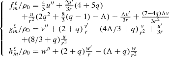
![$$ \begin{aligned}&&\lambda {u_\ell }+ 2\Omega \left ((\ell -1)\alpha _{\ell -1}w^{\ell -1}- (\ell +2)\alpha _{\ell +1}w^{\ell +1}\right )\\ &&\qquad = -\pi '_\ell - \left (\frac {q}{r} + \frac {(n+1)B}{r^2\theta }\right )\pi _\ell +\frac {{t^\ell _m}}{r^2\theta } \\ && \qquad \qquad +E \left [u''_\ell + {\cal {{A}}}_1\frac {u'_\ell }{3r} + {\cal {{A}}}_2\frac {u_\ell }{3r^2} \right ]\end{aligned} $$](/articles/aa/full_html/2025/07/aa55003-25/aa55003-25-eq80.gif)
with  and
and  defined as

![$$ \begin{aligned}&&\lambda (ru'_\ell +(2+q)u_\ell ) + 2\Omega \left (B_{\ell -1}w^{\ell -1}+B_{\ell +1}w^{\ell +1}\right )\\ && =-\frac {\Lambda \pi _\ell }{r}+ E \left [ru'''_\ell + {\cal {{B}}}_1u''_\ell + {\cal {{B}}}_2\frac {u'_\ell }{r} + {\cal {{B}}}_3\frac {u_\ell }{r^2} \right ]\end{aligned} $$](/articles/aa/full_html/2025/07/aa55003-25/aa55003-25-eq84.gif)
with ℬ1, ℬ2 and ℬ3 defined as
![$$ \begin{aligned}&& \lambda {w_\ell }-2\Omega \left [A_{\ell -1}\left (ru'_{\ell -1}+ \mbox {${{\cal {{C}}}}$}_1{u^{\ell -1}} \right )+A_{\ell +1}\left (ru'_{\ell +1}+ \mbox {${{\cal {{C}}}}$}_2{u^{\ell +1}} \right )\right ]\\ && \qquad = E\left [w''_\ell +(2+q)\frac {w'_\ell }{r}-(\Lambda +q)\frac {w_\ell }{r^2} \right ]\end{aligned} $$](/articles/aa/full_html/2025/07/aa55003-25/aa55003-25-eq86.gif)
with  and
and  defined as

The energy equation now reads
![$$ \lambda \left [G_1\pi _\ell +\Gamma _1{t_\ell }\right ]+ N_1\theta '{u^\ell _m}= \frac {E_T}{\theta ^n}\Delta _\ell {t^\ell _m} $$](/articles/aa/full_html/2025/07/aa55003-25/aa55003-25-eq90.gif)
with

and B given by (24).
Appendix B: Role of metallicity
Metallicity has only a mild impact on the damping rates: when metallicity is reduced from Z = 0.02 to Z = 0.001, baroclinic modes show a damping rate increased by ∼25%, while viscous modes show a stronger effect with a damping rate increased by ∼50%. We illustrate this trend in Fig. B.1. It is coherent with what Mombarg et al. (2024) observed, namely that less metallic models reach criticality more easily, and is inline with observations, which reveal that Be stars are more common in galaxies of low metallicity like the SMC (Martayan et al. 2010; Iqbal & Keller 2013; Schootemeijer et al. 2022). Qualitatively, low metallicity stars are of smaller size, which shortens all diffusion times.
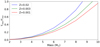 |
Fig. B.1. Ratio of viscous time Tvisc=(R/2)2/ν* to the nuclear time as a function of mass for ZAMS models at three different metallicities. |
All Figures
|
Fig. 1. Meridional view of the least-damped baroclinic mode. Left: streamlines of the meridional velocity; middle: azimuthal velocity; right: temperature perturbation. In the middle and right panels, solid lines indicate the change of sign of the field. The solution is associated with the eigenvalue λ=−8.653×10⁻³ obtained with parameters E = 0, Et = 10−3, N = 1, and numerical resolution Lmax = 50, Nr = 50. |
| In the text | |
|
Fig. 2. Damping rate of the least-damped baroclinic mode in the spherical Boussinesq model as a function of the ratio N=N*/2Ω*, for |
| In the text | |
|
Fig. 3. Radial profiles of the thermal conductivity (left), thermal diffusivity (middle), and the resulting non-dimensional parameter Et (right) for a non-rotating 5 M⊙ ESTER model at the zero-age main sequence (ZAMS). |
| In the text | |
|
Fig. 4. Shape of the first baroclinic mode of a polytropic envelope, associated with eigenvalue λ=−8.33 10−3, for parameters η = 0.18, Ω = 0.15, Q = 1, n = 3, |
| In the text | |
|
Fig. 5. Variation of the least-damped eigenvalue associated with the least-damped baroclinic mode as a function of rotation rate Ω for the anelastic model with Γ1 = 5/3, n = 3, Et = 10−3, η = 0.18, Q = 1, and |
| In the text | |
|
Fig. 6. Variation of the least-damped eigenvalue associated with the least-damped baroclinic mode as a function of the density contrast Q=ln(ρcore/ρsurf). Other parameters are as in Fig. 5, with Ω = 0.15. |
| In the text | |
|
Fig. 7. Variation of the ratio between the thermal diffusion time over the core and the Kelvin-Helmholtz time at ZAMS and TAMS for masses of early-type stars. The thermal diffusion time is computed from Eq. (32). |
| In the text | |
|
Fig. 8. Ratio of damping timescale to the Eddington-Sweet timescale at the ZAMS and TAMS for masses of early-type stars. |
| In the text | |
|
Fig. 9. Prandtl number profiles for a 5 M⊙ model. The blue line shows the ESTER model with a constant kinematic viscosity of ν = 107 cm2/s. The orange line represents the Prandtl number profile in the envelope based on the polytropic model described in Sect. 4.1.1. For comparison, the radiative Prandtl number, |
| In the text | |
|
Fig. 10. Distribution of eigenvalues along the real axis. Top panel: Results for constant viscosity (top line) or constant Prandtl number (bottom line). Eigenvalues are computed with parameters n = 3, Q = 1, Ω = 0.15, η = 0.18, Lmax = 100, and Nr = 50 using the QZ-algorithm. Parameters E and Et are given in the legend. Bottom panel: Same as above, but with constant heat diffusion and varying viscosity. Eigenvalues have been rescaled by the ratio of viscosities. |
| In the text | |
|
Fig. 11. Simultaneous evolution of four eigenvalues as a function of rotation. Parameters are as in Fig. 10, except E = 10−6 and Et = 10−3. At Ω = 0.15, the green dot indicates the first baroclinic eigenvalue shown in Fig. 10 (top). |
| In the text | |
|
Fig. 12. Ratio of viscous time Tvisc=(R/2)2/ν* to the nuclear time, shown for various masses and three stages of evolution labelled by Xc=Xcore/Xenvelope. |
| In the text | |
|
Fig. 13. Comparison of the evolution of two 10 M⊙ models with different kinematic viscosities, shown as a function of time spent on the main sequence (top panel) and as a function of the normalised hydrogen mass fraction in the core (bottom panel). |
| In the text | |
|
Fig. B.1. Ratio of viscous time Tvisc=(R/2)2/ν* to the nuclear time as a function of mass for ZAMS models at three different metallicities. |
| In the text | |
Current usage metrics show cumulative count of Article Views (full-text article views including HTML views, PDF and ePub downloads, according to the available data) and Abstracts Views on Vision4Press platform.
Data correspond to usage on the plateform after 2015. The current usage metrics is available 48-96 hours after online publication and is updated daily on week days.
Initial download of the metrics may take a while.