| Issue |
A&A
Volume 699, July 2025
|
|
|---|---|---|
| Article Number | L7 | |
| Number of page(s) | 6 | |
| Section | Letters to the Editor | |
| DOI | https://doi.org/10.1051/0004-6361/202554974 | |
| Published online | 09 July 2025 | |
Letter to the Editor
Magnetospheric magnetic reconnection in high-mass young stellar objects and its possible relation to methanol maser flares
1
Mathematics and Mechanics Faculty, Saint-Petersburg State University, Saint-Petersburg 198504, Russia
2
Ural Federal University, Ekaterinburg 620000, Russia
3
Xinjiang Astronomical Observatory, Chinese Academy of Sciences, Urumqi 830011, China
4
Center for Astrophysics, Guangzhou University, Guangzhou 510006, China
5
Shanghai Astronomical Observatory, Chinese Academy of Sciences, 80 Nandan Road, Shanghai 200030, China
⋆ Corresponding author: s.khaibrakhmanov@gmail.com
Received:
1
April
2025
Accepted:
14
June
2025
Context. Maser emission is an inherent property of regions of high-mass star formation. Often the masers exhibit flares with duration times from several hours to tens of years. The nature of long-time flares can be explained by the model of episodic accretion. The origin of short-time flares is still uncertain.
Aims. Our goal is to elaborate on the physics of short-time maser flares in the region of high-mass star formation G33.641-0.228.
Methods. Based on an analysis of the observational data and predictions of the star formation theory, we hypothesise that the young star in G33.641-0.228 has a magnetosphere and is surrounded by the circumstellar disc threaded by a large-scale magnetic field. We use the equations of the standard accretion disc theory to analyse the interaction of the accretion flow with the magnetosphere. We propose that the boundary of the magnetosphere is a current sheet and analyse possible magnetic reconnection speeds, as well as estimate the corresponding amount and timescales of magnetic energy release.
Results. Our estimates show that the magnetospheric current sheet can exist in two states. In a quiescent state, the magnetic reconnection is slow, and the magnetic energy release is small. In a burst state, interchange and other magneto-hydrodynamic (MHD) instabilities cause turbulence generation in the flow. The magnetic reconnection switches to a fast regime driven by turbulence, and the energy release becomes significant compared to the luminosity of a protostar. The time of fast magnetic reconnection is ≲1 day, which is comparable to observed rise times of maser flares in G33.641-0.228.
Conclusions. Magnetic reconnection of stellar and disc magnetic fields near the magnetosphere can be a mechanism for short-time maser flares in G33.641-0.228 and similar objects. This process can be accompanied by X-ray flares; therefore, coordinated high-angular and high-time observations of maser flares, IR, and X-ray emission represent a promising new way of studying high-mass star formation.
Key words: accretion, accretion disks / magnetic reconnection / masers / stars: massive / stars: protostars / ISM: magnetic fields
© The Authors 2025
 Open Access article, published by EDP Sciences, under the terms of the Creative Commons Attribution License (https://creativecommons.org/licenses/by/4.0), which permits unrestricted use, distribution, and reproduction in any medium, provided the original work is properly cited.
This article is published in open access under the Subscribe to Open model. Subscribe to A&A to support open access publication.
1. Introduction
Maser emission is one of the remarkable features of star formation in the interstellar medium. In particular, class II methanol masers (cIIMMs) pumped by radiation are associated with the physical processes in high-mass star formation regions (HMSFRs, e.g. Paulson & Pandian 2020). It has been found that cIIMMs arise in the surface layers of protostellar discs surrounding massive young stellar objects (MYSOs), as well as in the outflows from MYSOs (Moscadelli et al. 2024). The study of masers is useful for estimations of the gas physical state. For example, cIIMMs trace spiral arms in the protostellar discs (Chen et al. 2020). Maser transitions are prone to the Zeeman effect, which is used to estimate magnetic field strength in the masing region. Magnetic field measurements via detection of the Zeeman effect together with polarisation maps of surrounding gas (Dall’Olio et al. 2019) indicate that the magnetic field is an essential component of HMSFRs (Vlemmings 2008; Lankhaar et al. 2018).
The emission from MYSOs exhibits time variability in different spectral ranges (Fischer et al. 2023). The study of such phenomena requires coordinated follow-up observations (Burns 2024). In many cases, the maser variability appears in the form of separate flares, during which the flux rises by several orders of magnitude. The durations of the flares range from several days to tens of years. An interesting group of maser sources in HMSFRs comprises objects with irregular maser flares characterised by short duration times of several days or months (Szymczak et al. 2018). A characteristic example is G33.641-0.228, where several flares have been observed since 2009 (Fujisawa et al. 2012, 2014; Aberfelds et al. 2023). A remarkable feature of this object is small-amplitude flux variations during the flares.
Methanol maser variability could be related to spiral shocks in the circumstellar disc (Parfenov & Sobolev 2014), or it could be a consequence of the luminosity bursts in YSOs caused by episodic accretion of massive clumps from the disc (Meyer et al. 2017), hydrodynamic and magneto-hydrodynamic (MHD) instabilities in the disc (e.g. Vorobyov et al. 2020), or instabilities at the boundary between the disc and the star (Romanova et al. 2008). Each mechanism is characterised by a specific timescale. Clump accretion in massive YSOs leads to bursts with typical durations of more than 1 year (Elbakyan et al. 2021). This scenario was confirmed by the observations of IR bursts accompanying maser flares in several objects (Caratti o Garatti 2017; Stecklum et al. 2021). The irregular variability on timescales of days to months is less studied.
In this paper, we analyse the short-term maser flares in the region G33.641-0.228. We compile observational data on the maser flares in this object, analyse its properties, and use observational data to formulate a hypothesis about the MHD origin of the flares. We propose that the protostar has a magnetosphere, which interacts with the circumstellar accretion disc in a non-stationary way. We explore the possibility that the energy release in the current sheet (CS) formed at the magnetosphere boundary could be a source of luminosity bursts and corresponding maser flares.
2. Analysis of the observational data
2.1. G33.641-0.228 – prototypical example
Let us outline properties of masers in G33.641-0.228 (G33, hereafter). The distance to the G33 is 4 kpc and its bolometric luminosity, L⋆, is 1.2 ⋅ 104 L⊙, according to the IRAS database. The systematic radial velocity of the object is 60 km/s (Aberfelds et al. 2023). Six methanol maser components have been found in G33 (Szymczak et al. 2000). Bartkiewicz et al. (2009) and Fujisawa et al. (2012) have shown that the methanol maser spots form an ‘arch’ with a linear size of 650 au. A group of water masers has also been detected in G33. Bartkiewicz et al. (2012) made high-angular and high-spectral-resolution studies of G33 using the European VLBI Network and concluded that the methanol masers trace a circumstellar disc around the HMYSO, while the water masers originate in the outflows from the central source. Vlemmings (2008) detected the Zeeman splitting in the observed methanol maser components and deduced an estimate of the flux-averaged magnetic field strength in the region of masing gas, BM = 18 mG, which was stable across all components.
Fujisawa et al. (2012) used the Yamaguchi 32-m radio telescope to observe the masers within a period of 108 days in 2009. During this period, the flux density of components I and III-VI had a nearly constant flux. Component II (vLSR = 59.6 km/s) exhibited two large flares and one small flare. Between the flares, component II had a flux of 20 − 30 Jy comparable to components V and VI. During the two large flares, the flux density increased seven times above the quiescent state over 1 − 3 days and then decreased to the initial state over 5 days. Fujisawa et al. (2014) detected five more flares in component II in the period from 2009 to 2012. Each flare was characterised by an increase in the radiation flux density by 4 − 25 times (by ≈150 − 450 Jy) above the quiescent state over 1 − 3 days and a subsequent decrease in the flux density over 5 days. Kojima et al. (2018) detected 11 similar flares during the period from 2014 to 2015. Bērziṇš et al. (2018) reported a powerful outburst in component II, which occurred on August 25, 2016. The flux density increased 13-fold from 26 to 343 Jy during the maser flare. The fading phase of the outburst lasted about 25 days. The fact that the decay time of the flares is longer than the rise time is a common feature of many periodic maser sources (see Olech et al. 2019; Aberfelds et al. 2023).
The light curves from Fujisawa et al. (2012, 2014) demonstrate small amplitude oscillations in the fading phase of the flares in component II. The oscillation period is 1 − 2 days; the amplitude is ∼20 Jy. Kojima et al. (2018) detected similar fluctuations with a period of 5–6 hours. Bērziṇš et al. (2018) also recorded flux fluctuations with a period of several hours during the flare on August 25, 2016. Aberfelds et al. (2023) reported two additional bursts in component IV in 2018 and 2021, during which the flux density increased from 10 to 100 Jy and faded in ∼100 days. The second burst (2021) in component IV also exhibited flux fluctuations during the fading phase.
2.2. Properties of the masing gas in G33
It is believed that cIIMMs arise in the circumstellar discs of MYSOs (Norris et al. 1998). In such a case, the masing gas is located in the surface layers of the disc, and background radiation heating dust and pumping the maser comes from a central young star. In the following, we analyse the bursting behaviour of HMYSOs in G33 in the frame of the disc accretion scenario. Disc model equations are presented in Appendix A.
We propose that the temperature in a region of masing gas, Teff, is determined by the gas due to heating by the radiation of the star (see Appendix A). The characteristic temperature, TM, of the gas in the region of masing gas is of 100 − 120 K (Cragg et al. 2005). The corresponding density is nM = 106 cm−3. Assuming that TM ≈ Teff(rm) and using Eq. (A.10), one gets the distance between the central star in G33 and the region of masing gas: rM = 380 au. This distance is nearly half of the maximum distance between maser spots, 650 au, reported by Fujisawa et al. (2012). A value of rM ∼ 400 au can be considered as a radius of a ring-like region in the disc, where masers are induced. The maps of the masers’ distribution from Bartkiewicz et al. (2012) show that bursting component II lies approximately near the intersection of the methanol maser ‘arch’ and a ‘line’ connecting water masers. Outflows are predicted to originate in central regions of circumstellar discs (see Frank et al. 2014). It is reasonable, then, to propose that component II lies along the line of sight between the observer and the central star. We believe that component II should be considered not as a physical gas parcel (‘cloudlet’) orbiting a star, but as a spatial region along the line of sight, where the maser is pumped by the variable stellar radiation flux.
3. MHD scenario of the luminosity bursts
The detection of the magnetic field in G33 allows us to propose that the protostar formed in the medium threaded by a magnetic field. This assumption is consistent with the theory of star formation (McKee & Ostriker 2007). The theory indicates that the magnetic flux of molecular clouds is partially conserved during star formation, and YSOs are born having a large-scale ‘fossil’ magnetic field (Dudorov & Khaibrakhmanov 2015). The star, generally speaking, is formed surrounded by a magnetosphere.
The magnetic field of stars manifests itself in many observable phenomena, such as magnetically driven flares and related quasi-periodic oscillations (QPOs). The most studied example is the phenomenon of solar flares (Zimovets et al. 2021). Similar processes have already been observed in pre-main-sequence stars (Flaccomio et al. 2018; Jackman et al. 2019), where flares are detected both in the infrared and X-rays (Ke et al. 2012; Flaherty et al. 2014). Powerful flares around Sgr A* in the centre of the Galaxy are also explained by MHD processes in the accretion disc surrounding the black hole (Dexter et al. 2010; Porth et al. 2021). Energetic MHD processes are used to interpret flares observed in magnetars (Proga & Zhang 2006; Castro-Tirado et al. 2021) as well as the phenomenon of micro-quasars (de Gouveia Dal Pino & Lazarian 2005). Finally, MHD simulations of the accretion in low-mass YSOs indicate that the interaction of the disc’s magnetic field with a young star may lead to variability (Romanova & Kulkarni 2009; Takasao et al. 2019).
The key process responsible for impulsive energy release in all the above-mentioned models is the magnetic reconnection in the CSs formed in the regions of strong magnetic fields with opposite directions. The reconnection can take place either in the region of the interaction of the accretion flow with the stellar magnetosphere, or at the stellar surface. Based on the above considerations, we hypothesise that the short-term maser flares observed in G33 may be caused by corresponding emission flares near the stellar magnetosphere, where violent magnetic reconnection events take place episodically.
3.1. Analysis of the magnetic fields
Theoretical models predict that the surface magnetic field of a newly born star with mass M = 10 M⊙ may be of 1 − 200 Gs depending on the properties of ionising sources in the parent molecular cloud (Dudorov & Khaibrakhmanov 2015). Observational constraints on the magnetic field strength in young high-mass stars come from studies of Herbig Ae/Be stars (HAeBeSs) and OB stars. The HAeBeSs can have a surface magnetic field strength up to ∼400 G (Kholtygin et al. 2019). Measured surface magnetic fields in massive OB stars, M > 8 M⊙, range from 50 − 100 G to 1 − 16 kG (Hubrig et al. 2011; Grunhut et al. 2017).
We analysed the properties of the young high-mass star in G33, considering that it is the progenitor of an OB star. We adopted the following values of mass, effective temperature, and surface magnetic field strength as fiducial ones: T⋆ = 2 ⋅ 104 K, M⋆ = 10 M⊙, and Bsurf = 103 G, respectively. The corresponding fiducial radius of the star is 9.12 R⊙, which was calculated for a spherical black body with effective temperature T⋆ and luminosity of L⋆ = 1.2 ⋅ 104 L⊙. The rate of mass accretion onto the star, Ṁ, may lie in the range from ∼10−5 to 10−3 M⊙ yr −1 (Beltrán & de Wit 2016). We adopted Ṁ = 10−5 M⊙ yr −1 as a fiducial value and estimated the radius of the stellar magnetosphere from the balance of viscous and magnetic stresses (see Eq. (B.3)),
Such a small Rmag reflects strong ‘squeezing’ of the stellar magnetic configuration by the accretion flow with a high mass accretion rate. The case with a sufficiently high accretion rate and/or weak stellar magnetic field may lead to the state characterised by Rmag ≤ R⋆. Two accretion scenarios are possible, generally speaking. The first one, Rmag > R⋆, is the classical magnetospheric accretion that has been well studied for low-mass stars (see Hartmann et al. 2016). The second one, Rmag ≤ R⋆, corresponds to disc accretion directly onto the stellar surface. Equation (1) shows that the stars with 10−5 M⊙ yr −1 would have a magnetosphere if B⋆ ≳ 600 Gs. For the case Ṁ = 10−4 M⊙ yr −1 a magnetosphere exists if B⋆ > 2 kG, and for the case Ṁ = 10−3 M⊙ yr −1 the condition is B⋆ > 6 kG.
Equations (1)–(B.2) give the dipole magnetic field of the star:
The corresponding value of the disc’s magnetic field strength can be estimated considering that the disc is in magnetostatic equilibrium. Equation (A.11) from Appendix A gives:
A comparison of (2) and (3) shows that, given the parameters’ uncertainties, the stellar and disc magnetic fields are of the same order. According to the theory of the fossil magnetic field (Dudorov & Khaibrakhmanov 2015), it is natural to assume that these fields are in opposite directions, at least until the stellar dynamo sets in. Therefore, the region between the magnetosphere and the disc is a CS.
3.2. Quiescent state – slow magnetic reconnection
Since the boundary between the magnetosphere of a star and the disc is a CS, magnetic reconnection is expected to occur in this region. The rate of magnetic energy release in the CS is
where HCS is the height of the CS in the direction, z, perpendicular to the disc, and vin is the reconnection velocity.
In the classical Sweet-Parker model, the reconnection velocity is determined as  , where S = LvA/η is the Lundquist number, L is the CS length,
  is the Alfvén speed in the accretion flow, and η is the magnetic diffusivity (see Kadowaki et al. 2018).We define HCS as the curvature radius of the magnetosphere, HCL ≈ Rmag/3. If we assume that the magnetic flux dissipates inside the CS due to Ohmic dissipation, then η = c2/4πσ, where σ is the Coulomb conductivity. The plasma near the magnetosphere can have a temperature of 104 K, and therefore be considered to be fully ionised, and then σ = 107 T3/2 s−1 (e.g. Parker 1979) and
which means that the reconnection is very slow,  . The corresponding magnetic energy release is also very small, dEm/dt = 3.1 ⋅ 10−3 L⊙, under the parameters adopted.
3.3. Burst state – fast magnetic reconnection
Magnetospheric accretion is expected to be a non-steady phenomenon, since the interaction of the accretion flow with the stellar magnetic field is prone to an interchange instability (see Parker 1979) at the boundary of the magnetosphere (Romanova et al. 2008). The interchange instability develops if ρg⋆ > kB⋆2/4π, where g⋆ is the stellar gravity acceleration and k is the wavenumber of the magnetosphere boundary perturbation. This condition can be rewritten in the form n > ncrit, where the critical value of the gas number density, ncr, corresponds to a transition state between stability and instability. The wavenumber, k, can be estimated to be equal to 1/Rc, where Rc ≈ Rmag/3 is the curvature of the magnetic field lines. In the case of disc accretion onto the magnetosphere of radius (1), the instability criterion leads to

A comparison of Eq. (6) and Eq. (A.8) shows that the magnetosphere boundary is unstable for the fiducial parameters adopted.
The inner part of the disc is probably turbulent due to the magneto-rotational (MRI) and Parker-Rayleigh-Taylor (PRT) instabilities, as is indicated by numerical simulations (e.g. Kadowaki et al. 2018). Then the CS at the boundary of the magnetosphere is embedded in the turbulent medium from both sides.
In the case of turbulent mixing of plasma, the magnetic reconnection in the CS switches to a fast regime (Lazarian & Vishniac 1999). The reconnection rate can reach a significant fraction of the Alfvén speed,  , where the reconnection rate is f = 0.05 − 0.2 (Kowal et al. 2009; Kadowaki et al. 2018). Most of the reconnection takes place in the corona above the disc. The strength of the large-scale poloidal magnetic field can be considered to be nearly constant with height, according to the condition div B = 0. On the contrary, the gas density decreases according to the hydrostatic solution (A.3). Then one gets ρ(z)≈0.01ρ(z = 0) for z = HCS and typical H/Rmag = 0.1. Using Eqs. (3) and (A.8) to estimate the Alfvén speed in the CS, we obtain the final estimate from (4)

That is, the ‘luminosity’ of the CS in the region of fast magnetic reconnection is up to 5 − 6% of the total bolometric luminosity of the HMYSO. This estimate allows us to suppose that maser flares in HMYSO may be related to the luminosity bursts caused by the magnetic reconnection near the stellar magnetosphere.
Let us estimate the timescale of the magnetic reconnection, which determines the characteristic rise time of the flare in the proposed scenario. The reconnection time can be defined as trec ≈ Rmag/vrec (see Shibata & Magara 2011); then
The reconnection time is of ≲1 day, which is close to maser flare rise times found for G33.
A sufficiently thin CS is subject to the tearing instability, which leads to the cascade magnetic reconnection (Shibata & Tanuma 2001). This process develops in a non-turbulent regime and is characterised by smaller reconnection speeds of  that are variable in time (see Bhattacharjee et al. 2009). The cascade leads to the formation of small plasma blobs or eddies inside the CS. We suppose that the tearing-mode-driven reconnection may occur in a quiescent state before a main flare, when the magnetosphere boundary is non-turbulent. The heating caused by such a process may potentially be a reason for the small-amplitude maser flux variations during the growth phase of large flares in G33. In turn, post-flare flux variations can be caused by the final stages of decaying turbulence in the CS, since this process is characterised by energy exchange between compressible and incompressible MHD waves (see Mac Low et al. 1998; Cho & Lazarian 2002; Suzuki et al. 2007).
4. Conclusions and discussion
We analysed the variability of methanol masers in the HMSFR G33. Based on the analysis of the methanol and water maser spots’ distribution, we treated G33 as a system consisting of a young high-mass star surrounded by a circumstellar accretion disc seen nearly edge-on. Our estimates show that the radius of the disc, out of which the maser emission comes, is 400 au.
We state that the flaring component II of G33 is situated along the line of sight. The flux variations in component II are related, then, to the variations in the radiation flux coming from the star. The episodic accretion model cannot explain the short-time flares in G33 having a duration in the range from a few days to 2–3 months. We propose an alternative scenario based on the model of magnetospheric accretion.
The predictions of the star formation theory and measurements of the magnetic field in G33 allow us to propose that the HMYSO has a magnetic field of a fossil nature. We show that the star may have a magnetosphere with a radius of 1.1 R⋆ for typical parameters of a young O star that is accreting at a rate of 10−5 M⊙ yr−1 and that has a surface magnetic field of 1 kG. The magnetic field strength is 750 G at the boundary of the magnetosphere, for fiducial parameters of the model. We used the power law dependence of the magnetic field strength on gas density in the magnetostatic disc, Bdisk ∝ ρ1/2, to estimate the disc’s magnetic field strength at the magnetosphere boundary, 1880 G. The approximate equality of the stellar and disc’s magnetic fields means that the magnetosphere boundary is a CS. We hypothesise that the magnetic energy liberated in a process of magnetic reconnection inside this CS contributes to the overall luminosity of the HMYSO and, correspondingly, influences the maser emission. A similar idea was stated by Fujisawa et al. (2012), though the authors speculated that the reconnection takes place in the disc near the region of maser formation.
We propose that the magnetospheric accretion in G33 switches between two states (see Fig. 1). In a quiescent state, the magnetosphere boundary is stable and the magnetic reconnection is slow. In this state, the magnetic energy released in the CS is much smaller than the bolometric luminosity of the HMYSO. In the burst state, the magnetosphere becomes unstable to interchange, MRI, and PRT instabilities on both sides of the CS. The instabilities lead to the turbulence generation in the flow near the magnetosphere and increase the magnetic reconnection rate. An analytical model for magnetic reconnection near the magnetospheres of YSOs has been presented by de Gouveia Dal Pino et al. (2010). A similar process has been numerically studied in application to flares in Sgr A* (e.g. Rodríguez-Ramírez et al. 2019). Compared to the quiescent state, the magnetic power released is larger and equals ≈830 L⊙ for the parameters adopted, which is 5 − 6% of the total bolometric luminosity of the MYSO. Therefore, the fast magnetic reconnection events can lead to the luminosity bursts and, as a consequence, cause the maser flares. We show that the reconnection timescale is ≲1 day for typical parameters, which is comparable with the rise time of methanol flares in G33. After the energy release, the flow near the magnetosphere becomes stable, and the system switches to a quiescent state until a sufficient mass and magnetic flux is accumulated near the magnetosphere again. We propose that the small-amplitude flux variations during maser flares can be caused by variable-in-time magnetic reconnection driven by the tearing mode instability before the flare and decaying turbulence after the flare.
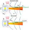 |
Fig. 1. Schematic picture of the maser flaring scenario. The quiescent state is characterised by slow magnetic reconnection in the CS at the magnetosphere’s boundary. The corresponding maser flux is F. In the burst state, fast magnetic reconnection in the turbulent CS leads to additional gas heating (γ) and the maser flux varies in the range F + ΔF. |
The theory of magnetic reconnection and the examples of the reconnection-induced flares in the Sun and relativistic objects indicate that the burst state is often characterised by the generation of X-rays. The same process can take place in HMYSOs. To our knowledge, there have been no X-ray observations of HMYSOs during maser and/or IR flares. Such observations and high-angular-resolution IR observations are a good test of the MHD nature of maser flares in HMYSOs.
The magnetic fields in YSOs can be modified by the dynamo action caused by differential rotation and turbulence or convection (see Brandenburg et al. 1995; Kadowaki et al. 2018). In this case, possible changes in magnetic field polarities may act as an additional cause of stochastic behaviour, including changes in the CS reconnection speed and luminosity.
Acknowledgments
The work of SAK and AMS on the MHD scenario of maser flares (Sect. 3, 4) is supported by the Russian Science Foundation (grant 23-12-00258). The work of SAK on the disc modeling (App. A, B) is supported by the Ministry of Science and Education of Russia (project FEUZ-2025-0003). SAK thanks Alexander Kholtygin and Sergey Zamozdra for consultations. We thank the anonymous reviewer for very helpful comments.
References
- Aberfelds, A., Šteinbergs, J., Shmeld, I., & Burns, R. A. 2023, MNRAS, 526, 5699 [Google Scholar]
- Akimkin, V. V., Pavlyuchenkov, Y. N., Launhardt, R., & Bourke, T. 2012, Astron. Rep., 56, 915 [Google Scholar]
- Bērziṇš, K., Shmeld, I., & Aberfelds, A. 2018, IAU Symp., 336, 61 [Google Scholar]
- Bartkiewicz, A., Szymczak, M., van Langevelde, H. J., Richards, A. M. S., & Pihlström, Y. M. 2009, A&A, 502, 155 [NASA ADS] [CrossRef] [EDP Sciences] [Google Scholar]
- Bartkiewicz, A., Szymczak, M., & van Langevelde, H. J. 2012, A&A, 541, A72 [NASA ADS] [CrossRef] [EDP Sciences] [Google Scholar]
- Beltrán, M. T., & de Wit, W. J. 2016, A&ARv, 24, 6 [Google Scholar]
- Bhattacharjee, A., Huang, Y.-M., Yang, H., & Rogers, B. 2009, Phys. Plasmas, 16, 112102 [Google Scholar]
- Brandenburg, A., Nordlund, A., Stein, R. F., & Torkelsson, U. 1995, ApJ, 446, 741 [NASA ADS] [CrossRef] [Google Scholar]
- Burns, R. A. 2024, IAU Symp., 380, 443 [Google Scholar]
- Caratti o Garatti, A., Stecklum, B., Garcia Lopez, R. 2017, Nat. Phys., 13, 276 [Google Scholar]
- Castro-Tirado, A. J., Østgaard, N., Göǧüş, E., et al. 2021, Nature, 600, 621 [NASA ADS] [CrossRef] [Google Scholar]
- Chen, X., Sobolev, A. M., Ren, Z.-Y., et al. 2020, Nat. Astron., 4, 1170 [Google Scholar]
- Cho, J., & Lazarian, A. 2002, Phys. Rev. Lett., 88, 245001 [Google Scholar]
- Cragg, D. M., Sobolev, A. M., & Godfrey, P. D. 2005, MNRAS, 360, 533 [Google Scholar]
- Dall’Olio, D., Vlemmings, W. H. T., Persson, M. V., et al. 2019, A&A, 626, A36 [NASA ADS] [CrossRef] [EDP Sciences] [Google Scholar]
- de Gouveia Dal Pino, E. M., & Lazarian, A. 2005, A&A, 441, 845 [CrossRef] [EDP Sciences] [Google Scholar]
- de Gouveia Dal Pino, E. M., Piovezan, P. P., & Kadowaki, L. H. S. 2010, A&A, 518, A5 [NASA ADS] [CrossRef] [EDP Sciences] [Google Scholar]
- Dexter, J., Agol, E., Fragile, P. C., & McKinney, J. C. 2010, ApJ, 717, 1092 [NASA ADS] [CrossRef] [Google Scholar]
- Dudorov, A. E., & Khaibrakhmanov, S. A. 2014, Ap&SS, 352, 103 [NASA ADS] [CrossRef] [Google Scholar]
- Dudorov, A. E., & Khaibrakhmanov, S. A. 2015, Adv. Space Res., 55, 843 [CrossRef] [Google Scholar]
- Elbakyan, V. G., Nayakshin, S., Vorobyov, E. I., Caratti o Garatti, A., & Eislöffel, J. 2021, A&A, 651, L3 [NASA ADS] [CrossRef] [EDP Sciences] [Google Scholar]
- Fischer, W. J., Hillenbrand, L. A., Herczeg, G. J., et al. 2023, ASP Conf. Ser., 534, 355 [NASA ADS] [Google Scholar]
- Flaccomio, E., Micela, G., Sciortino, S., et al. 2018, A&A, 620, A55 [NASA ADS] [CrossRef] [EDP Sciences] [Google Scholar]
- Flaherty, K. M., Muzerolle, J., Wolk, S. J., et al. 2014, ApJ, 793, 2 [Google Scholar]
- Frank, A., Ray, T. P., Cabrit, S., et al. 2014, in Protostars and Planets VI, eds. H. Beuther, R. S. Klessen, C. P. Dullemond, & T. Henning, 451 [Google Scholar]
- Fujisawa, K., Sugiyama, K., Aoki, N., et al. 2012, PASJ, 64, 17 [Google Scholar]
- Fujisawa, K., Aoki, N., Nagadomi, Y., et al. 2014, PASJ, 66, 109 [Google Scholar]
- Grunhut, J. H., Wade, G. A., Neiner, C., et al. 2017, MNRAS, 465, 2432 [NASA ADS] [CrossRef] [Google Scholar]
- Hartmann, L., Herczeg, G., & Calvet, N. 2016, ARA&A, 54, 135 [Google Scholar]
- Hubrig, S., Schöller, M., Kharchenko, N. V., et al. 2011, A&A, 528, A151 [NASA ADS] [CrossRef] [EDP Sciences] [Google Scholar]
- Jackman, J. A. G., Wheatley, P. J., Pugh, C. E., et al. 2019, MNRAS, 482, 5553 [NASA ADS] [CrossRef] [Google Scholar]
- Kadowaki, L. H. S., De Gouveia Dal Pino,, E. M., & Stone, J. M. 2018, ApJ, 864, 52 [Google Scholar]
- Ke, T. T., Huang, H., & Lin, D. N. C. 2012, ApJ, 745, 60 [Google Scholar]
- Kholtygin, A. F., Tsiopa, O. A., Makarenko, E. I., & Tumanova, I. M. 2019, Astrophys. Bull., 74, 293 [Google Scholar]
- Kojima, Y., Fujisawa, K., & Motogi, K. 2018, IAU Symp., 336, 336 [Google Scholar]
- Kowal, G., Lazarian, A., Vishniac, E. T., & Otmianowska-Mazur, K. 2009, ApJ, 700, 63 [Google Scholar]
- Lankhaar, B., Vlemmings, W., Surcis, G., et al. 2018, Nat. Astron., 2, 145 [Google Scholar]
- Lazarian, A., & Vishniac, E. T. 1999, ApJ, 517, 700 [Google Scholar]
- Mac Low, M.-M., Klessen, R. S., Burkert, A., & Smith, M. D. 1998, Phys. Rev. Lett., 80, 2754 [NASA ADS] [CrossRef] [Google Scholar]
- McKee, C. F., & Ostriker, E. C. 2007, ARA&A, 45, 565 [Google Scholar]
- Meyer, D. M. A., Vorobyov, E. I., Kuiper, R., & Kley, W. 2017, MNRAS, 464, L90 [Google Scholar]
- Moscadelli, L., Oliva, A., Sanna, A., Surcis, G., & Bayandina, O. 2024, A&A, 690, A81 [NASA ADS] [CrossRef] [EDP Sciences] [Google Scholar]
- Norris, R. P., Byleveld, S. E., Diamond, P. J., et al. 1998, ApJ, 508, 275 [Google Scholar]
- Olech, M., Szymczak, M., Wolak, P., Sarniak, R., & Bartkiewicz, A. 2019, MNRAS, 486, 1236 [NASA ADS] [CrossRef] [Google Scholar]
- Parfenov, S. Y., & Sobolev, A. M. 2014, MNRAS, 444, 620 [Google Scholar]
- Parker, E. N. 1979, Cosmical magnetic fields. Their origin and their activity [Google Scholar]
- Paulson, S. T., & Pandian, J. D. 2020, MNRAS, 492, 1335 [Google Scholar]
- Porth, O., Mizuno, Y., Younsi, Z., & Fromm, C. M. 2021, MNRAS, 502, 2023 [NASA ADS] [CrossRef] [Google Scholar]
- Proga, D., & Zhang, B. 2006, MNRAS, 370, L61 [NASA ADS] [Google Scholar]
- Rodríguez-Ramírez, J. C., de Gouveia Dal Pino, E. M., & Alves Batista, R. 2019, ApJ, 879, 6 [Google Scholar]
- Romanova, M. M., & Kulkarni, A. K. 2009, MNRAS, 398, 1105 [Google Scholar]
- Romanova, M. M., Kulkarni, A. K., & Lovelace, R. V. E. 2008, ApJ, 673, L171 [Google Scholar]
- Shakura, N. I., & Sunyaev, R. A. 1973, A&A, 24, 337 [NASA ADS] [Google Scholar]
- Shibata, K., & Magara, T. 2011, Liv. Rev. Sol. Phys., 8, 6 [Google Scholar]
- Shibata, K., & Tanuma, S. 2001, Earth Planets Space, 53, 473 [NASA ADS] [CrossRef] [Google Scholar]
- Stecklum, B., Wolf, V., Linz, H., et al. 2021, A&A, 646, A161 [EDP Sciences] [Google Scholar]
- Suzuki, T. K., Lazarian, A., & Beresnyak, A. 2007, ApJ, 662, 1033 [Google Scholar]
- Szymczak, M., Hrynek, G., & Kus, A. J. 2000, A&AS, 143, 269 [NASA ADS] [CrossRef] [EDP Sciences] [Google Scholar]
- Szymczak, M., Olech, M., Sarniak, R., Wolak, P., & Bartkiewicz, A. 2018, MNRAS, 474, 219 [Google Scholar]
- Takasao, S., Tomida, K., Iwasaki, K., & Suzuki, T. K. 2019, ApJ, 878, L10 [NASA ADS] [CrossRef] [Google Scholar]
- Vlemmings, W. H. T. 2008, A&A, 484, 773 [NASA ADS] [CrossRef] [EDP Sciences] [Google Scholar]
- Vorobyov, E. I., Khaibrakhmanov, S., Basu, S., & Audard, M. 2020, A&A, 644, A74 [NASA ADS] [CrossRef] [EDP Sciences] [Google Scholar]
- Zimovets, I. V., McLaughlin, J. A., Srivastava, A. K., et al. 2021, Space Sci. Rev., 217, 66 [NASA ADS] [CrossRef] [Google Scholar]
Appendix A: Equations of the disc model
Let us use the equations of the standard model of Shakura & Sunyaev (1973) to calculate the structure of the disc. Additionally, we assume that the temperature in the outer regions of the disc is determined by the heating of gas due to the radiation of the central star. The magnetic field of the disc can be estimated considering that the disc is a magnetostatic structure, characterised by the balance between the centrifugal force and gravity in r-direction, and the balance between gravity, gas and magnetic pressure gradients in the z-direction.
We adopt cylindrical coordinates {r, φ, z} with a star placed at the origin. Then the basic equations of the model are
where Ṁ is the mass accretion rate, vr is the gas speed in the r-direction (accretion speed), Σ = 2ρ(r)H is the gas surface density, ρ(r) is the density averaged over z = [ − H, H], H is the scale height of the disc, α ∈ [0, 1] is the non-dimensional turbulence parameter determining the value of turbulent viscosity, L⋆ is the stellar luminosity, σSB is the Stefan-Boltzmann constant, f is the fraction of the stellar flux absorbed by the surface layers of the disc, B0 and ρ0 are the characteristic values of the magnetic field strength and density. Equation (A.1) follows from mass conservation; Eq. (A.2) describes angular momentum transport; Eq. (A.3) is the solution of the hydrostatic balance equation; Eq. (A.4) is the thermal balance in the disc; Eq. (A.5) gives B − ρ the relation for a magnetostatic disc.
The scale height in Eq. (A.3) is determined as

where cT is the isothermal sound speed, Ωk is the Keplerian angular frequency. Typically, the geometrical thickness of the accretion disc is a slowly varying function of the radial distance, such that H/r ≈ const ∼ 0.01 − 0.1. This fact can be used to parametrise the scale height as H = r ⋅ (H/r).
The solution of Eqs. (A.1)–(A.5) gives the gas density, radial speed, and temperature as well as the magnetic field strength in the disc as functions of radial distance, mass accretion rate, turbulence parameter and stellar mass. We combine Eqs. (A.1), (A.2), and (A.6) to derive the relation between the accretion speed and the azimuthal velocity in the disc:

We use B0 = BM and n0 = nM as characteristic values in (A.5). We adopt f = 0.05 the following sophisticated models of radiation transfer in protoplanetary discs of low-mass stars (Akimkin et al. 2012). Introducing typical parameters of an accreting high-mass star, one has from (A.1)–(A.6)
where we used mean molecular weight μ = 1.3 to convert volume density ρ to concentration n.
We apply Eq. (A.10) to estimate the distance from the star to the masing region. The characteristic temperature TM of the gas in the region of masing gas is of 100 − 120 K (Cragg et al. 2005), then the equality of (A.10) and TM gives
This estimate is used in Sect. 2.1 to analyse the distribution of masers in G33.
The radial profiles of the gas density (A.8) and radial speed (A.9) are used in Sect. 3 to estimate gas properties at the boundary of the magnetosphere.
Appendix B: Structure of the magnetosphere
The characteristic radius of the magnetosphere, Rmag, can be determined from the equality of viscous stresses in the accreting flow and the Maxwell stresses in the rotating magnetosphere (see Dudorov & Khaibrakhmanov 2014)
where ρ is the gas density, vr and vφ are the radial and azimuthal velocities of the accreting flow. We assume that the magnetic field of a star has dipole configuration, then its dependence on the distance r from the centre of the star:

We estimate the value of ρvr from Eqs. (A.1) and (A.2). Gas rotation can be considered as Keplerian. Then Eqs. (B.1) and (B.2) give
![$$ \begin{aligned} \begin{aligned} R_{\rm mag} = \left[\frac{H}{r}\left(GM_\star \right)^{-1/2}\dot{M}^{-1}B_{\rm surf}^2R_\star ^6\right]^{2/7}. \end{aligned} \end{aligned} $$](/articles/aa/full_html/2025/07/aa54974-25/aa54974-25-eq28.gif)
All Figures
|
Fig. 1. Schematic picture of the maser flaring scenario. The quiescent state is characterised by slow magnetic reconnection in the CS at the magnetosphere’s boundary. The corresponding maser flux is F. In the burst state, fast magnetic reconnection in the turbulent CS leads to additional gas heating (γ) and the maser flux varies in the range F + ΔF. |
| In the text | |
Current usage metrics show cumulative count of Article Views (full-text article views including HTML views, PDF and ePub downloads, according to the available data) and Abstracts Views on Vision4Press platform.
Data correspond to usage on the plateform after 2015. The current usage metrics is available 48-96 hours after online publication and is updated daily on week days.
Initial download of the metrics may take a while.