| Issue |
A&A
Volume 699, July 2025
|
|
|---|---|---|
| Article Number | A236 | |
| Number of page(s) | 7 | |
| Section | Astronomical instrumentation | |
| DOI | https://doi.org/10.1051/0004-6361/202554731 | |
| Published online | 14 July 2025 | |
The Solar Orbiter merged magnetic field
1
LPC2E UMR7328, OSUC-University of Orléans-CNRS-CNES,
3A avenue de la recherche scientifique,
Orléans,
France
2
Department of Physics, Imperial College London,
SW7 2AZ
London,
UK
3
LESIA, Observatoire de Paris, Université PSL, CNRS, Sorbonne Université, Université de Paris,
Meudon,
France
4
LPP UMR7648, CNRS, Ecole Polytechnique, Sorbonne Université, Observatoire de Paris, Université Paris-Saclay,
Palaiseau, Paris,
France
5
Space Sciences Laboratory, University of California,
Berkeley,
CA,
USA
6
International Space Science Institute,
Bern,
Switzerland
7
Department of Engineering Science, University of Oxford,
Parks Road,
Oxford
OX1 3PJ,
UK
★ Corresponding author: This email address is being protected from spambots. You need JavaScript enabled to view it.
Received:
24
March
2025
Accepted:
8
June
2025
Abstract
Context. In situ studies of the solar wind require precise magnetic field measurements at all frequencies. The Solar Orbiter mission carries two magnetometers to measure the solar wind magnetic field: the fluxgate magnetometer (MAG), which is best suited for frequencies from DC to a few Hertz, and the search coil magnetometer (SCM), which is best suited for frequencies above a few Hertz.
Aims. The aim of this paper is to produce a merged magnetic field data product that takes the best of both instruments and provides the community with high quality, easy to use magnetic field data over a wide range of frequencies.
Methods. We first compared the two instruments in their overlapping frequency range, then we performed the merging in Fourier space using a weighted function determined by the sensitivity of the two sensors.
Results. The two instruments are found to give consistent results in their overlapping frequency range. SCM has a lower gain than MAG by 14% around 1 Hz and MAG is delayed by about 20 ms with respect to SCM, and the merged magnetic field takes care of these discrepancies. It is basically identical to MAG data below 2 Hz and to SCM data above about 15 Hz (with amplitude increased by 14%). We show that the merged magnetic field is suitable to analyse waves and turbulence over a broad frequency range, in particular by confirming that ion cyclotron waves can lower the level of energy at the sub ionic scales. The merged magnetic field is distributed as daily files containing the magnetic field at either 256 or 4096 Hz, and either in the radial-tangential-normal co-ordinates or in the spacecraft reference frame co-ordinates.
Key words: instrumentation: miscellaneous / Sun: heliosphere / solar wind
© The Authors 2025
 Open Access article, published by EDP Sciences, under the terms of the Creative Commons Attribution License (https://creativecommons.org/licenses/by/4.0), which permits unrestricted use, distribution, and reproduction in any medium, provided the original work is properly cited.
This article is published in open access under the Subscribe to Open model. This email address is being protected from spambots. You need JavaScript enabled to view it. to support open access publication.
1 Introduction
The Solar Orbiter mission (Müller et al. 2020) aims to understand how the Sun controls the heliosphere. The spacecraft carries ten instruments, four of which are devoted to in situ measurements of the interplanetary plasma. Characterizing the solar wind indeed requires the measurement of both particle distribution functions and electromagnetic fields. The measurements of the magnetic field, as it is the case for other space missions, is shared between a fluxgate magnetometer for the DC and low frequency band, and a search coil magnetometer for the high frequency band. The MAG instrument (Horbury et al. 2020) measures the solar wind magnetic field from direct current (DC) to a few tens of Hertz, while the SCM (search soil magnetometer) instrument, which is part of the Radio and Plasma Waves (RPW) instrument (Maksimovic et al. 2020), measures magnetic field fluctuations between 1 Hz and 50 kHz (and up to 1 MHz for one axis only). These two frequency ranges are essential for studying the whole range of physical processes in solar wind from fluid (magnetohydrodynamics) scales, to ion and electron scales. It is indeed well known that solar wind turbulence exhibits a power spectral density that has different scalings in the MHD and in kinetic range. In the MHD range, the magnetic power spectral density EB scales as EB ≃ fα with spectral indices, α, between −3/2 and −5/3 (Chen et al. 2020) when spatial fluctuations of the magnetic field are sensed perpendicularly to the mean field, and with a steeper power law (α ≃−2) when the parallel direction is sensed (Horbury et al. 2008). At sub-ion scales the turbulence is mostly dominated by perpendicular fluctuations and an initial scaling (α ≃−2.6,−2.8) is often found. For exemple, Chen et al. (2010) found spectral indices varying between −3.2 and −2.6 for  depending on the angle between the wave vector and the magnetic field. At smaller scales yet, the shape of the power spectral density varies and is subject to debate, mostly because of the combination of the low level of magnetic fluctuations and the fact that the shape of the power spectral density varies depending on the spatial variations that are sensed (Alexandrova et al. 2009; Sahraoui et al. 2009; Lacombe et al. 2017; Chen et al. 2010). The interplay between waves occurring at different scales, such as ion cyclotron and whistler waves, and the ions and electrons is also key to the understanding of the microphysics of the solar wind (Gary & Feldman 1977; Scime et al. 1994; Lacombe et al. 2014; Colomban et al. 2024; Malaspina et al. 2024; Shankarappa et al. 2024). Studying these processes with data from the Solar Orbiter mission currently requires retrieving data from both magnetic sensors, plotting them together and deciding, depending on the frequency range of interest, which one to consider or where and how to transition from one to the other. The objective of this paper is to build a merged magnetic field data product that takes the best of the two Solar Orbiter magnetometers in order to facilitate the analysis of the magnetic field over a broad frequency range. This is of particular importance for analysing the interplay of fluid and kinetic scales, and to characterize turbulence that is by nature multi-scale.
The MAG data are produced by two fluxgate magnetometers, one being closer to the spacecraft than the other. Special care is taken to remove DC offsets and spacecraft interferences. The level 2 (L2) data from MAG are the calibrated magnetic field in spacecraft reference frame (SRF) or in the radial-tangentia-lnormal (RTN) frame. The sampling frequency is 8 Hz in normal mode, and 64 or 128 Hz in burst mode. The L2 data product is largely based on the outboard sensor. The absolute precision is less than 10 pT and the instrumental noise density is lower than 10 pT/ at 1 Hz (Horbury et al. 2020). Above 1 Hz, outside of its nominal frequency range, MAG still can provide accurate measurements of the magnetic field when the signal is above the instrument noise floor. The design, calibration, and functioning of the instrument is described in more detail in Horbury et al. (2020).
The SCM (Jannet et al. 2021) is a tri-axial magnetometer whose noise level varies from 1.5 pT/ at 10 Hz down to 8 fT/
 at 2 kHz. In the low-frequency range the output voltages are processed by the RPW Low Frequency Receiver (LFR) (Chust et al. 2021), which produces magnetic field waveforms at 256 Hz, 4096 Hz, and 24 kHz. There are two main modes of acquisition: continuous waveforms (CWF) at 256 or 4096 Hz that consist of uninterrupted measurements in a given time interval, or snapshot waveforms (SWF) that consist in triplet of 2048 points waveforms acquired at sampling frequencies of 256 Hz, 4096 Hz, and 24 kHz, each triplet being separated by several tens of seconds from the next one. SCM has its own reference frame and the magnetic field is converted into the spacecraft and RTN frames during the calibration process.
The merging of data from fluxgate and search coil magnetometers has been done previously for other space missions using different methods that were tailored to the specific needs. For some missions, such as CLUSTER, no official merged magnetic field data products were provided, and so researchers applied their own methods for merging data (e.g. Alexandrova et al. 2004). For more recent missions, official data products were provided.
There exists a wide set of fusion methods for multisensor data (Durrant-Whyte & Henderson 2008) and different approaches were used to build merged magnetic field on these space missions. For long and continuous records, merging in the time domain by using parametric methods is particularly effective, for instance the merged data product for the Magnetospheric Multiscale Mission (Fischer et al. 2016; Argall et al. 2018). For discontinuous data products, merging in the frequency domain becomes more interesting, for instance the data product for Parker Solar Probe (Bowen et al. 2020). The merging technique used in this work consists in estimating the Fourier transform of the calibrated level 2 waveforms from both instruments and then doing for each component a weighted average. The frequency-dependent weights are determined from the noise levels of each instrument, which results in an average that gives more weight to MAG at low frequencies, and to SCM at high frequencies. The merged magnetic field is then obtained by doing the inverse Fourier transform.
Section 2 compares the response and noise level of MAG and SCM in their common frequency range. We describe the merging procedure in Section 3, while Section 4 presents analyses of waves and turbulence using the merged magnetic field.
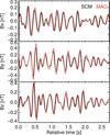 |
Fig. 1 MAG (red) and SCM (black) waveforms in SRF frame, filtered between 3.5 and 8 Hz on September 6 2022 around 15:13:28. |
2 MAG and SCM comparison
2.1 Amplitudes and phases
Figs. 1 and 2 compare the waveforms of MAG and SCM, filtered here between 3.5 Hz and 8 Hz, and between 10 Hz and 20 Hz, respectively. The matching of the waveforms is good but not perfect. We can first see that MAG slightly lags behind the SCM. Second, MAG produces a higher magnetic field than SCM at low frequencies (Fig. 1), with a factor determined to be 14.4% at 1 Hz, and a smaller magnetic field at higher frequencies (Fig. 2). MAG being optimized for low frequencies, its measurements at highest frequencies are more uncertain, especially because of the presence of a low-pass filter to avoid aliasing. At low frequencies (typically below 1 Hz), on the contrary, MAG is accurate and the observed 14% discrepancy can probably be explained by one or a combination of the following factors: uncertainties caused by the very low gain of SCM at these low frequencies, uncertainties in the SCM calibration in temperature, uncertainties caused by the effect of impedance adaptation between SCM and the receivers.
Because of the weak mismatch between MAG and the SCM, we adapt the phases and the amplitudes of the waveforms before performing the merging. These corrections are frequency-dependent, so, we first determine the transfer function between the two instruments, component-wise. For one given day, we divided the SCM waveforms at 256 Hz in small packets of 8 s, took the corresponding MAG burst data (either at 64 or 128 Hz), and performed a cross spectral analysis by estimating for each SRF axis the cross-spectral coherence, the ratio of the Fourier amplitudes between the two instruments, and the cross phase.
In doing so it is important that the magnetic fluctuations exceed the noise floor of each instrument, so we only considered 8 s packets and frequency bins for which the spectral coherence was above 0.95. We repeated this procedure for several days with sufficiently strong magnetic fields fluctuations to increase the statistics and compute average ratios and phase differences for each frequency bin.
Figure 3 shows the results of this procedure, with the ratio between the SCM and MAG amplitudes in the upper panel and the phase difference in the bottom panel. We multiplied SCM amplitudes by 1.144 before the analysis in order to reach a ratio of 1 at 1 Hz. Note that MAG underestimates magnetic field amplitudes at high frequencies, as the result of the low-pass filter of MAG. The origin of the slightly (about 10% near 10 Hz) different amplitude ratio for the three components is unclear. We shall assume when producing the merged magnetic field that SCM is correct at these frequencies and therefore apply these ratios for each component individually. The variation in relative phase shift between components is probably due to a cross-talk between MAG sensor axes, producing apparent delays of a few ms. The linear behaviour of the phase differences between the two instruments below about 10 Hz corresponds to a delay of MAG of about 20 ms, already noted in Figs. 1 and 2, so that the phase difference curves are a combination of this delay and the phase response of MAG at these frequencies.
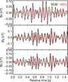 |
Fig. 2 MAG (red) and SCM (black) waveforms in SRF frame, filtered between 10 and 20 Hz on September 6 2022 around 15:13:28. |
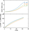 |
Fig. 3 Ratio between SCM and MAG amplitudes (upper panel), and phase difference between SCM and MAG (bottom panel), as a function of frequency and for the three components of the SRF reference frame. The SCM amplitudes have been multiplied by 1.144 in order to have a ratio of 1 at 1 Hz. |
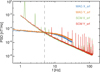 |
Fig. 4 Power spectral density for the Xsrf and Ysrf components of the magnetic field, as measured by MAG and SCM. The Zsrf component is not shown for clarity but is very close to the Ysrf component. |
2.2 MAG and SCM cross-over frequency
Search coil magnetometers are known to have a better detectivity (a lower noise) than flux-gates above typically 1−10 Hz. To better determine the cross-over frequency between the two instruments, we computed their in-flight noise by selecting periods of very low activity in the solar wind. We analysed MAG burst data at 64 Hz and SCM continuous waveforms at 256 Hz from December 132021 to January 22022 and from June 172022 to July 22 2022, during periods when Solar Orbiter was at a distance greater than 0.99 AU from the Sun. Then we down-selected subperiods for which the power spectral density of the magnetic field measured by MAG between 0.5 and 1 Hz was below 2.10−4 nT2/Hz.
Figure 4 shows the power spectral densities for MAG and SCM averaged over these sub-periods. Several interesting features can be noted. First, the sensitivity of the SCM exceeds that of MAG above 5 Hz. At lower frequencies, the SCM noise is higher than expected from ground measurements (not shown) for reasons that are not entirely clear. One of the causes could be the interaction with the Low Frequency Receiver (LFR) of RPW. At higher frequencies, typically above 10 Hz, the apparent decrease in the noise level of MAG is actually caused by low-pass filter that is implemented in MAG to avoid aliasing.
The SCM, which is on the same boom as the two fluxgate instruments but is closer to the satellite platform than the outboard MAG, is sensitive to several spacecraft interferences.
Peaks at 8 Hz, 16 Hz, and harmonics are caused by the Solar Orbiter on-board computer clock and cannot be avoided or corrected as their amplitudes vary in time. They are seen in all three components. Peaks at 1.33 Hz and harmonics appear in Xsrf component only of SCM. Their origin is not clear. Overall, Fig. 4 shows that the merged magnetic field should rely on MAG below approximately 5 Hz and on the SCM above that frequency in order to make the best use of the signal-to-noise ratio of each instrument.
3 MAG and SCM merging procedure
For the merging procedure, we used a similar scheme than the one used for Parker Solar Probe (Bowen et al. 2020). We first estimated the complex Fourier transform of both MAG and SCM waveforms and produced an averaged magnetic field with the following linear combination:
 (1)
(1)
where αscm = 1−αmag and  is the Fourier transform of the merged magnetic field. The noise level of this merged magnetic field is
 (2)
(2)
where  and
and  are the noise levels of MAG and SCM. The frequency transition region from MAG to SCM is therefore controlled by the weights αmag and αscm given to MAG and SCM data. Minimizing Ñ leads to take
 (3)
(3)
The upper panel of Fig. 5 shows αmag (in black) as obtained from Eq. (3) and Fig. 4. At low frequencies, a strict application of this formula leads to weights that are too large for the SCM in a frequency range where its signal is disturbed by interferences at 1.3 Hz and harmonics. It would also lead to non-zero weights for MAG at high frequencies, where its measurements are more often contaminated by its noise. To avoid this, we slightly modified αmag by combining a Butterworth filter of order 3 and a cut-off frequency at 4 Hz, with a decreasing exponential function that is fitted to Eq. (3) between 4 Hz and 10 Hz (the fitting formula is y(f) = 1.34 exp [−(f−0.87)/3.85]). This modified αmag is represented in orange on the top panel of Fig. 5.
The merged magnetic field B is produced from the calibrated magnetic fields measured by MAG and SCM (Level 2 data) in the spacecraft reference frame (SRF) and is subsequently rotated into the RTN frame, when needed. The algorithm first identifies common time intervals of MAG burst data and SCM waveform data at 256 and 4096 Hz. SCM waveforms captured at 24 kHz are not merged since they last only for 83 ms. Continuous time intervals with data from both instruments (separately for 256 and 4096 Hz) are divided into blocks of 4096 SCM points and 32768 SCM points for 256 and 4096 Hz, respectively. The waveforms from MAG are subsequently shifted in time and resampled in Fourier space, using the sampling frequency of SCM. Using the time stamps of SCM as time stamps for the merged data product will ease the joint analysis of magnetic and electric fields as the last one is digitized by the same receiver as SCM. The SCM magnetic field amplitudes are multiplied by 1.144 in order to match the MAG amplitude at 1 Hz. Both MAG and SCM data are then processed in frequency space. The MAG amplitudes are modified according to Fig. 3, meaning that they are corrected only above typically 2 Hz with a factor increasing smoothly to match and follow the SCM amplitudes around 10 Hz and above. The phases of the MAG data are also modified by the phase function, which corrects for the delay observed in Fig. 1. All computations in frequency space are done by first appending the reverse signal (in time) at the end of the original signal to reduce edge effects. Edge effects are further limited by applying the Fourier transform to blocks that overlap by 80% and by keeping only 20% of the data points that are centred in the middle of the blocks.
The lower panel of Fig. 5 shows again the MAG and SCM inflight noise levels for the XSRF component. Also shown is the noise level of the merged magnetic field expected from Eq. (2) and the one computed directly from the merged magnetic field data product over the same common periods used for SCM and MAG. The expected and observed noise level of the merged field are in almost perfect agreement, and the low frequency interferences in the SCM are almost removed in the merged magnetic field. As expected, the noise level of the merged product is that of the MAG below 2 Hz, that of the SCM above 10 Hz, and slightly lower than either in between. Note also that due to the 14% increase in the SCM amplitude to match the MAG at low frequencies, the noise level of the merged magnetic field is 14% higher than that of the SCM alone, although strictly speaking the sensitivity has not been degraded.
Fig. 6 shows the obtained merged magnetic field filtered between 3.5 Hz and 8 Hz for the same case than Fig. 1. As expected, the merged time series are advanced with respect to MAG data and their amplitudes match the ones of MAG. Overall, the behaviour of the observed magnetic field is not altered. At higher frequency (like in Fig. 2), the merged time series are the SCM ones, here again increased by 14%.
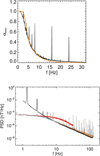 |
Fig. 5 Top panel: αmag used for the merged magnetic field (orange) compared to Eq. (3) (black). Bottom panel: MAG noise (red), SCM noise (black), and computed (blue) and observed (orange) merged noise for the Xsrf component (worst case for SCM). Note that at high frequencies the merged magnetic field has a noise value that 14% above the one from SCM data alone because of the increase in SCM amplitudes to match MAG amplitudes at low frequencies. |
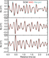 |
Fig. 6 MAG (red), SCM (black), and merged magnetic field (cyan) waveforms in SRF frame, filtered between 3.5 and 8 Hz for the same date than Fig. 1. |
4 The Solar Orbiter merged magnetic field
In this section, we first show some examples of analyses that can be made using this merged magnetic field, and then describe the contents of the merged magnetic field data files.
4.1 Waves and turbulence examples
First, we compare the power spectral density of the merged magnetic field with that obtained from MAG and SCM data. Figure 7 shows two examples computed for September 6 2022. The power spectral density in the top panel is typical of solar wind turbulence with a f−5/3 scaling in the inertial range and a steeper scaling for frequencies beyond the ion scale. Note first that the power spectral density computed with MAG and SCM data alone are barely visible on the figure, indicating that the merged product does not change the original data in the optimal frequency range. We can see the effect of the high pass filter used for calibrating the SCM Level 2 data reduces the contribution from the SCM below typically 3.5 Hz. We can also see that the merged product does not reproduce the lower magnetic power observed by MAG at high frequencies as the result of the anti-aliasing filter, but rather matches the measurements made by the SCM. In the bottom panel, in which we can note in MAG the presence of ion cyclotron waves around 0.2 Hz, we see that the merged magnetic field is reproducing the field measured by SCM at high frequencies and is not contaminated by the noise level of MAG.
The top of Fig. 8 presents the analysis of the merged magnetic field between 0.2 and 128 Hz for several hours on April 4 2024. Solar Orbiter was at 0.29 AU from the Sun. The field was mostly radial (first panel), and the signal above the noise level at all frequency most of the time (second panel). The third panel shows the reduced magnetic helicity (Matthaeus et al. 1982; Alberti et al. 2022),
 (4)
(4)
to highlight the presence of right hand (RH) or left hand (LH) polarized waves. We identify ion cyclotron waves just above 1 Hz, in the frequency range where the transition from MAG to SCM occurs, and whistler waves above 10 Hz. The last panel shows two power spectral densities, one in black computed for periods without ion cyclotron waves (ICWs), and one in red for periods with ion cyclotron waves. Periods with ICWs (red spectrum) were identified as periods for which the averaged reduced magnetic helicity between 1 and 3 Hz was less than −0.15. Periods without ICWs (black spectrum) were identified as periods for which the absolute value of this averaged reduced magnetic helicity was less than 0.05. For clarity, the power spectral density in red has been increased by 30% in order to match the level of the black one at 0.01 Hz. The simultaneous presence of ion cyclotron waves and a drop in the power spectral density at sub-ion scales support the recently observed drop in cascading energy observed by Parker Solar Probe (Bowen et al. 2024).
Figure 9 shows a similar analysis, but for a merged magnetic field with a sampling frequency of 4096 Hz. These data were obtained by the Solar Orbiter at 0.71 AU from the Sun. The presence of RH waves (BR is negative), which we identify as whistler waves since they have been frequently observed in the solar wind and by Solar Orbiter (Lacombe et al. 2014; Jagarlamudi et al. 2020; Kretzschmar et al. 2021; Colomban et al. 2024), is clearly visible before 13:27, while turbulence increases after that time. The lower panel shows the power spectral density averaged between 1:23:30 and 1:27:00 in orange and a power spectral density averaged between 1:27:40 and 1:29:16 in black. Both spectra show an inertial range with a Kolmogorov scaling f−5/3, as well as a flattening of the power spectral densities before a steeper scaling in the kinetic regime. However, there is also a break in the cascade around 200 Hz, at frequencies close to the one at which whistler activity is observed at earlier times. Further analysis is required to interpret these results, but this once again demonstrates the potential of this merged magnetic field data product for the analysis of waves and turbulence from the fluid scale down to the ion and electron scales.
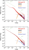 |
Fig. 7 Top panel: power spectral density of the magnetic field computed for September 6 2022 between 2:30pm and 3:30pm, using L2 MAG burst data (black), L2 SCM data (orange), and the merged magnetic field (red). The purple curve is the noise level of the merged product. The f−5/3 and f−8/3 (8/3=2.66) scaling are indicated for visual comparison. Bottom panel: power spectral density for the same day, but between 21:30 and 22:30. |
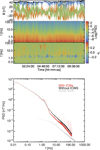 |
Fig. 8 Top: waveforms (radial component in blue, tangential in orange, normal in green, modulus in black), power spectral density, and reduced helicity σr of the merged magnetic field at 256 Hz on April 4 2024. Bottom: power spectral densities for σr ≃ 0 (black) and negative σr (red). |
4.2 Content of the Solar Orbiter merged magnetic field data product
The merged magnetic field data product is distributed as Common Data Format (CDF) files on the Solar Orbiter Archive1. The sampling frequency is either 256 Hz or 4096 Hz and the reference frame is either SRF or RTN. Four different CDF files cover these four cases for a given day.
For a given frame and sampling frequency, the merged magnetic field can be produced from MAG burst data at 64 Hz or 128 Hz (the two are possible within one day and therefore within one file) on one side and SCM snapshot or continuous waveform on the other side. As described earlier, the merging is done over periods of continuous SCM data intervals, with overlapping blocks. In cases where SCM snapshot waveforms were used in the merging, there is no overlapping in the merging process and the continuous intervals and the blocks have the same length of 2048 SCM points. When continuous waveforms from the SCM are used, the continuous intervals can have durations from a few minutes to several hours. We do not expect, and have not found, differences in the merged magnetic field depending on the type of MAG and SCM data used. A comparison of the original MAG data with the merged magnetic field near the edges of the blocks has not shown that the DC field has been altered. However, despite the care taken with the merging procedure, the merged DC magnetic field may be less accurate near the edges of continuous time intervals.
Table 1 lists the variables contained in the merged magnetic field data product. Beyond time and magnetic fields, the CDF files includes the important variable MERGED_BITMASK whose the value indicates what kind of inputs data were used. The variable MERGED_LABEL is the textual corresponding information. Whenever the value of MERGED_BITMASK is changing, or if there are gaps in SCM data and therefore in the merged magnetic field data, a new block is considered. The variable QUALITY_BITMASK_MAG and QUALITY_BITMASK_SCM are reproduced from the original MAG and SCM data files and can be used to find the relevant caveats related to each instrument.
The temporal coverage of the dataset is shown on Fig. 10; on average, the merged magnetic field at 256 Hz exists for 8 h/day. The availability of the merged magnetic field depends on both the availability of MAG BURST data and SCM snapshot or continuous waveforms at 256 or 4096 Hz (survey or burst). Therefore, the unavailability of the merged magnetic field does not mean that one or the other kind of data does not exist but that the two were not available at the same time.
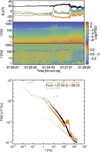 |
Fig. 9 Top: time series, Power spectral density, and reduced helicity σr of the merged magnetic field at 4096 Hz on September 4 2022. Bottom: two power spectral densities with and without waves. Noise level is indicated in grey. Scaling of f−5/3 and f−8/3 are indicated for visual comparison. |
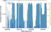 |
Fig. 10 Daily temporal coverage of the merged magnetic field at 256 Hz (blue) and 4096 Hz (purple) together with the heliocentric distance of Solar Orbiter (orange). |
Content of the merged magnetic field Common Data Format (CDF) files.
5 Conclusions
We have carried out a detailed analysis of the Solar Orbiter mission’s fluxgate and search coil magnetometers in their overlapping frequency range. This has allowed us to produce a merged magnetic field data product that preserves the best of both instruments and covers frequencies from DC to 2048 Hz (Nyquist frequency). We have shown that the merged data is suitable for analysing waves and turbulence over a wide frequency range. The Solar Orbiter merged magnetic field is openly distributed as CDF files through the usual databases.
Acknowledgements
Solar Orbiter is a space mission of international collaboration between ESA and NASA, operated by ESA. We acknowledge the support from the Centre National d’Etudes Spatiales (CNES, French space agency) for this study and the development, calibration, and operation of the search soil magnetometer of RPW. Solar Orbiter magnetometer (MAG) operations are funded by the UK Space Agency (grant ST/T001062/1). T.H. is supported by STFC grant ST/S000364/1.
References
- Alberti, T., Narita, Y., Hadid, L. Z., et al. 2022, A&A, 664, L8 [NASA ADS] [CrossRef] [EDP Sciences] [Google Scholar]
- Alexandrova, O., Mangeney, A., Maksimovic, M., et al. 2004, J. Geophys. Res., 109, A05207 [Google Scholar]
- Alexandrova, O., Saur, J., Lacombe, C., et al. 2009, Phys. Rev. Lett., 103, 165003 [NASA ADS] [CrossRef] [Google Scholar]
- Argall, M. R., Fischer, D., Le Contel, O., et al. 2018, ArXiv eprints [arXiv:1809.07388] [Google Scholar]
- Bowen, T. A., Bale, S. D., Bonnell, J. W., et al. 2020, J. Geophys. Res., 125, e27813 [Google Scholar]
- Bowen, T. A., Bale, S. D., Chandran, B. D. G., et al. 2024, Nat. Astron., 8, 482 [Google Scholar]
- Chen, C. H. K., Horbury, T. S., Schekochihin, A. A., et al. 2010, Phys. Rev. Lett., 104, 255002 [NASA ADS] [CrossRef] [Google Scholar]
- Chen, C. H. K., Bale, S. D., Bonnell, J. W., et al. 2020, ApJS, 246, 53 [Google Scholar]
- Chust, T., Kretzschmar, M., & Graham, D., 2021, A&A, 656, A17 [NASA ADS] [CrossRef] [EDP Sciences] [Google Scholar]
- Colomban, L., Kretzschmar, M., Krasnoselkikh, V., et al. 2024, A&A, 684, A143 [NASA ADS] [CrossRef] [EDP Sciences] [Google Scholar]
- Durrant-Whyte, H., & Henderson, T. C., 2008, in Springer Handbook of Robotics, eds. B. Siciliano, & O. Khatib (Berlin: Springer-Verlag), 585 [Google Scholar]
- Fischer, D., Magnes, W., Hagen, C., et al. 2016, GI, 5, 521 [Google Scholar]
- Gary, S. P., & Feldman, W. C., 1977, J. Geophys. Res., 82, 1087 [NASA ADS] [CrossRef] [Google Scholar]
- Horbury, T. S., Forman, M., & Oughton, S., 2008, Phys. Rev. Lett., 101, 175005 [Google Scholar]
- Horbury, T. S., O’Brien, H., Carrasco Blazquez, I., et al. 2020, A&A, 642, A9 [NASA ADS] [CrossRef] [EDP Sciences] [Google Scholar]
- Jagarlamudi, V. K., Alexandrova, O., Berčič, L., et al. 2020, ApJ, 897, 118 [Google Scholar]
- Jannet, G., Dudok de Wit, T., Krasnoselskikh, V., et al. 2021, J. Geophys. Res., 126, e2020JA028543 [Google Scholar]
- Kretzschmar, M., Chust, T., Krasnoselskikh, V., et al. 2021, A&A, 656, A24 [NASA ADS] [CrossRef] [EDP Sciences] [Google Scholar]
- Lacombe, C., Alexandrova, O., Matteini, L., et al. 2014, ApJ, 796, 5 [Google Scholar]
- Lacombe, C., Alexandrova, O., & Matteini, L., 2017, ApJ, 848, 45 [Google Scholar]
- Maksimovic, M., Bale, S. D., Chust, T., et al. 2020, A&A, 642, A12 [EDP Sciences] [Google Scholar]
- Malaspina, D. M., Ergun, R. E., Cairns, I. H., et al. 2024, ApJ, 969, 60 [Google Scholar]
- Matthaeus, W. H., Goldstein, M. L., & Smith, C., 1982, Phys. Rev. Lett., 48, 1256 [Google Scholar]
- Müller, D., Cyr, O. C. St., Zouganelis, I., et al. 2020, A&A, 642, A1 [NASA ADS] [CrossRef] [EDP Sciences] [Google Scholar]
- Sahraoui, F., Goldstein, M. L., Robert, P., & Khotyaintsev, Y. V., 2009, Phys. Rev. Lett., 102, 231102 [NASA ADS] [CrossRef] [Google Scholar]
- Scime, E. E., Bame, S. J., Feldman, W. C., et al. 1994, J. Geophys. Res., 99, 23401 [Google Scholar]
- Shankarappa, N., Klein, K. G., Martinović, M. M., & Bowen, T. A., 2024, ApJ, 973, 20 [Google Scholar]
https://doi.org/10.57780/esa-f2565a8 and will soon be available. In the meantime, data used in this paper are available here, and users can obtain more data on demand by writing to the authors
All Tables
All Figures
|
Fig. 1 MAG (red) and SCM (black) waveforms in SRF frame, filtered between 3.5 and 8 Hz on September 6 2022 around 15:13:28. |
| In the text | |
|
Fig. 2 MAG (red) and SCM (black) waveforms in SRF frame, filtered between 10 and 20 Hz on September 6 2022 around 15:13:28. |
| In the text | |
|
Fig. 3 Ratio between SCM and MAG amplitudes (upper panel), and phase difference between SCM and MAG (bottom panel), as a function of frequency and for the three components of the SRF reference frame. The SCM amplitudes have been multiplied by 1.144 in order to have a ratio of 1 at 1 Hz. |
| In the text | |
|
Fig. 4 Power spectral density for the Xsrf and Ysrf components of the magnetic field, as measured by MAG and SCM. The Zsrf component is not shown for clarity but is very close to the Ysrf component. |
| In the text | |
|
Fig. 5 Top panel: αmag used for the merged magnetic field (orange) compared to Eq. (3) (black). Bottom panel: MAG noise (red), SCM noise (black), and computed (blue) and observed (orange) merged noise for the Xsrf component (worst case for SCM). Note that at high frequencies the merged magnetic field has a noise value that 14% above the one from SCM data alone because of the increase in SCM amplitudes to match MAG amplitudes at low frequencies. |
| In the text | |
|
Fig. 6 MAG (red), SCM (black), and merged magnetic field (cyan) waveforms in SRF frame, filtered between 3.5 and 8 Hz for the same date than Fig. 1. |
| In the text | |
|
Fig. 7 Top panel: power spectral density of the magnetic field computed for September 6 2022 between 2:30pm and 3:30pm, using L2 MAG burst data (black), L2 SCM data (orange), and the merged magnetic field (red). The purple curve is the noise level of the merged product. The f−5/3 and f−8/3 (8/3=2.66) scaling are indicated for visual comparison. Bottom panel: power spectral density for the same day, but between 21:30 and 22:30. |
| In the text | |
|
Fig. 8 Top: waveforms (radial component in blue, tangential in orange, normal in green, modulus in black), power spectral density, and reduced helicity σr of the merged magnetic field at 256 Hz on April 4 2024. Bottom: power spectral densities for σr ≃ 0 (black) and negative σr (red). |
| In the text | |
|
Fig. 9 Top: time series, Power spectral density, and reduced helicity σr of the merged magnetic field at 4096 Hz on September 4 2022. Bottom: two power spectral densities with and without waves. Noise level is indicated in grey. Scaling of f−5/3 and f−8/3 are indicated for visual comparison. |
| In the text | |
|
Fig. 10 Daily temporal coverage of the merged magnetic field at 256 Hz (blue) and 4096 Hz (purple) together with the heliocentric distance of Solar Orbiter (orange). |
| In the text | |
Current usage metrics show cumulative count of Article Views (full-text article views including HTML views, PDF and ePub downloads, according to the available data) and Abstracts Views on Vision4Press platform.
Data correspond to usage on the plateform after 2015. The current usage metrics is available 48-96 hours after online publication and is updated daily on week days.
Initial download of the metrics may take a while.