| Issue |
A&A
Volume 642, October 2020
The Solar Orbiter mission
|
|
|---|---|---|
| Article Number | A12 | |
| Number of page(s) | 23 | |
| Section | Astronomical instrumentation | |
| DOI | https://doi.org/10.1051/0004-6361/201936214 | |
| Published online | 30 September 2020 | |
The Solar Orbiter Radio and Plasma Waves (RPW) instrument
1
LESIA, Observatoire de Paris, Université PSL, CNRS, Sorbonne Université, Univ. Paris Diderot, Sorbonne Paris Cité, 5 Place Jules Janssen, 92195 Meudon, France
e-mail: milan.maksimovic@obspm.fr
2
Space Sciences Laboratory, University of California, Berkeley, CA, USA
3
Physics Department, University of California, Berkeley, CA, USA
4
Stellar Scientific (now HELIOSPACE), 932 Parker St suite 2, Berkeley, CA 94710, USA
5
LPP, CNRS, Ecole Polytechnique, Sorbonne Université, Observatoire de Paris, Université Paris-Saclay, PSL Research University, Palaiseau, Paris, France
6
LPC2E, CNRS, 3A Avenue de la Recherche Scientifique, Orléans, France
7
Université d’Orléans, Orléans, France
8
Technische Universität Dresden, Würzburger Str. 35, 01187 Dresden, Germany
9
Space Research Institute, Austrian Academy of Sciences, Graz, Austria
10
Institute of Atmospheric Physics, Czech Academy of Sciences, Prague 14131, Czech Republic
11
Astronomical Institute, Czech Academy of Sciences, 14100 Prague, Czech Republic
12
Swedish Institute of Space Physics (IRF), Uppsala, Sweden
13
Nexeya Conseil et Formation, 5 Rue Boudeville ZI de Thibaud, 31100 Toulouse, France
14
CNES, 18 Avenue Edouard Belin, 31400 Toulouse, France
15
Logiqual, Avenue Didier Daurat, 31700 Blagnac, France
16
Altran Sud Ouest 4, Avenue Didier Daurat, 31700 Blagnac, France
17
Université de Rennes, 1 – 263 Avenue du Général Leclerc, 35042 Rennes, France
18
Faculty of Mathematics and Physics, Charles University, Prague, Czech Republic
19
Universities Space Research Association, Columbia, MD, USA
20
ASA Goddard Space Flight Center, Greenbelt, MD, USA
21
Department of Space and Plasma Physics, School of Electrical Engineering and Computer Science, Royal Institute of Technology, Stockholm, Sweden
22
Department of Physics and Astronomy, University of Calgary, Calgary, Alberta, Canada
23
School of Physics and Astronomy, University of Minnesota, Minneapolis, MN, USA
24
Department of Physics, Imperial College, SW7 2AZ London, UK
25
School of Astronomy and Astrophysics, Glasgow University, Glasgow, UK
26
University of Applied Sciences and Arts Northwestern Switzerland, 5210 Windisch, Switzerland
27
IRAP, CNRS, Universit de Toulouse, UPS, Toulouse, France
28
Lunar and Planetary Laboratory, University of Arizona, Tucson, AZ 85719, USA
29
Department of Astronomy, Faculty of Mathematics, University of Belgrade, Studentski trg 16, 11000 Belgrade, Serbia
30
Mullard Space Science Laboratory, University College London, Holmbury St. Mary, Dorking RH5 6NT, UK
31
Space Research Group, Universidad de Alcala, Alcala de Henares, Spain
32
Institute of Experimental and Applied Physics, Christian-Albrechts-University, Kiel, Germany
33
ESA, ESAC, Madrid, Spain
34
Radboud Radio Lab, Department of Astrophysics/IMAPP – Radboud University, PO Box 9010, 6500 GL Nijmegen, The Netherlands
35
Commission for Astronomy, Austrian Academy of Sciences, Graz, Austria
Received:
29
June
2019
Accepted:
30
January
2020
The Radio and Plasma Waves (RPW) instrument on the ESA Solar Orbiter mission is described in this paper. This instrument is designed to measure in-situ magnetic and electric fields and waves from the continuous to a few hundreds of kHz. RPW will also observe solar radio emissions up to 16 MHz. The RPW instrument is of primary importance to the Solar Orbiter mission and science requirements since it is essential to answer three of the four mission overarching science objectives. In addition RPW will exchange on-board data with the other in-situ instruments in order to process algorithms for interplanetary shocks and type III langmuir waves detections.
Key words: solar wind / instrumentation: miscellaneous
© M. Maksimovic et al. 2020
 Open Access article, published by EDP Sciences, under the terms of the Creative Commons Attribution License (https://creativecommons.org/licenses/by/4.0), which permits unrestricted use, distribution, and reproduction in any medium, provided the original work is properly cited.
1. Introduction
The Radio and Plasma Waves (RPW) instrument on the ESA Solar Orbiter mission (Müller et al. 2020) is designed to measure magnetic and electric fields, plasma wave spectra and polarization properties, the spacecraft (S/C) floating potential and solar radio emissions in the interplanetary medium.
More specifically, RPW will measure the three-component magnetic field fluctuations from about 10 Hz to a few hundred of kHz to fully characterize magnetized plasma waves in this range. Three electric antennas will be combined to retrieve the local plasma potential and to produce two components of the direct current (DC) ambient electric field in the solar wind. RPW will also observe solar radio emissions up to 16 MHz and the associated Langmuir waves around the local plasma frequency occasionally. Finally, the instrument radio receiver will detect the local quasi-thermal noise providing good measurements of the in-situ absolute electron density and temperature, when the ambient plasma Debye length will be adequate. The RPW instrument is of primary importance to the Solar Orbiter mission and science requirements (Müller et al. 2020) since it is essential to answer three of the four mission overarching science objectives. Moreover, the scientific goals of the RPW instrument fall in the general Solar Orbiter science activity plan (Zouganelis et al. 2020).
In the following section, we briefly describe the specific RPW science objectives and requirements. In Sect. 3 we describe the instrument design and subsystems exhaustively. In Sect. 4 we focus on the RPW flight software, and finally in Sect. 5 we briefly describe the operations concept and the RPW data products in Sect. 6.
2. The RPW science objectives and measurements requirements
The science objectives described in this section rely on characteristic plasma frequencies and scales that are expected to vary with heliocentric distance over the course of the Solar Orbiter mission. Figure 1 displays these variations. RPW will operate permanently during the course of the scientific mission and down to 0.28 astronomical unit (AU), which will be the closest perihelion the Solar Orbiter will reach.
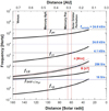 |
Fig. 1. Variations with Heliocentric distance of the characteristic plasma frequencies. Are also indicated the instrument various sampling frequencies (see Sect. 3.4 for more details). |
2.1. Low frequency measurements and turbulence
Despite more than a half-century of study and space exploration, the basic physical processes responsible for heating and acceleration of the solar wind are still not understood well. It is generally believed that complex mechanisms that couple particles and electromagnetic fluctuations, in the form of waves or coherent structures (Sperveslage et al. 2000; Greco et al. 2009; Tsurutani et al. 2011; Lion et al. 2016) are at the origin of these processes. The solar wind is a turbulent flow (Bruno & Carbone 2013) with fluctuations in the electromagnetic field and particle bulk velocities (and other parameters) over a wide range of scales extending to ion and electron characteristic scales where energy of these turbulent fluctuations are likely dissipated and transferred to particles (Alexandrova et al. 2013). Furthermore, particle distribution functions in the weakly collisional solar wind plasma exhibit strong departures from thermal equilibrium (owing to the interaction with electromagnetic fluctuations as well as to the solar wind expansion into space). These departures may lead to instabilities that modify the particle distribution functions, bound the particle parameter space (Hellinger et al. 2006; Matteini et al. 2007; Štverák et al. 2008; Maruca et al. 2012), and redistribute energy between electromagnetic fluctuations and, generally different, particle species (Matteini et al. 2012).
RPW will characterize the radial evolution of both the magnetic and the electric components of the solar wind turbulence up to the electron scales. The instrument will also identify the different instabilities that affect the solar wind particle distribution functions and in particular their energetics using its low frequency electric and magnetic fields measurements and explore their propagation properties (wave vectors determinations, polarizations ...) and their radial and latitudinal evolutions in the ranges covered by the mission and which correspond to 0.28 to 1 AU and −35° to +35° heliolatitude.
2.2. Quasi-thermal noise spectroscopy
The accurate in-situ measurement of the solar wind electron properties is a key element in understanding the physics of the solar wind. For this purpose, the quasi-thermal noise (QTN) spectroscopy technique is very robust since it is based on the use of a passive electric antenna for measuring the electrostatic field spectrum produced by the electron and ion thermal motions in a stable plasma (Meyer-Vernet et al. 2017). One should also notice that the density measurement is independent of any calibration or gain determination, since it relies directly on a frequency measurement which its relies on an internal instrument frequency clock, which is well know.
The QTN spectroscopy requires an antenna length L larger than the local Debye length LD, in order to measure adequately the electron temperature. In addition, the antenna must have a radius much smaller than LD in order to minimize the shot noise (Meyer-Vernet et al. 2017). With a 6.5 m antenna length, which is the case for RPW, these conditions should be met for all the denser solar winds, having a density of about 10 cm−3 or higher at 1 AU (Maksimovic et al. 2001). In that case, the electron density determination from the thermal noise peak will be done with at least a 3% of accuracy (Maksimovic et al. 1995, 1998).
2.3. Solar radio emissions
One of the major challenges in solar radio astronomy is that all solar radio burst sources are embedded into magnetized turbulent plasma, so the observed emissions are affected by radio wave propagation. Specifically, radio waves are strongly scattered in the solar corona and an apparent source seems to be larger than the actual source. In addition, the scattering and refraction shifts the positions of the sources. Recently, the observations with the LOw Frequency ARray (LOFAR) with unprecedented temporal and frequency resolutions demonstrate that the scattering on density fluctuations is the key process in the interpretation of solar radio images (Kontar et al. 2017). While the origin of the density fluctuations observed in solar radio bursts (Chen et al. 2018) is strongly debated (Krupar et al. 2018; Sharykin et al. 2018), the spectrum of density fluctuations is essential to simulate radio wave transport (Krupar et al. 2018). Since the effect of radio wave scattering depends on the poorly-known spectrum of density turbulence in the solar atmosphere (Thejappa & MacDowall 2008), RPW will substantially improve our understanding of the radio wave propagation by providing much needed in-situ information on the density fluctuations. Furthermore, RPW observations jointly with ground based radio observatories such as the Nancay Decameter Array and Radio Heliograph, LOFAR or the future Square Kilometer Array (SKA) will also address the nature of the compressive density fluctuations in the inner heliosphere, which is also a central question for the corona heating problem.
RPW will also measure intense in situ Langmuir-like waves which are frequently observed in the solar wind in association with suprathermal electron beams produced by either solar flares (Lin et al. 1981) or accelerated by interplanetary shocks (Bale et al. 1999). These waves are believed to undergo linear mode conversion and/or nonlinear wave-wave interactions that produce electromagnetic emissions at the local electron plasma frequency fpe and its second harmonic 2fpe (Melrose 1982). RPW offers unique opportunities to study this latter problem by making new measurements of both the electric and magnetic fluctuations at the local plasma frequency and by retrieving the waves phase speed Vϕ from the ratio of fluctuations δE/δB. By comparing Vϕ with the local o-, x-, and z-mode wave speeds, RPW will reveal primary evidence of mode-coupling and conversion of Langmuir waves into electromagnetic Type II or Type III radiations.
In addition to the science topics above, RPW will address several other including interplanetary shocks, magnetic reconnection, current sheets or interplanetary and interstellar dust detection. Those do not specifically drive the RPW measurement requirements described below but will be made possible to sudy given how the instrument is designed.
2.4. RPW measurement requirements
In order to fulfill its science objectives RPW has to provide both waveform and spectral data with sensitivities and dynamical ranges displayed in Figs. 2–4.
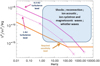 |
Fig. 2. Various natural phenomena that will be observed by the RPW instrument in the DC–LF frequency range and associated sensitivity and dynamical range requirements. The spectral breaks are assumed to occur at proton and electron gyro-frequencies (see text for more details). |
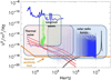 |
Fig. 3. Various natural phenomena that will be observed by the RPW instrument in the radio domain and associated sensitivity and dynamical range requirements (see text for more details). As far as the QTN is concerned one can note that because we will be in a regime where the antenna length is comparable to the Debye length, the plasma peaks are not prominent and do not appear visible on this figure. |
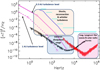 |
Fig. 4. Magnetic field fluctuations of various natural phenomena that will be observed by the RPW instrument and associated sensitivity and dynamical range requirements. The spectral breaks are assumed to occur at proton and electron gyro-frequencies (see text for more details). |
Figure 2 displays various natural electric waves that will be observed by RPW in the quasi DC/LF (Direct Current Low Frequency) range up to 10 kHz and described in the previous section. This range covers the electron gyro-frequency and most of the Doppler-shifted frequencies of the low frequency plasma waves. Assuming Alfvénic like waves, the electric counterpart of the solar wind magnetic turbulence levels is displayed for typical 1 AU conditions by the dashed pink curve with stars and for expected turbulence levels at 0.3 AU by the pink curve with diamonds. The blue box summarizes the range of intensities of the various kind of waves that play a role in the solar wind physics and that will be observed by RPW.
The orange curve represents the required RPW sensitivity level for the electric field measurements. This sensitivity level would allow to measure the solar wind turbulence spectra down to the electron dissipation range (the last section of pink lines) and to measure all the expected plasma waves in the given frequency range.
Figure 3 displays the various natural electric waves that will be observed by RPW in the radio frequency range from about 10 kHz up to about 16 MHz and described in the previous section. The set of red curves between 4 kHz and 1 MHz are the simulated levels for the Quasi Thermal Noise measurement which will provide the ambient electron density and temperature. These curves have been obtained for the following densities and temperatures: Ne = 3 cm−3 and Te = 105 K which is typical of the fast wind at 1 AU; Ne = 100 cm−3 and Te = 3 × 10⁵ K for the slow wind at 0.3 AU; Ne = 30 cm−3 and Te = 2 × 10⁵ K which is intermediate between the two latter and, finally, Ne = 200 cm−3 and Te = 105 K which is typical for a dense and cold magnetic cloud at 0.3 AU.
The black curve on Fig. 3 represents the galactic noise level as observed with a 6.5 m long antenna monopole, corresponding to the RPW configurations.
Another interesting dataset for setting the RPW requirements in this frequency range is the one provided by the WIND/WAVES instrument (Bougeret et al. 1995). The full and dashed blue lines in the 4 to 256 kHz frequency range represent the minimum and maximum power spectral densities recorded by WAVES over 14 years of operations from 1995 to 2009. Typical values for Type III associated Langmuir waves intensities are represented by the green points and typical intensities for the Type III radio emissions by the blue dots.
Finally, Fig. 4 displays the magnetic sensitivity of the RPW Search Coil Magnetometer (SCM), described in Sect. 3.2, together with the magnetic field fluctuations of various natural phenomena which will be observed by RPW. The SCM sensitivity measurements have been performed in laboratory with a 1 Hz bandwidth for the low-frequency mono-band coil (black curve) and the high-frequency bi-band coil (red curve).
The solar wind magnetic turbulence levels are displayed in Fig. 4 for typical 1 AU observations (dashed pink curve with stars) and for expected turbulence levels at 0.3 AU (pink curve with diamonds). These turbulence levels come from the studies by Bruno et al. (2005) and Alexandrova et al. (2009, 2020). It can be seen that with the SCM mono-band coil, it will be possible to measure the expected turbulence levels below 100 Hz at 1 AU and up to 2 kHz at 0.3 AU.
The blue line represents the maxima of the magnetic level values observed by the search coil magnetometer of the HELIOS S/C (Dehmel et al. 1975) between 0.3 and 1 AU over the course of its mission (Dudok de Wit, priv. comm.). These values correspond to the strong magnetic fluctuations within interplanetary shocks, reconnection events, whistler turbulence as observed by HELIOS.
Finally, the pink box, covering frequencies from 104 Hz to 106 Hz, represents the expected amplitude range of the magnetic component of radio waves and Langmuir-like waves associated with type II and type III radio emissions.
2.5. Electromagnetic Cleanliness requirements
The electric and magnetic sensitivities required for RPW and displayed in Figs. 2–4 necessitate the global S/C (platform and other instruments) potential disturbances to be minimized. To accommodate this, a S/C level Electromagnetic Cleanliness (EMC) program has been established and requirements at system level have been set. At instrument level auto-compatibility tests have been carried out between the RPW Search Coil (see section below) and the Magnetometer (MAG) instrument (Horbury et al. 2020), which are both sitting on the instrument boom. These ground tests have demonstrated that the two instruments are compatible. Also the S/C reaction wheels have been shielded on purpose to avoid pollution by magnetic spurious drifting frequencies. EMC characterizations of all payload and S/C subsystems have been conducted after the building phases and has provided a global picture which will need to be confirmed in space. Finally operational EMC quiet periods have been introduced in the mission Science Activity Plan (Zouganelis et al. 2020).
3. Instrument design
The RPW instrument is composed of three main subsystems whose accommodation on the Solar Orbiter S/C (García-Marirrodriga et al. 2020) is illustrated on Fig. 5.
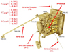 |
Fig. 5. Payload accommodation on Solar Orbiter S/C. The RPW sub-units are indicated in red. The electric Antenna system (ANT) consists of a set of three identical antennas deployed from +Z axis (Antenna PZ) and from the opposite corners of the S/C +Y and -Y walls (Antennas PY and MY). The SCM consists of a set of three magnetic antennas mounted orthogonally. Their orientations, in the S/C reference frame, are given by the three vectors in the upper left part of the figure. Finally the Main Electronic Box (MEB) is located inside the S/C body. |
The electric Antenna system (ANT) consists of a set of three identical antennas deployed from +Z axis (Antenna PZ) and from the opposite corners of the S/C +Y and -Y walls (Antennas PY and MY). The Search-Coil Magnetometer (SCM) is located on the Solar Orbiter instrument boom 2 m away from the S/C, for electromagnetic compatibility (EMC) reasons. Finally a Main Electronics Box (MEB), which collects all the signals coming from the ANT and SCM preamplifiers, is located inside the S/C body.
In the following subsections these three subsystems are described in details.
3.1. The electric antenna (ANT) design
The three RPW electric antennas consist each of a 1 m rigid deployable boom and a 6.5 m stacer deployable monopole which is actually the electric sensor itself. Figure 6 shows the antenna design in both stowed and deployed configurations.
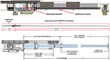 |
Fig. 6. From top to bottom: antenna overview in stowed configuration. Antenna dimensions one deployed. Main dimensions of the deployed stacers (in meter) with the conductive part of the sensor indicated in blue. |
The boom assembly consists of a hinge assembly partly made of titanium, a carbon fiber tube, and a stacer adapter and frame. This latter serves to support the stacer assembly as well as the deployment assist device and thermal shields.
The stacers are spring elements consisting of a helically wound, 127 mm wide by 0.1 mm thick flat metal strip formed into a helix. The helix is collapsed into itself during stowing, such that the stowed stacer fits into a canister equal in length to the strip width and 51 mm in diameter when extended. The stacer overlapping coil grips the previous, forming a tapered thin-walled tube. The stacers are formed from Elgiloy, a nickel cobalt super alloy.
The boom and stacer deployments are commanded separately. Once the boom has completed its ninety degree rotation, a latch engages to hold the boom erect under maneuvering loads. The stacer monopole is then deployed by means of a commanded Frangibolt. The stacer deploys under its own power until it reaches the end of travel, with its speed and final length controlled by means of a cable and a flyweight brake. A set of heat shields protect the boom, mechanisms, and preamp from the solar flux once deployed
Figure 7 shows the three antenna units dimensions and configurations once deployed, together with their naming conventions. Note that the three angles between the three couples of monopoles are not perfectly equal and that a bending of the antennas will occur in flight due to thermoelastic distortion. This bending will be different for the three antennas, depending on their own temperatures. Preliminary modeling of this bending shows that at closest approach the tip of the antennas can be shifted up to 1.5 m from its mechanical position at rest.
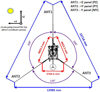 |
Fig. 7. Three antenna units dimensions and configurations once deployed. |
3.1.1. The electric antenna preamplifiers design
Each preamplifier and its thermal screen are fixed on the stacer frame as close as possible to the antenna part. Between the arm and the antenna, a ceramic device insures electrical and thermal insulation. The preamplifier box is protected from the Sun even in OFF pointing of the S/C by the antenna heatshield made up of Niobium.
Figure 8 displays the preamplifiers electrical design. In order to make a high quality measurement in the wide frequency range from DC up to 16 MHz, the signal from antennas is split in Low Frequency (LF) and High Frequency (HF) parts that are amplified separately and which later feed the LF and HF analysis parts of RPW instrument.
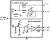 |
Fig. 8. Antenna preamplifiers electrical design. See text for more details. |
In the LF part of the preamplifier, the relay is used to perform the bias current calibration by connecting the input to a calibration resistor Rcal instead of the antenna (see also Fig. 20). In addition, the in-flight calibration verification of the signal path from preamplifier to the Low Frequency Receiver (LFR) and the Time Domain Sampler (TDS) will be required to adjust the bias settings of antennas. It is carried out by measuring the bias current voltage drop across the resistor on the preamplifier input, selected by the same relay.
For the high frequency signals, a wide input dynamic range and a good linearity are needed to make accurate measurements, such as the QTN measurements or plasma wave polarization and dynamics.
3.1.2. Electric Antennas calibrations and characteristics
The RPW antennas have been designed in order to fulfill the science objectives of the instrument both in the DC-LF and radio domains. This design has been assessed on ground, prior to launch, by both simulations and measurements. This assessment is described in details in Maksimovic (2019) where the pre-launch performances of the whole instrument are described. For the low frequency measurements and especially for the DC electric field ones, simulations effort are ongoing at the time of submitting this article. For the radio part Fig. 9 summarizes the characteristics obtained after ground testing and characterizations. Figure 10 details the various contributions to the antenna stray capacitance.
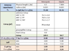 |
Fig. 9. Antenna radio-electrical properties. |
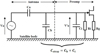 |
Fig. 10. Various contributions to the antenna stray capacitance. We note that Va′ is the measured voltage while Va is the natural voltage in the plasma. |
Note, finally, that the actual antennas properties and final calibrations will be performed in the Solar Wind with a fully operating S/C and RPW instrument.
3.2. The Search Coil Magnetometer (SCM)
The Search Coil Magnetometer (SCM) will measure the three components of the solar wind magnetic fields fluctuations, from 10 Hz to 10 kHz as well as from 10 kHz to 500 kHz in one direction only. The bandwidth and dynamic range of the instrument will provide crucial data for the investigations of interplanetary shocks, reconnections, turbulence, wave-particle interactions and plasma wave in general. The SCM instrument consists of a triaxial search-coil that has a solid heritage on several other missions such as the TARANIS (Lefeuvre et al. 2008) or Parker Solar Probe (Fox et al. 2016). The instrument is composed of 3 antennas made of a magnetic core with a winding whose voltage is proportional to the time-derivative of the magnetic field. Two antennas of SCM cover the low frequency (hereafter LF) range from 10 Hz to 10 kHz. The third one is a dual-band antenna that covers the medium frequency (hereafter MF) range from 10 kHz to 500 kHz. The three antennas, each of which is 104 mm long, are mounted orthogonally on a non-magnetic support, as shown on Fig. 11. The orientations of the three SCM antennas are provided on Fig. 5 in the S/C reference frame. The dual-band antenna is +XSCM.
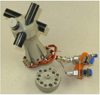 |
Fig. 11. Flight model of the search-coil magnetometer. |
As a consequence of the SCM accommodation on the satellite’s instrument boom, the sensor will remain in the shadow of the thermal shield at about −55°C. Note that the sensor may encounter much colder conditions if no particular precaution are taken (such as an external heating by the platform which is currently planned). Several optimizations were thus done in order to achieve technical (mass, volume, power consumption) and scientific (gain, noise level) performances despite of the very low temperature environment.
The material of the magnetic core in the antennas has been selected and tested for its ability to maintain the characteristics at low temperatures. Heaters have been implemented around the preamplifier to maintain it in its acceptable temperature range. In addition, to mitigate thermal losses of the instrument, the instrument is wrapped in a double 15 multi-layer insulation (MLI) blanket and an insulating sole at the boom interface acts as a thermal decoupling.
The SCM design is very compact; in particular, the preamplifier has been miniaturized and built in 3D technology so that the preamplifier, the heaters, the temperature probes and the radiation shield can fit inside the foot of the instrument (cylinder 25 mm diameter and 40 mm high). The physical characteristics of the instrument are summarized in the Table 1.
SCM physical characteristics.
In nominal modes, the SCM analog LF signals will be processed by the LFR which will produce either spectral matrices or waveforms. The SCM MF signal will be processed by the TDS and the High Frequency Receiver (HFR). Both (cross) spectra and waveforms will be produced. These three sub-units are described hereafter.
3.3. SCM performances
The SCM noise level and frequency response are shown in Fig. 12. These low noise levels are designed to fulfill the requirements described in Sect. 2.4. On the other hand, the dynamic range will allow to capture the largest fluctuations expected between 0.3 and 1 AU. These expected levels were deduced from the HELIOS S/C observations, as described above.
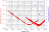 |
Fig. 12. Measured equivalent magnetic noise level (in red) and frequency response (in blue) of SCM flight model. The curves on the left are for LF antennas and the curves on the right for the MF one. The blue curves represent actually the sensors gains as a function of the frequency. |
The low noise of the MF antenna enables to observe the magnetic flux associated with the radio type III burst and the magnetic counterpart of Langmuir-like waves. The SCM dynamic performance is summarized in the Table 2.
SCM performances.
3.4. The Main Electronic Box (MEB)
The Main Electronics Box (MEB) is a stacked assembly that gathers all the electronics boards (except ANT and SCM preamplifiers) of the RPW experiment. It includes a set of radio receivers, as well as the power supply and the data processing subsystems. The combination of analyzers associated to the various electric and magnetic sensors allows to cover a wide variety of functions to explore the plasma waves in the spectral and time domain from near-DC to 16.4 MHz.
The MEB consists of the following subsystems: the nominal and redundant Low Voltage Power Supply and Power Distribution Unit (LVPS-PDU), the nominal and redundant Data Processing Unit (DPU), the biasing unit (BIAS), the Low Frequency Receiver, the Time Domain Sampler and finally the Thermal Noise and High Frequency Receiver (TNR-HFR).
Figure 13 displays the RPW frequency coverage by the above subsystems.
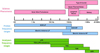 |
Fig. 13. RPW frequency coverage by its various subsystems. |
All the subsystems are assembled into a single mechanical chassis and interconnected together using harnesses, as shown in the upper panel of Fig. 14. The lower panel of this figure provides the MEB block diagram.
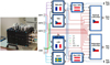 |
Fig. 14. Left: MEB mechanical chassis; right: MEB block diagram. |
The signals from sensors are amplified locally, close to ANT and SCM, and then transmitted to the MEB via dedicated harnesses and connectors. The interconnection design results from a failure analysis. The three LF components of the E-Field from ANT are passed through the BIAS unit, where they are conditioned and combined prior to be distributed to both, the LFR and TDS. The three HF components of the E-Field from ANT are routed to the TNR-HFR and then redistributed to the TDS and the LFR. Indeed, the interconnection scheme depicted above allow LFR to use the HF preamplifiers as a backup in case of failure of the DC/LF chain (partial redundancy). The three LF components of the B-Field from the SCM directly feed the LFR and TDS, while the SCM MF component feeds TDS and TNR-HFR. In addition, should LFR fail, TDS could be reconfigured in-flight in its proper LFR mode to process the ANT and SCM LF components. Finally, the LVPS-PDU and DPU are duplicated and connected as shown in Figs. 15 and 16 respectively. Both are identical but independent units, so that it is possible to activate and operate the MEB without distinction from the nominal or the redundant channel. This guarantees a complete redundancy of the vital functions in case of damage in one unit. In addition, the electrical interfaces between these units and the subsystems have been designed with the utmost care, so that failures cannot propagate from one unit to another.
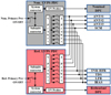 |
Fig. 15. LVPS-PDU redundancy and connections. |
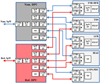 |
Fig. 16. DPU redundancy and connections. SpW stands for SpaceWire (point-to-point and full duplex communication network for S/Cs), RMAP for Remote Memory Access Protocol (additional physical layer to allow one SpaceWire node to write to and read from memory inside another SpaceWire node) and SiS for Simple Serial Interface (homemade serial point-to-point link for low data rate interfaces). |
For EMC cleanliness, the grounding scheme follows the Distributed Single Point Grounding concept, illustrated in Fig. 17. The loads (MEB subsystems and preamplifiers) are provided with isolated grounds. The latter are connected to the chassis ground on the LVPS-PDU side only.
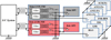 |
Fig. 17. MEB grounding scheme. |
3.4.1. The Power Supply
The RPW instrument includes two LVPS-PDU which operate in cold redundancy. The LVPS and the PDU are combined as a single unit as shown in Fig. 18.
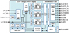 |
Fig. 18. LVPS-PDU Block diagram. |
The S/C system feeds the RPW instrument with two unregulated power lines ranging from 26 V to 29 V. In order to produce a number of isolated and well regulated power outputs to the RPW subsystems, the LVPS is built using three step-down DC-DC converters: one is devoted to the powering of the MEB system (PDU and DPU) and the two others to supply the science subsystems (see below): one to the sensitive analog parts and the other to the noisy digital parts. The converters are based on a push-pull topology with current mode control. This topology was selected with regards to the good cross regulation between output voltages and for availability of the components with low consumption in space quality. Powering during operation is realized by output common choke in fly-back mode and its voltage follows the output voltage of converters. If short circuited or overloaded, the output voltage will drop, lowering the voltage of the control circuit. This control circuit will then turn itself off and the circuit will try to start again. If the conditions that caused this power-off are resolved, the power source will restart. The feedback circuit works in current mode, controlling the duty cycle according to actual current. This allows to ease the output filtering, simplify the compensation of the feedback loop and improves the response when load steps occur. In sensitive scientific instruments of this kind, the power supply is a central element to achieve the strong EMC cleanliness requirements. As a consequence, the DC–DC power converters must operated at a unique fixed frequency, and this chopping frequency must be controlled by a crystal oscillator. This design approach allows to concentrate power-supply noise and harmonics into well known and narrow frequency bands; and providing clean spectral regions where sensitive measurements can be obtained.
The LVPS-PDU switching frequency is selected at 200 kHz. The crystal controlled design coupled with the isolation of outputs and grounds resulted in a very good self-compatibility within the RPW instrument. The power distribution function is provided by the PDU block. By the means of specific transistor switches, it distributes the supply voltages to the various RPW subsystems. Upon the reception of the appropriate commands from the DPU, the PDU can power ON or OFF any unit independently of each other. The PDU also implements overcurrent and overvoltage protections on all the secondary outputs. Once a short circuit or an overvoltage occurs, the event is detected. If it persists beyond the timeout limits, the relevant converters are shutdown. In addition, the PDU constantly monitors the secondary voltages and current consumption of all outputs. Local temperatures are also part of the PDU housekeeping stream. The LVPS-PDU achieved the worthy end-to-end efficiency of > 70%.
3.4.2. The Data Processing Unit (DPU)
The RPW instrument integrates two DPU, operating in cold redundancy. They control all the RPW operations and tasks. In particular, they handle the communication with the Data Management System (DMS) of the S/C using the two independent SpaceWire interfaces. Commands from the S/C are decoded and executed or distributed to the subsystems. On the other hand, data from the subsystems are collected, and eventually post-processed in the DPU prior to be sent to the DMS. In addition, the housekeeping data of whole the instrument are transmitted periodically.
The DPU is designed around the UT699 LEON3-FT (Fault Tolerant) processor, which is based upon the industry-standard SPARC V8 architecture. The UT699 is a 32-bit pipelined processor, that provides four SpaceWire interfaces, memory controller, and a set of peripherals communicating internally via the Advanced Microcontroller Bus Architecture backplane.
As shown in Fig. 19, the DPU is equipped with a 64 kB boot PROM (Programmable Read Only Memory), 4 MB of EEPROM (Electrically Erasable PROM) and 64 MB of radiation-hardened SRAM (Static Random Access Memory). Finally, a FPGA (Field-Programmable Gate Array) is used to support the processor communication, memory access, and to sample the local housekeeping.
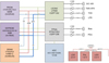 |
Fig. 19. DPU Block diagram. |
With the application of power (or by reset command or watchdog time-out), the DPUs processor boots from reliable rad-hardened PROM. Upon a dedicated command, the boot loader copies the DPU Application Software (DAS) stored in the EEPROM into the SRAM. The DAS then takes the operations control. One image of flight software is kept in the prime EEPROM bank and another version is kept in the backup location. This allows for reliable and safe operation even at times when the flight software in one EEPROM bank is being replaced by ground command. In addition to the communication link to the S/C, the DPU has three other SpaceWire links. They are used to connect the various RPW science subsystems; in the present case LFR, TDS and TNR-HFR. Two low-rate links are dedicated to communicate with the BIAS unit and the PDU. They are implemented into the FPGA using a homemade serial protocol.
3.5. The antenna biasing unit (BIAS)
The BIAS subsystem is responsible for (1) amplifying and distributing the analog signal from antennas in the LF frequency range, and (2) driving the current bias to antennas. It consists of one electronics board within the MEB and one front-end electronics part within each of the antenna preamplifiers. The analog output signal from the BIAS unit is distributed to the LFR and the TDS units (see Fig. 21). The BIAS subsystem’s functionality is controlled by one FPGA which in its turn is controlled by the DPU unit. All the BIAS software is run in the DPU.
The BIAS unit allows the current bias to each of the antennas to be set in the range −60 to +60 μA. The schematics of biasing implementation is shown in Fig. 20. By setting the appropriate bias current the antenna potential can be shifted closer to the local plasma potential. Such biased antennas allow to measure the electric field in the DC/LF frequency range with higher accuracy and lower noise level. In addition, biased antennas allow to measure the satellite potential. To assess the required biasing levels, regular current sweeps on each of the antennas are planned. The bias current calibration is performed by connecting a calibration resistor Rcal instead of the antenna as seen on Fig. 20.
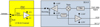 |
Fig. 20. Floating ground and current biasing concept. The floating ground has a range of ±50 V relative to the S/C structure. The transition from active current to passive bootstrapping is set to 100 Hz. This latter is much lower than the RC frequency of a biased probe, which will vary from several to several tens of kHz depending on the distance to the sun. |
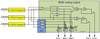 |
Fig. 21. Schematics of BIAS analog output signals that are sent to the LFR and TDS units. |
Figure 22 shows all possible measured signals that can be produced by the BIAS unit. There are four types of signals: (i) the voltage of single ended antenna reduced 17x, (ii) the voltage difference between two antennas, (iii) the voltage difference with 5x amplification and high-pass filtered at 50 Hz and finally (iv) the voltage difference with 100x times amplification, high-pass filtered at 50 Hz.
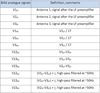 |
Fig. 22. Internal analog signals within the BIAS unit. The parameter γ can be 5 or 100. |
The higher amplification allows more sensitive electric field measurements but has accordingly reduced range. Thus, for 100x amplification assuming the effective length of the distance between two antennas to be 6 m, we have a measurement range of about ±10 mV m−1. The output from the BIAS unit can be different combination of the above described signals.
Figure 23 shows all possible configurations of the BIAS unit output signals V1BIAS ...V5BIAS. All five signals are distributed to the LFR unit, while the TDS unit receives only V1BIAS ...V3BIAS. Figure 21 shows the schematics of the BIAS unit and how the different output signals are formed. In the standard operation the output contains the single ended signal from antenna V1 and the two differentials V12 and V23, both DC and alternative current (AC). The AC signals are high-pass filtered at 50 Hz and amplified 5 or 100 times depending on the relay settings. There are several modes of output signal configuration which would be appropriate in the case of failure of some of the antennas. In addition, there are several modes for the calibration purposes.
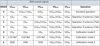 |
Fig. 23. BIAS unit output signals V1BIAS to V5BIAS in the different modes. The choice of selecting V12 or V13 for mode 0 is done using a relay and both signals are thus not accessible simultaneously in the same mode. |
3.6. Low Frequency Receiver (LFR)
The Low Frequency Receiver (LFR) is designed to digitize and process signals from the electric antennas (ANT) and the search coil magnetometer (SCM) over a frequency range of quasi DC to ∼10 kHz. Figure 24 shows the LFR overall block diagram. A wide range of time-domain and spectral-domain data products is implemented in the flight software. LFR is also responsible for producing a calibration signal to the SCM, monitoring its own temperature and the temperature of the SCM. The LFR board has furthermore a special area reserved to the SCM heater circuitry. A block diagram of LFR is shown on.
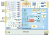 |
Fig. 24. LFR Block diagram. |
The signals measured by the three ANT voltage sensors are amplified by high- and low-frequency (LF and HF) preamplifiers. The ANT LF signals (V1LF, V2LF, V3LF) are conditioned and transformed by the BIAS board into five analog voltage signals (V1BIAS, V2BIAS, V3BIAS, V4BIAS, V5BIAS) before entering the LFR. The ANT HF signals (V1HF, V2HF, V3HF) are directly entering the LFR. Three analog voltage signals (B1LF, B2LF, B3LF) also arrive directly from the SCM LF windings. The eleven input buffers of LFR are designed to be 4th order low-pass filters with a cutoff frequency of ∼10 kHz. The input buffers for the V4BIAS and V5BIAS signals are moreover AC-coupled using a single-pole high-pass filter (−3 dB at ∼4 Hz). Eight analog signals are continuously digitized at fi = 98304 Hz through eight 14-bit ADCs (analog to digital converters). The routing strategy is based on two main configurations named BIAS_WORKS and BIAS_FAILS. Nominally, the five first ADCs are used to digitize the BIAS signals producing five data streams sampled at fi: V1_fi, V2_fi, V3_fi, V4_fi, V5_fi. In the case BIAS fails, the ANT HF signals are switched to the three first ADCs while the two next ADC inputs are switched to ground. Whatever the configuration, the three last ADCs are used to digitize the SCM signals producing three more data streams sampled at fi: B1_fi, B2_fi, B3_fi.
As illustrated on Fig. 25 and after analog-to-digital conversion, the eight data streams sampled at 98304 Hz are routinely processed within an Actel RTAX-4000D FPGA. Firstly, their cadence is reduced to f0 = 24576 Hz using an anti-aliasing and downsampling 5 second-order stages IIR filter. Then, from this stream of data sampled at f0, three other data streams sampled at f1 = 4096 Hz, f2 = 256 Hz and f3 = 16 Hz, respectively, are produced. Those sampling rates are illustrated on Fig. 1. For the generation of the f1 data stream, the f0 data stream is passed through a low-pass (5 second-order stages) IIR filter decimating by a factor 6. For the generation of the f2 and f3 data streams, decimation CIC filters, by factors 16 and 256, respectively, are previously applied to the f0 data stream before passing through the factor 6 decimation IIR filter.
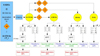 |
Fig. 25. LFR data processing. See text for more details. |
This complex data processing finally provides three kind of data products, waveforms, power spectral densities and bacic wave properties, which are detailed in Sect. 6.1.
Nominally, V1BIAS is dedicated to single-ended electric potential measurements, whereas the pairs (V2BIAS, V3BIAS) and (V4BIAS, V5BIAS) are dedicated to DC- and AC-coupled differential electric field measurements, respectively. Configurable routing parameters (R0, R1, R2) allow to select either the DC- or AC-coupled differential signals to be sampled at f0, f1 and f2 respectively, and then be processed into science data streams. For the stream of data sampled at f3 it is not configurable and only the DC-coupled pair (V2BIAS, V3BIAS) is processed. The other signals (V1BIAS, B1LF, B2LF, and B3LF) are not concerned by this restriction and are all retained in the data streams sampled at f0, f1, f2, and f3. Nevertheless, the magnetic data B1_f3, B2_f3, and B3_f3 are only optionally transmitted to S/C. Configurable modes allow some additional conditioning on the DC-coupled pair (V2BIAS, V3BIAS). This occur when BIAS operates in a non-standard mode (for instance an undesired antenna preamplifier failure): the differences V2BIAS–V1BIAS and V3BIAS–V2BIAS may digitally be performed and substituted to the stream of data just after the downsampling at f0 of the corresponding data.
3.7. Thermal Noise and High Frequency Receiver
The Thermal Noise and High Frequency Receiver (TNR-HFR or THR) consists of a wide dynamic range and high-resolution spectrometer integrating two channels in interface with the three monopoles for the electric field and the high frequency component of the magnetic search-coil.
The THR will measure the quasi-thermal Noise, the Langmuir-like waves or the solar radio bursts as described in Sect. 2. By processing cross-correlations between two channels connected to different antennas, the THR has direction-finding capabilities for tracking the solar radio bursts. Finally, the THR is also sensitive to dust impacts via the corresponding plasma cloud and pickup signal on the electric field antennas (Meyer-Vernet et al. 2009).
3.7.1. THR hardware description
The Thermal Noise Receiver (TNR) produces quasi-instantaneous spectra for the electrostatic thermal noise and/or the magnetic field in the range from 4 kHz to 1 MHz. The High Frequency Receiver (HFR) is a sweeping receiver, in the range from 500 kHz over to 16 MHz. Figure 26 shows the THR overall block diagram and Fig. 27 summarizes the THR observation frequencies, sensitivities and dynamic ranges.
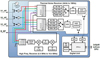 |
Fig. 26. THR block diagram. |
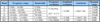 |
Fig. 27. THR observation frequencies, sensitivities and dynamic ranges. |
Because of the good amplitude resolution which is required on the whole dynamic, the receiver fits its gain according to the input level. An Automatic Gain Control (AGC) loop determines the receiver gain to a logarithmic scale as a function of the input level. This results in a normalization of the amplitude at the input of Analog to Digital (A/D) converters, and therefore a wide dynamic range. By using low noise and linear preamplifiers, the dynamic range reaches about 120 dB for the TNR range and about 80 dB for the HFR one.
The TNR frequency range is divided into four sub-bands (A, B, C and D, see Fig. 27) of 2-octaves thanks to sharp analog filters. The input signal spectral analysis is performed using a wavelets-like transform based on Finite Impulse Response digital filters. These latter are built using a Remez exchange scheme (see Elliott & Ramamohan Rao 1983 for more details). The digitized waveform of each sub-band is processed so that auto-correlations and cross-correlations are calculated for 32 log-spaced frequencies (i.e. Δf/f ∼ 4.5%), resulting on a total of 128 log-spaced frequencies for each TNR channel, as described in Sect. 6. The typical durations for the AGC stabilization are respectively 14, 3.5, 1.1 and 0.3 ms respectively for the bands A to D. Any variation of the natural signals with timescales shorter than these times will not be detected individually. The TNR provides quasi-instantaneous spectra, leading to a good spectral and temporal resolution.
The HFR is a sweeping receiver covering the frequency range from 400 kHz over to 16 MHz, as described in the next subsection. The HFR down-converts the input signals using a super-heterodyne technique. The TNR channels offer complementary signal conditioning to enhance the dynamic range. Spectra are measured simultaneously on both channels with a linear resolution. The HFR is highly programmable. Up to 324 frequencies can be selected between 0.4 and 16.4 MHz. In normal mode, the duty cycle for one frequency channel is 27 ms and the number of analyzed frequencies is 192. This yields a full HFR spectrum scan in 5.2 s.
In addition, a dedicated digital unit supports the on-board signal processing and data stream. Samples from A/D converters are successively stored into First In First Out memories and processed using a specific algorithm. The resulting auto-correlations are compressed and sent to the DPU through the serial link.
3.7.2. Real-time analysis of TNR data
In order to detect onboard the in-situ electron density, TNR-HFR detects the local plasma frequency using a simple peak detection algorithm. This algorithm is implemented by a software and works on the B, C and D bands of the TNR. The instrument will also provide the median value of the last five auto spectral components of band D, as well as the AGC value for band D. All these data will be transmitted to Earth in a low latency way (no buffering prior downloading to Earth). Scientific teams will be able to trigger a reconfiguration of the instrument(s), allowing deeper investigation of a peculiar phenomenon.
As for the LFR, the specific THR data products are described in Sect. 6.
3.8. Time Domain Sampler (TDS)
The Time Domain Sampler (TDS) subsystem of the RPW instrument is designed to capture electromagnetic waveform snapshots in the frequency range from 200 Hz to 200 kHz, resolving in particular plasma waves near electron plasma frequency and voltage spikes associated with dust impacts. The instrument digitizes analog signals from the high frequency preamplifiers of RPW antennas (V1HF, V2HF, V3HF) and the high frequency winding of the SCM search coil (BMF).
The design of TDS is shown in Fig. 28. All of the digital functionalities of TDS are implemented in Microsemi RTAX2000SL radiation hard FPGA, complemented by 16 megabytes of SRAM memory. The FPGA integrates the Leon3-FT 32-bit soft processor, spacewire interface and additional logic for signal processing. TDS analog front end electronics can be divided in two sections: low frequency and high frequency part. In nominal operation the high frequency part described here is used while the low frequency part is only used in the backup mode described in Sect. 3.8.
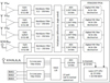 |
Fig. 28. Block diagram of TDS receiver. |
The analog front end of TDS includes a bandpass filter, band-limiting the input signal between approximately 200 Hz and 350 kHz, and a configurable gain switch allowing to increase the analog gain by 12 dB comparing to the baseline low gain setting option. This gain is set by telecommand and can be set independently for each channel. Before digitization the analog signal is routed through a multiplexer bank which allows to select which signal is digitized by each of the four analog to digital converters (ADC). For electric field measurements, the multiplexers can be used to choose between monopole antenna measurements or dipole measurements, where differential voltages between RPW antennas are sampled instead. A list of supported multiplexer configurations is given in Table 3, but in normal scientific operations it is planned to use mainly HF_SE_1 for monopole antenna measurements or HF_DIFF_1 for dipole measurements.
Nominal configuration of TDS inputs.
The high frequency analog signals are digitized by four 14-bit ADCs at a sampling frequency of 2097.1 kHz. This oversampled digital signal is afterwards downsampled in the FPGA by a factor of 4, 8, 16 or 32, after being processed by anti-aliasing FIR filters with an appropriate cutoff frequency. This decimated waveform at either 524.275 ksps, 262.138 ksps, 131.069 ksps or 65.534 sps then serves as the basis for waveform snapshots and statistical data products.
The main data product of TDS are waveform snapshots, segments of time series collected simultaneously from up to four TDS channels. The processing and selection procedure by which these snapshots are stored and sent to ground are described in Sect. 6.
3.9. TDS low frequency backup mode
TDS includes an interface to the BIAS board (only three of five channels are sampled) and to the three low frequency channels of SCM which enable TDS to operate as a limited replacement for the LFR board. This interface is only active in RPW backup mode, where TDS is switched to a dedicated LFM mode, where the nominal “high frequency” part of TDS is powered off and TDS can only sample the 6 low frequency inputs. The signals from these inputs are filtered by analog low pass anti-aliasing filters and digitized by a single 14-bit ADC feeded with a 1:8 multiplexer which cycles between the inputs in a round-robin manner, sampling each channel at 32767.2 samples per second. The data is then transmitted to ground either in the form of waveform snapshots at this sampling rate, decimated continuous waveform at a sampling rate between 1 sps and 128 sps or electromagnetic spectral matrices calculated on board.
4. RPW flight software and onboard detection of science events
4.1. The RPW flight software architecture
The RPW instrument is complex in terms of on-board software (S/W) architecture, remote monitoring and control since it embeds five different flight software which have to cooperate properly. Two flight software are located in the DPU board: the application S/W and the boot S/W. Each analyzer board (LFR, TDS, TNR-HFR) runs also its own flight software.
4.1.1. The DPU Application S/W
The DPU Application Software (called hereafter “DAS”) has been designed and built with the GERICOS framework (Plasson et al. 2016). The DAS is a sophisticated software managing various interfaces and implementing the standard ECSS PUS services (Telecommand verification, Housekeeping reporting, Event reporting, Memory management, Time management, Test connection) and also a set of services specific to the RPW experiment. The DAS interacts with all the RPW subsystems: LVPS-PDU, LFR, TDS, TNR-HFR and BIAS. It is responsible for managing the RPW modes, switching on/off the RPW sub-units, configuring and commanding the RPW sub-units, verifying and executing the RPW telecommands received from the S/C, monitoring the RPW sub-units, reporting housekeeping and events, supporting the FDIR mechanisms, distributing the time to the analyzer boards, processing, compressing (lossless compression of LFR and TDS waveforms based on the Rice compression algorithm) and packetizing the science data sent by the analyzer boards, performing science event detection. The DAS is also in charge of the BIAS sweeping procedure management. The DAS communicates with the S/C using the CCSDS (Consultative Committee for Space Data Systems) protocol over the SpaceWire network. The boot process of each analyzer flight software is performed remotely, over the SpaceWire link, by the DPU application software using the RMAP protocol which offers all the mechanisms allowing to have remote memory write and read operations highly reliable. Each analyzer board integrates an RMAP hardware controller, which allows the DPU to access to any area of its memory, including the processor registers. Thanks to this approach, the DPU can remotely configure the registers of the LEON3-FT processor analyzer boards, load the software images in the SRAM of the analyzer board and start them without intervention of any local boot software. One of the other critical features of the DAS is to continuously monitor all the RPW subsystems (currents, temperatures, heart beats, …), detect the failures, isolate them and execute autonomous recovery procedures.
4.1.2. The DPU Boot S/W
To manage the maintenance and the boot of the DPU application software, a standard and well proven architecture based on the use of a separate boot software has been implemented. The DPU boot software is a critical and low complexity software stored in PROM. The DPU application software, that is stored in the DPU EEPROM, is loaded in the working memory and started upon the reception of a dedicated TC packet by the boot software. The boot software implements also the memory management PUS service and is able to patch or fully change in EEPROM the application software.
4.1.3. LFR, THR and TDS Flight S/W
The main role of the analyzer flight software is to acquire and pre-process the raw data provided by the sensors. The pre-processing includes event detection, data reduction, data selection and lossy compression of spectral products. The communication protocol used between the DPU and the analyzers for exchanging telecommunication (TC) packets and telemetry (TM) packets is the CCSDS protocol.
4.2. The RPW software science modes
Figure 29 shows the RPW science modes and the authorized mode transitions.
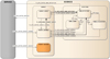 |
Fig. 29. RPW science modes. |
4.2.1. SURVEY mode
The SURVEY mode is a very simple and robust working mode in which all the data acquired from the analyzers (TDS, TNR-HFR, LFR) are entirely and continuously transferred to the S/C as scientific telemetry packets without any selection or detection from the DPU. In the SURVEY mode, the only treatments performed on data by the DPU are compression and packetization. The compression algorithm can be enabled or disabled thanks to a telecommand. The SURVEY mode is itself broken down in a SURVEY_NORMAL sub-mode (low cadence), a SURVEY_BURST sub-mode (high cadence) and a SURVEY_BACKUP sub-mode (degraded mode in which TDS replaces LFR). In the SURVEY_NORMAL sub-mode, the data rate from the analyzers is lower than 10 kbps (Kilobits per second) and the scientific TM data rate produced by the DPU is lower than 10 kbps. From an operational point of view, the activation of the SURVEY_BURST sub-mode for a given period is activated thanks to time tagged TC. Typically, the SURVEY_BURST sub-mode will be activated 10 min per day. The SURVEY_BACKUP sub-mode allows to manage the RPW degraded mode in which LFR is switched off and TDS replaces it by using its LFM mode (LFR backup mode).
4.2.2. DETECTION mode
The DETECTION mode is a complex mode in which all the data are acquired from the analyzers (TDS, TNR-HFR, LFR) at a high cadence. Detection algorithms are activated at DPU level to perform the measurements of specific Selected Burst Modes (SBMs). There are two kinds of SBM events: interplanetary shocks crossings (SBM1) and in-situ type III (SBM2). They are described below. The data are not entirely or directly transferred in TM packets at this high cadence. The DPU continuously produces a TM stream corresponding to the NORMAL mode data flow, but the high resolution data are only transmitted to the S/C Solid State Mass Memory (SSMM) if an SBM event has been detected. In the DETECTION mode, the RPW DPU interacts with other Solar Orbiter instruments such as the MAG, the Solar Wind Analyzer (SWA) or the Energetic Particles Detector (EPD). The DPU uses their data to detect the events and it sends to them periodically the S/C potential and sporadically a trigger flag if an event has been detected. The DETECTION mode is itself broken down in three sub-modes: SBM_DETECTION sub-mode, SBM1_DUMP sub-mode and SBM2_ACQUISITION sub-mode. The SBM_DETECTION sub-mode is the main sub-mode of the DETECTION mode in which the detection algorithms (SBM1 and SBM2) are activated. The acquisition and storage in a circular buffer of the SBM1 data are performed in this mode. In the SBM_DETECTION sub-mode, the LFR and TDS analyzers are put in SBM1 mode (TNR-HFR remains in NORMAL mode): they acquire data at very high rate and transmit to the DPU two data streams: a low cadence stream corresponding to the NORMAL mode data flow, lower than 10 kbps, which is compressed, packetized and transmitted directly to the S/C SSMM, and a high cadence stream corresponding to the configuration of SBM1 mode, typically 478 kbps, which is stored by the DPU in a large circular buffer (SRAM).
SBM1 detection algorithm. The SBM1 detection algorithm is based on the real-time joint analysis of the magnetic field vector provided by the MAG instrument (Horbury et al. 2020) and the proton number density and bulk velocity provided by the SWA instrument (Owen et al. 2020). This algorithm, described in details in Kruparova et al. (2012), basically detects combined temporal jumps of the magnetic field intensity and proton densities. It provides a quality factor proportional to a weighted average of the above jumps. A more technical description of the SBM1 detection algorithm is provided in Maksimovic et al. (2015). The RPW instrument enters the SBM1_DUMP sub-mode if the DPU has detected an SBM1 event. In this sub-mode, the DPU transfers the content of the SBM1 data circular buffer to the S/C SSMM: the SBM1 data packets are routed to a dedicated S/C SSMM packet store whose content is only downlinked on demand. In addition the shock detection flag from RPW is shared on-board with the other in-situ instrument (Walsh et al. 2020). The typical duration of an SBM1 event is 13 min.
SBM2 detection algorithm. The SBM2 detection algorithm is based on the real-time analysis of the electron flux provided by the EPD instrument (Rodríguez-Pacheco et al. 2020). When the fluxes of electrons measured in-situ in the range 45−145 keV and flowing in the anti-sunward direction exceeds a given threshold then the algorithm checks whether local langmuir waves are produced locally and detected by TDS. If this is the case then the RPW instrument enters the SBM2_ACQUISITION sub-mode for all the receivers. The acquisition and storage in a dedicated S/C SSMM packet store of the SBM2 data are performed only if an increase of the Langmuir waves activity has been reported by TDS in its statistics. A more detailed and technical description of the SBM2 detection algorithm is provided in Maksimovic et al. (2015). The typical duration of an SBM2 event is 120 min.
When the DAS stores an SBM event (SBM1 or SBM2) in the S/C SSMM, it sends to the ground a TM packet containing the features of the SBM event (type, quality factor, start time, duration, etc.). Thanks to these SBM features reported by the DAS, the RPW Operation Center is able to know what are the SBM events stored in the S/C SSMM (type, location, volume, etc.) and then to maintain a “map” of the SBM events stored in the S/C SSMM. The total number of SBM events which can be stored on the S/C SSMM will vary during the course of the mission since it depends on the ability of the SSMM to download its data to ground. The specification has been that, in standard conditions, RPW should have the possibility to store up to 42 SBM1 events and 4 SBM2 events.
4.2.3. BURST mode
In addition to SURVEY and DETECTION modes RPW can run in burst mode and produce, given the allocated average telemetry of 5000 kbps, about 10 min per day of burst data. These latter will consist of both spectral data at high temporal cadence and waveform data with high sampling rate. The precise strategy for these scheduled burst modes will be coordinated with the other in-situ instrument (Walsh et al. 2020).
5. RPW operations
Following the general Solar Orbiter science objectives (Müller et al. 2020), the RPW team has to provide calibrated data to the scientific community three months after the raw telemetry has been received on ground. The RPW Operations Center (ROC), located at the Laboratoire d’Etudes Spatiales et d’Instrumentation en Astrophysique (LESIA) in Meudon, France, is in charge of the RPW ground segment activities. It has the three following main tasks: (i) monitor the Science capabilities of the instrument, (ii) prepare the RPW operations and science configurations and (iii) produce the RPW calibrated data.
The RPW operations and data production will be performed in close connection with the Solar Orbiter Operations Center (SOC) located in the European Space Astronomy Center near Madrid, Spain. The SOC structure is described in Sanchez et al. (in prep.).
5.1. Concept of operations
Depending of the science objectives and operational constraints, RPW can be operated with a set of pre-defined instrument configurations. In the nominal case RPW is tuned into the SBM_DETECTION sub-mode with a “default science” configuration. When RPW enters in the SBM_DETECTION sub-mode, SBM events can be automatically detected and the resulting high cadence data saved on a specific packet store on-board, as described in the previous section. When appropriate and when the ROC has received the green light from the SOC, the RPW team decides, using the SBM event map, the event quality factors computed and assigned on-board, and the analysis of the MAG, SWA & EPD low latency data which SBM event shall be downlinked. Depending of the telemetry bit rate and the data downlink priority, retrieving on-ground all the packet data of a selected SBM event can take between few days and few weeks. Additionally, at least few minutes per day will be dedicated to acquire data in the high cadence SURVEY_BURST sub-mode. The triggering time and duration of the RPW SURVEY_BURST sub-mode windows are planned in coordination with other in situ instruments, which have their own “burst” modes. A description of the existing instrument configurations is available online1. New configurations can be implemented by the RPW team during the mission if needed.
The Solar Orbiter science operations planning starts at the beginning of the cruise phase (Zouganelis et al. 2020). RPW then continuously acquires science data 24 h a day with the three other in situ instruments on-board the S/C. The remote-sensing payload is only switched-on during specific “remote-sensing windows”. The selective downlink of the SBM event data stored on-board is planned to be tested during the cruise phase and be fully operational for the nominal phase. During the latter the ROC submits instrument commands to the SOC every week. In parallel to the instrument configuration setting, the ROC ensures routine operations on-board, i.e., subsystem calibrations, BIAS unit current sweeping and tuning.
5.2. RPW Operations Center overview
The instrument operations are driven by the ROC, from the instructions of the RPW Operations Board (ROB). The mission level planning for every orbit (6 months) is discussed within the Solar Orbiter Science Operations Working Group, in agreement with the Solar Orbiter Science Working Team.
In order to ensure its activity during the mission, the ROC relies on a dedicated infrastructure at LESIA. Especially, Web interfaces are accessible to the ROB in order to view and prepare the operations planning for RPW, as well as select the SBM event data to downlink. Specific applications are used by ROC operators to generate and submit the instrument operation requests to the SOC. Data visualization tools allows ROC and RPW teams to monitor the science performance of the instrument and verify the command execution. The prime monitoring of the RPW systems is ensured by the Solar Obiter Mission Operations Centre (MOC), located at the European Space Operations Centre (ESOC) in Darmstadt, Germany.
Additionally LESIA also maintains a suite of Software Ground Support Equipement (SGSE) with the aims of: (i) maximizing the instrument science data return, i.e., increasing the accumulated telemetry data volume and optimizing the detection rate of the on-board SBM algorithms, (ii) testing the command execution on-ground, (iii) supporting investigations in case of anomalies detected on-board.
6. RPW data products
Three main types of data products will be available from RPW for scientific use: (i) electric and Magnetic waveforms at various sampling frequencies and with various duration, (ii) power Spectral Densities for both Electric and Magnetic signals at various sampling frequencies and with various duration and (iii) electric and Magnetic cross products and related waves polarization and propagation properties.
Each of the three subsystems, LFR, THR and TDS, will provide their own products which at the end will be stored in different daily files. RPW and all its subsystems are expected to run continuously during the whole science phase of the mission.
The detailed data files and products descriptions together with the corresponding user manuals are available online2. Below we describe briefly for each subsystem how the data are processed on-board and their content.
6.1. LFR Data products
For the first three frequency channels (digitized signals at f0, f1 and f2 as illustrated on Fig. 25) different kinds of data are produced and transmitted to DPU: waveforms (WFs), averaged spectral matrices (ASMs) and waves basic parameters (BPs). For the last one (digitazed signals at f3) only WFs are produced and transmitted. Depending on the RPW working mode and the frequency channel, the WFs are captured continuously or periodically (regularly spaced 2048-point snapshots). For the NORMAL, SBM2 or BURST, and SBM1 modes (see Sect. 4), the WFs at f3, f2 and f1, respectively, are continuously transmitted to DPU. In addition, for the NORMAL mode, 2048 data points snapshots of WF at f0, f1 and f2, centered with respect of each other, are recorded every 300 s.
The ASMs are produced routinely on-board, nominally every 4 s, with two electric and three magnetic field components corresponding to 5 × 5 electromagnetic spectral matrices. Their components are calculated as auto and cross power spectra averaged over 4 s using a 256-point Fast Fourier Transform, with a Hann window applied. For the frequency channels f2, f1 and f0, 96, 104, and 88 linearly spaced frequency bins, with frequency resolutions of 1 Hz, 16 Hz and 96 Hz, respectively, are retained in order to cover the frequency range from 6.5 Hz to 10 032 Hz with small overlap. Nominally, the ASMs are transmitted to DPU at a very low rate: just one 4 s ASM every 3600 s, in order to verify that the BPs are computed properly.
The BPs are designed to bring the best time coverage of the wave data. The basic parameters are indeed just wave parameters computed on-board from the ASMs, minimizing the amount of data to be transmitted. These wave parameters are wave polarization properties, k-vector characterizations or the sunward component of the Poynting vector. Before computation of the BPs, the frequency resolutions of the ASMs are reduced by averaging over packets of 8 (nominal mode) or 4 (burst modes) consecutive bins. A frequency mask can be applied at this step in order to filter out spurious bins. The BPs are divided into two sets, BP1s and BP2s, the first set being transmitted with a full time coverage, the second set with time gaps. The BP1s consist of seven spectral quantities which aim at characterizing the waves. Five of them can be calculated without difficulties: the total electric and magnetic power spectra, the wave normal vector and a wave ellipticity estimator (Means 1972), and a wave planarity estimator (Samson & Olson 1980). The two others necessitate onboard cross-calibration between the electric and magnetic sensors: the radial-component of the Poynting vector, and a phase velocity estimator (based on the Maxwell–Faraday equation). This on-board cross-calibration will be done by updating into the LFR flight software a proper calibration table from ground by specific telecomands. The BP2s are just a compression of the frequency averaged ASMs: the ten cross spectral components of the matrices are normalized using the Schwarz inequality and the five auto spectral components are stored using a binary logarithmic compression. Nominally, the BP1s and BP2s are computed for the three frequency channels where the WFs are not transmitted continuously (i.e., for f2, f1 and f0) and are transmitted to DPU every 4 s and 20 s, respectively. For the SBM2 or BURST modes, they are computed for the f1 and f0 channels, and transmitted every 1 s and 5 s, respectively. For the SBM1 mode, they are computed for the f0 channel and transmitted every 0.25 s and 1 s.
6.2. THR Data products
The THR produces continuously auto-spectra and cross-spectra on a regular cadence. These spectral products are recorded over commandable time periods which can last from 1.13 s to 12 s for the TNR and from 2 s to 22 s for the HFR. The latter integration times sets also to temporal resolution for the THR data which, in normal operation, will typically be on the order of 10 to 20 s on orbit, depending on the telemetry allocation for the THR. The Normal mode configuration, summarized by Fig. 30 will be two channel measurements allowing both quasi-thermal noise and radio direction finding (DF) measurements. The direction finding is a technique that determines the direction and the angular size of a radio source. In the case of Solar Orbiter, which is a non spinning S/C, techniques described by Krupar et al. (2012) will be used.
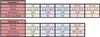 |
Fig. 30. Temporal sequence for TNR-HFR normal mode measurements. This sequence is meant mostly for the QTN and the solar radio science objectives. |
As illustrated in Fig. 30, in normal mode with no magnetic measurements from the SCM bi-band antenna, three consecutive TNR full frequency scans (the four bands A, B, C & D) are firstly performed on each of the two receivers channels connected to different antennas. These three scans will be used for the radio DF. The total number of frequencies for the auto-spectra (power) measurements is 128 (32 per band). For the cross-products (real and imaginary parts) only 96 frequencies will be available, since there is no direction finding in band A which correspond to frequencies too low compared to the expected local plasma frequency. Once the DF is performed, the TNR will remain connected to channel one and perform two full frequency scans in dipole mode (V1 − V2 and V2 − V3) for the Quasi thermal noise, while the HFR will be connected in dipole to channel two in order to perform a full high frequency scan for Solar radio measurements. Many other more complex science modes, involving also magnetic measurements from the SCM bi-band antenna, are possible. They will be described in a specific user manual are available online3 at the time of the release of the RPW public data by ESA.
As for the burst modes, there will be no specific configurations for the THR since these receivers are basically limited by the minimum integration time necessary for their radio measurements. Note however that in SBM2 the THR will be connected to the medium frequency SCM measurements, at the expenses of direction finding which will not be useful in this case.
6.3. TDS Data products and on-board processing
The main data product of TDS are waveform snapshots, segments of time series collected simultaneously from up to four TDS channels. The length of the snapshots is configurable and can be any power of 2 between 1024 samples and 65536 samples. There are two categories of waveform snapshots. Regular snapshots are taken periodically at pre-defined times and in normal RPW operation these are taken simultaneously with LFR waveform snapshots. Triggered snapshots, on the other hand, are selected based on their content. The on-board software evaluates one snapshot taken every second and assigns each snapshot a quality factor using a selected triggering algorithm. The snapshots with the highest quality are retained in TDS memory and dumped to DPU after a predefined interval (6 h for normal mode snapshots, 5 min in SBM2 mode). There are separate queues of normal mode and SBM2 mode triggered snapshots and each can hold up to 6 megabytes of data (up to 48 snapshots of 16384 samples).
The baseline algorithm used in TDS assigns the quality factor based on the snapshot peak amplitude, a ratio of peak amplitude to median of the signal, and bandwidth of the main spectral peak identified in the Fourier spectrum calculated from the snapshot. This algorithm efficiently distinguishes between coherent waves, such as Langmuir waves, characterized by a narrow bandwidth and small peak to median ratio, and isolated voltage spikes associated with impacts of dust, which results in a very large peak to median ratio and wide bandwidth. Other algorithms for the quality factor calculation can be configured, such as the selection based on peak or rms snapshot amplitude. The outputs of the processing algorithms are used to calculate on-board statistics of the observed signals and these are transmitted in the form of average values and histograms. The parameters that can be included in the statistics include peak and rms amplitude of snapshots and of identified waves, wave frequency, a number of identified waves and dust spikes, and the amplitude and width of identified dust spikes. Furthermore, TDS can produce a continuous waveform of maximum absolute value of raw observed signals at 2097.1 kHz, where the maxima are taken over 7.8 ms (or a multiple of this interval). This product is nominally only enabled in BURST mode. A summary of TDS data products in nominal mode is shown in Table 4.
TDS data products in nominal mode of operation.
6.4. Data processing pipeline
RPW raw telemetry data available in the Solar Obiter MOC Data Dissemination System (DDS) are requested by the ROC every day. The ROC then produces within 48 h a first preliminary version of RPW uncalibrated (L1) and calibrated (L2) science data. These preliminary data are only distributed to the RPW consortium and external partners, that is other in-situ instrument PI teams and SOC. The ROC delivers the definitive RPW science data within three months to the Solar Orbiter Archive of the European Space Astronomy Centre (ESAC) science data centre (Sanchez et al., in prep.) near Madrid in Spain.
The production and delivery of the so-called low latency data as well as the mission ancillary data, i.e., orbit, attitude, reference frame, on-board time to UTC conversion, are under the responsibility of the SOC.
7. Summary
The RPW instrument will measure the magnetic and electric fields, plasma wave spectra and polarization properties, the S/C floating potential, and solar radio emissions in the interplanetary medium. All these measurements are absolutely crucial in order to fulfill the science objectives of the Solar Orbiter mission. Table 5 summarizes the main capabilities of the instrument.
Summary of the RPW capabilities.
At the time of submitting this article, we have carried out all the tests to demonstrate that performances of the instrument are compliant with the initial requirements. These test and assessments are described in details in Maksimovic (2019) where the pre-launch performances of the whole instrument are described. We are confident that once launched RPW will fulfill its science objectives and provide excellent data.
Acknowledgments
We thank the Centre National d’Etudes Spatiales (CNES, French space agency), the Centre National de Recherches Scientifiques (CNRS), the Paris Observatory, The Swedish National Space Agency, ESA-PRODEX and all the involved institutes for their funding. We thank the ESA Solar Orbiter project team and the Aibus Defense and Space technical team. Javier Rodriguez-Pacheco wishes to thank FEDER/MCIU-AEI/Project ESP2017-88436-R. Several people have been involved in the genesis, development and completion of the RPW instrument. We wish to thank Kader Amsif, Thierry Battault, Jean-Michel Benezeth, Pierre Bodin, Louis Bougeret, Clément Brysbaert, Jerome Carron, Fabienne Casoli, Hélène Combes, Christoper Cuomo, Gonzalo Campos Garrido, Rodolphe Clédassou, Nicolas Doumas, Pascal Durand, Delphine Faye, A. Gaget, Philippe Gasc, Stanislas Guillemant, Christian Imbert, Philippe Laget, Yann Le Huede, Nicolas Liquières, Filippo Marliani, Stéphane Mary, Samuel Mellé, Johan Panh, Denis Payan, Jean-Yves Prado, Christian Puillet, Desi Raulin, E. Revert, Amandine Ribaimont, Guillaume Rioland, Denis Schwander, Jean-Michel Travert, Sylvain Trémolières, Mathieu Worgague.
References
- Alexandrova, O., Saur, J., Lacombe, C., et al. 2009, Phys. Rev. Lett., 103, 165003 [NASA ADS] [CrossRef] [Google Scholar]
- Alexandrova, O., Chen, C. H. K., Sorriso-Valvo, L., Horbury, T. S., & Bale, S. D. 2013, Space Sci. Rev., 178, 101 [NASA ADS] [CrossRef] [Google Scholar]
- Alexandrova, O., Krishna Jagarlamudi, V., Rossi, C., et al. 2020, Nat. Comm., submitted [arXiv:2004.01102] [Google Scholar]
- Bale, S. D., Reiner, M. J., Bougeret, J.-L., et al. 1999, Geophys. Res. Lett., 26, 1573 [NASA ADS] [CrossRef] [Google Scholar]
- Bougeret, J.-L., Kaiser, M. L., Kellogg, P. J., et al. 1995, Space Sci. Rev., 71, 231 [NASA ADS] [CrossRef] [Google Scholar]
- Bruno, R., & Carbone, V. 2013, Liv. Rev. Sol. Phys., 10, 2 [Google Scholar]
- Bruno, R., Carbone, V., Bavassano, B., & Sorriso-Valvo, L. 2005, Adv. Space Res., 35, 939 [CrossRef] [Google Scholar]
- Chen, X., Kontar, E. P., Yu, S., et al. 2018, ApJ, 856, 73 [CrossRef] [Google Scholar]
- Dehmel, G., Neubauer, F. M., Lukoschus, D., Wawretzko, J., & Lammers, E. 1975, Raumfahrtforschung, 19, 241 [Google Scholar]
- Elliott, D. F., & Ramamohan Rao, K. 1983, The Solar Probe Plus Mission: Humanity’s First Visit to Our Star (Elsevier) [Google Scholar]
- Fox, N. J., Velli, M. C., Bale, S. D., et al. 2016, Space Sci. Rev., 204, 7 [NASA ADS] [CrossRef] [Google Scholar]
- García-Marirrodriga, C., Pacros, A., Strandmoe, S., et al. 2020, A&A, in press, https://doi.org/10.1051/0004-6361/202038519 (Solar Orbiter SI) [Google Scholar]
- Greco, A., Matthaeus, W. H., Servidio, S., Chuychai, P., & Dmitruk, P. 2009, ApJ, 691, L111 [NASA ADS] [CrossRef] [Google Scholar]
- Hellinger, P., Trávníček, P., Kasper, J. C., & Lazarus, A. J. 2006, Geophys. Res. Lett., 33, L09101 [NASA ADS] [CrossRef] [Google Scholar]
- Horbury, T. S., O’Brien, H., Carrasco Blazquez, I., et al. 2020, A&A, 642, A9 (Solar Orbiter SI) [NASA ADS] [CrossRef] [EDP Sciences] [Google Scholar]
- Kontar, E. P., Yu, S., Kuznetsov, A. A., et al. 2017, Nat. Commun., 8, 1515 [NASA ADS] [CrossRef] [Google Scholar]
- Krupar, V., Santolik, O., Cecconi, B., et al. 2012, J. Geophys. Res. (Space Phys.), 117, A06101 [CrossRef] [Google Scholar]
- Krupar, V., Maksimovic, M., Kontar, E. P., et al. 2018, ApJ, 857, 82 [NASA ADS] [CrossRef] [Google Scholar]
- Kruparova, O., Maksimovic, M., Safrankova, J., Nemecek, Z., & Santolik, O. 2012, AGU Fall Meeting Abstracts, SH41B-2114 [Google Scholar]
- Lefeuvre, F., Blanc, E., Pinçon, J.-L., et al. 2008, Space Sci. Rev., 137, 301 [CrossRef] [Google Scholar]
- Lin, R. P., Potter, D. W., Gurnett, D. A., & Scarf, F. L. 1981, ApJ, 251, 364 [NASA ADS] [CrossRef] [Google Scholar]
- Lion, S., Alexandrova, O., & Zaslavsky, A. 2016, ApJ, 824, 47 [NASA ADS] [CrossRef] [Google Scholar]
- Maksimovic, M. 2019, RPW-SYS-SOW-001518-LES – RPW Science Performances, https://rpw.lesia.obspm.fr/ [Google Scholar]
- Maksimovic, M., Hoang, S., Meyer-Vernet, N., et al. 1995, J. Geophys. Res., 100, 19881 [CrossRef] [Google Scholar]
- Maksimovic, M., Bougeret, J.-L., Perche, C., et al. 1998, Geophys. Res. Lett., 25, 1265 [CrossRef] [Google Scholar]
- Maksimovic, M., Issautier, K., Bale, S. D., et al. 2001, Adv. Space Sci., 493, 285 [Google Scholar]
- Maksimovic, M., Krupar, V., & Alexandrova, O. 2015, RPW-SCI-NTT-000243-LES – RPW Instrument: Definition of the In-Flight Burst Modes Detection Algorithms, https://rpw.lesia.obspm.fr/ [Google Scholar]
- Maruca, B. A., Kasper, J. C., & Gary, S. P. 2012, ApJ, 748, 137 [NASA ADS] [CrossRef] [Google Scholar]
- Matteini, L., Landi, S., Hellinger, P., et al. 2007, Geophys. Res. Lett., 34, 20105 [NASA ADS] [CrossRef] [Google Scholar]
- Matteini, L., Hellinger, P., Landi, S., Trávníček, P. M., & Velli, M. 2012, Space Sci. Rev., 172, 373 [NASA ADS] [CrossRef] [Google Scholar]
- Means, J. D. 1972, J. Geophys. Res. (1896–1977), 77, 5551 [CrossRef] [Google Scholar]
- Melrose, D. B. 1982, Sol. Phys., 79, 173 [NASA ADS] [CrossRef] [Google Scholar]
- Meyer-Vernet, N., Maksimovic, M., Czechowski, A., et al. 2009, Sol. Phys., 256, 463 [NASA ADS] [CrossRef] [Google Scholar]
- Meyer-Vernet, N., Issautier, K., & Moncuquet, M. 2017, J. Geophys. Res., 122, 7925 [CrossRef] [Google Scholar]
- Müller, D., St Cyr, O. C., Zouganelis, I., et al. 2020, A&A, 642, A1 (Solar Orbiter SI) [CrossRef] [EDP Sciences] [Google Scholar]
- Owen, C. J., Bruno, R., Livi, S., et al. 2020, A&A, 642, A16 (Solar Orbiter SI) [EDP Sciences] [Google Scholar]
- Plasson, P., Cuomo, C., Gabriel, G., et al. 2016, Proc. of the Data Systems in Aerospace Conference (DASIA), Tallin, Estonia, 2016. European Space Agency, (Special Publication) ESA SP, SP-736 [Google Scholar]
- Rodríguez-Pacheco, J., Wimmer-Schweingruber, R. F., Mason, G. M., et al. 2020, A&A, 642, A7 (Solar Orbiter SI) [CrossRef] [EDP Sciences] [Google Scholar]
- Samson, J. C., & Olson, J. V. 1980, Geophys. J., 61, 115 [CrossRef] [Google Scholar]
- Sharykin, I. N., Kontar, E. P., & Kuznetsov, A. A. 2018, Sol. Phys., 293, 115 [NASA ADS] [CrossRef] [Google Scholar]
- Sperveslage, K., Neubauer, F. M., Baumgärtel, K., & Ness, N. F. 2000, Nonlinear Process. Geophys., 7, 191 [NASA ADS] [CrossRef] [Google Scholar]
- Štverák, Š., Trávníček, P., Maksimovic, M., et al. 2008, J. Geophys. Res., 113, 3103 [Google Scholar]
- Thejappa, G., & MacDowall, R. J. 2008, ApJ, 676, 1338 [NASA ADS] [CrossRef] [Google Scholar]
- Tsurutani, B. T., Lakhina, G. S., Verkhoglyadova, O. P., et al. 2011, J. Geophys. Res. (Space Phys.), 116, A02103 [Google Scholar]
- Walsh, A. P., Horbury, T. S., Maksimovic, M., et al. 2020, A&A, 642, A5 (Solar Orbiter SI) [CrossRef] [EDP Sciences] [Google Scholar]
- Zouganelis, I., De Groof, A., Walsh, A. P., et al. 2020, A&A, 642, A3 (Solar Orbiter SI) [CrossRef] [EDP Sciences] [Google Scholar]
All Tables
All Figures
|
Fig. 1. Variations with Heliocentric distance of the characteristic plasma frequencies. Are also indicated the instrument various sampling frequencies (see Sect. 3.4 for more details). |
| In the text | |
|
Fig. 2. Various natural phenomena that will be observed by the RPW instrument in the DC–LF frequency range and associated sensitivity and dynamical range requirements. The spectral breaks are assumed to occur at proton and electron gyro-frequencies (see text for more details). |
| In the text | |
|
Fig. 3. Various natural phenomena that will be observed by the RPW instrument in the radio domain and associated sensitivity and dynamical range requirements (see text for more details). As far as the QTN is concerned one can note that because we will be in a regime where the antenna length is comparable to the Debye length, the plasma peaks are not prominent and do not appear visible on this figure. |
| In the text | |
|
Fig. 4. Magnetic field fluctuations of various natural phenomena that will be observed by the RPW instrument and associated sensitivity and dynamical range requirements. The spectral breaks are assumed to occur at proton and electron gyro-frequencies (see text for more details). |
| In the text | |
|
Fig. 5. Payload accommodation on Solar Orbiter S/C. The RPW sub-units are indicated in red. The electric Antenna system (ANT) consists of a set of three identical antennas deployed from +Z axis (Antenna PZ) and from the opposite corners of the S/C +Y and -Y walls (Antennas PY and MY). The SCM consists of a set of three magnetic antennas mounted orthogonally. Their orientations, in the S/C reference frame, are given by the three vectors in the upper left part of the figure. Finally the Main Electronic Box (MEB) is located inside the S/C body. |
| In the text | |
|
Fig. 6. From top to bottom: antenna overview in stowed configuration. Antenna dimensions one deployed. Main dimensions of the deployed stacers (in meter) with the conductive part of the sensor indicated in blue. |
| In the text | |
|
Fig. 7. Three antenna units dimensions and configurations once deployed. |
| In the text | |
|
Fig. 8. Antenna preamplifiers electrical design. See text for more details. |
| In the text | |
|
Fig. 9. Antenna radio-electrical properties. |
| In the text | |
|
Fig. 10. Various contributions to the antenna stray capacitance. We note that Va′ is the measured voltage while Va is the natural voltage in the plasma. |
| In the text | |
|
Fig. 11. Flight model of the search-coil magnetometer. |
| In the text | |
|
Fig. 12. Measured equivalent magnetic noise level (in red) and frequency response (in blue) of SCM flight model. The curves on the left are for LF antennas and the curves on the right for the MF one. The blue curves represent actually the sensors gains as a function of the frequency. |
| In the text | |
|
Fig. 13. RPW frequency coverage by its various subsystems. |
| In the text | |
|
Fig. 14. Left: MEB mechanical chassis; right: MEB block diagram. |
| In the text | |
|
Fig. 15. LVPS-PDU redundancy and connections. |
| In the text | |
|
Fig. 16. DPU redundancy and connections. SpW stands for SpaceWire (point-to-point and full duplex communication network for S/Cs), RMAP for Remote Memory Access Protocol (additional physical layer to allow one SpaceWire node to write to and read from memory inside another SpaceWire node) and SiS for Simple Serial Interface (homemade serial point-to-point link for low data rate interfaces). |
| In the text | |
|
Fig. 17. MEB grounding scheme. |
| In the text | |
|
Fig. 18. LVPS-PDU Block diagram. |
| In the text | |
|
Fig. 19. DPU Block diagram. |
| In the text | |
|
Fig. 20. Floating ground and current biasing concept. The floating ground has a range of ±50 V relative to the S/C structure. The transition from active current to passive bootstrapping is set to 100 Hz. This latter is much lower than the RC frequency of a biased probe, which will vary from several to several tens of kHz depending on the distance to the sun. |
| In the text | |
|
Fig. 21. Schematics of BIAS analog output signals that are sent to the LFR and TDS units. |
| In the text | |
|
Fig. 22. Internal analog signals within the BIAS unit. The parameter γ can be 5 or 100. |
| In the text | |
|
Fig. 23. BIAS unit output signals V1BIAS to V5BIAS in the different modes. The choice of selecting V12 or V13 for mode 0 is done using a relay and both signals are thus not accessible simultaneously in the same mode. |
| In the text | |
|
Fig. 24. LFR Block diagram. |
| In the text | |
|
Fig. 25. LFR data processing. See text for more details. |
| In the text | |
|
Fig. 26. THR block diagram. |
| In the text | |
|
Fig. 27. THR observation frequencies, sensitivities and dynamic ranges. |
| In the text | |
|
Fig. 28. Block diagram of TDS receiver. |
| In the text | |
|
Fig. 29. RPW science modes. |
| In the text | |
|
Fig. 30. Temporal sequence for TNR-HFR normal mode measurements. This sequence is meant mostly for the QTN and the solar radio science objectives. |
| In the text | |
Current usage metrics show cumulative count of Article Views (full-text article views including HTML views, PDF and ePub downloads, according to the available data) and Abstracts Views on Vision4Press platform.
Data correspond to usage on the plateform after 2015. The current usage metrics is available 48-96 hours after online publication and is updated daily on week days.
Initial download of the metrics may take a while.