| Issue |
A&A
Volume 699, July 2025
|
|
|---|---|---|
| Article Number | A120 | |
| Number of page(s) | 15 | |
| Section | Stellar structure and evolution | |
| DOI | https://doi.org/10.1051/0004-6361/202554727 | |
| Published online | 02 July 2025 | |
High angular resolution near-ultraviolet polarization imaging of the Herbig Ae/Be star LK-Hα-233
Université de Strasbourg, CNRS, Observatoire astronomique de Strasbourg, UMR 7550, F-67000 Strasbourg, France
⋆ Corresponding author: This email address is being protected from spambots. You need JavaScript enabled to view it.
Received:
24
March
2025
Accepted:
20
May
2025
Abstract
Context. Herbig Ae/Be stars are young, pre-main-sequence stars that provide critical insights into the processes of stellar formation, early stellar evolution, and protoplanetary disks.
Aims. Two key features of such stars are their circumstellar dusty disk and bipolar ionized outflows, which are critical components for understanding planet formation processes and the deposition of energy and/or matter in the interstellar medium, respectively. In this context, imaging polarimetry is arguably the most precise tool for characterizing the various structures and dynamics around the central star, due to the sensitivity of polarization to the morphology of the emitting, scattering, and absorbing media.
Methods. We used previously unpublished, near-ultraviolet polarimetric data of LK-Hα-233 taken by the Faint Object Camera aboard the Hubble Space Telescope in 1991, 1994 and 1995, which remained archived despite their quality. Using the most recent and robust reduction pipeline for this instrument, we obtained high spatial resolution (0.0287 × 0.0287 arcsecond2) maps of this object at 4118 Å, together with polarimetric measurements.
Results. A dark lane, bisecting the approaching and receding polar outflows, suggests the presence of a circumstellar disk or dust torus, which obscures the pre-main-sequence star and collimates the ejecta. Polarization reveals that the outflows have an X-shaped structure with a significant centrosymmetric pattern in the polarization angle, indicating that the outflows are both hollow and scatter the emission from the buried star. We constrain the half-opening angle of both the outflows and the circumstellar disk, determine the inclination of the system, and estimate the obscured star’s intrinsic flux.
Conclusions. This study highlights the importance of high-resolution polarimetric observations in understanding the complex environment around Herbig Ae/Be stars and advocates for future similar instruments.
Key words: polarization / scattering / techniques: polarimetric / circumstellar matter / stars: individual: LK-Halpha-233 / stars: pre-main sequence
© The Authors 2025
 Open Access article, published by EDP Sciences, under the terms of the Creative Commons Attribution License (https://creativecommons.org/licenses/by/4.0), which permits unrestricted use, distribution, and reproduction in any medium, provided the original work is properly cited.
This article is published in open access under the Subscribe to Open model. This email address is being protected from spambots. You need JavaScript enabled to view it. to support open access publication.
1. Introduction
The Faint Object Camera (FOC) aboard the Hubble Space Telescope (HST) was a pivotal instrument in astronomical research, known for its high-angular-resolution imaging and polarimetric capabilities (Macchetto 1982; Nota 1996). Operating in the 1150–6500 Å wavelength range, the FOC utilized a combination of advanced optics and detectors to achieve unprecedented spatial resolution (14 × 14 arcseconds2 field of view with pixel dimensions as small as 0.01435 × 0.01435 arcseconds2), crucial for resolving fine structures in distant astronomical objects. Its ability to perform polarimetry allowed astronomers to measure the polarization of light, providing insights into the scattering mechanisms and magnetic fields within various astrophysical environments. The high angular resolution of the FOC, combined with its polarimetric functionality, made it an exceptionally powerful diagnostic tool for studying complex systems, such as gravitational lenses (Nguyen et al. 1999), active galactic nuclei (AGNs, Capetti et al. 1995; Thomson et al. 1995; Kishimoto et al. 2002), supernovae (Sparks et al. 1999), and other intricate cosmic phenomena. These capabilities enabled detailed investigations into the morphology and dynamics of celestial objects until the instrument was removed during the fourth servicing mission (SM3B) in March 2002.
Among the sources observed by the HST/FOC, AGNs are the most numerous, followed by supernovae and a few other singular objects. Among them is LK-Hα-233. This source was part of a calibration proposal, so it is not included in the catalog of sources observed for scientific purposes. Its observation was therefore forgotten and was never analyzed in a scientific context. LK-Hα-233 is not the only source to have been consigned to oblivion in the archives, as illustrated by the project undertaken by Barnouin et al. (2023). However, their work focuses on AGNs. In this paper, we focus on the only Herbig Ae/Be star ever observed by the FOC.
Herbig Ae/Be stars are a subclass of pre-main-sequence stars that occupy a crucial phase in the evolutionary timeline of stellar development. These young, intermediate-mass stars, with masses ranging between 1.5 and 10 solar masses (Vioque et al. 2018; Brittain et al. 2023), are characterized by their strong emission lines (Manoj et al. 2006), infrared excesses (Hartmann et al. 1993), and associations with reflection nebulae (Herbig 1960; Neckel et al. 1987). Discovered and classified by George Herbig in the 1960s (Herbig 1960), these stars serve as prime laboratories for studying the processes of star formation and early stellar evolution.
The defining features of Herbig Ae/Be stars include their surrounding protoplanetary disks and the presence of bipolar jets and outflows (Hillenbrand et al. 1992). These circumstellar disks, composed of gas and dust, are the birthplaces of planetary systems, making Herbig Ae/Be stars critical to understanding the mechanisms of planet formation (Brittain et al. 2023). The interaction between the star and its disk leads to complex phenomena such as accretion, disk winds, and the formation of circumstellar structures, all of which can be studied through multiwavelength observations. For example, the Near-Infrared Camera and Multi Object Spectrometer (NICMOS) on the HST provided the first resolved scattered light images of dusty disks around pre-main-sequence stars (Weinberger et al. 1999) ; the Atacama Large Millimeter/submillimeter Array (ALMA) can spatially resolve the disk emission in several Herbig Ae/Be stars due to significant advances in spatial resolution (about 0.05–0.1 arcseconds; Andrews et al. 2018); and the Gaia satellite, operating in the optical band, makes it possible to homogeneously determine the masses, ages, luminosities, distances, photometric variabilities, and infrared excesses of large samples of Herbig Ae/Be stars (Vioque et al. 2018). Polarimetry has also been used effectively to study these stars, from determining the dust composition in the disks (Murakawa 2010b) to constraining the accretion processes and linking them to T Tauri stars, which are the lower-mass counterparts to Herbig Ae/Be stars (Vink 2015; Ababakr et al. 2017).
The star of interest in this study, LK-Hα-233, has been included in many of these studies. Located at a distance of 880 pc (Testi et al. 1998; Manoj et al. 2006), where 1 arcsec corresponds to 0.0042664 pc, 0.0139151 ly, or 880 au, it has always been a good target for imaging and polarimetry. Aspin et al. (1985), using imaging polarimetry and photometry in three broad bands (B, V, R) discovered that the central star is hidden behind a large obscuring region and that the associated faint nebulosity seen in the optical (Herbig 1960) is, in fact, a highly polarized, bipolar outflow, suggesting scattering from an optically thin medium. This discovery was confirmed by near-infrared speckle interferometry (Leinert et al. 1993), as well as by HST’s Space Telescope Imaging Spectrograph (STIS) and Wide Field Planetary Camera (WFPC2) observations (Melnikov et al. 2008). These authors also reported the presence of a dark lane, caused either by a circumstellar disk or a dust torus that obscures the star itself, and helped characterize the bipolar outflows.
In this paper, we explore what the previously overlooked near-ultraviolet polarimetric data from the FOC can reveal about the circumstellar environment of LK-Hα-233. In Sect. 2, we describe how the data were retrieved and reduced and present the three different observations made with the FOC. In Sect. 3, we analyze in detail the spatially resolved polarization of LK-Hα-233 and derive constraints on the outflows and circumstellar disk geometry. We discuss our results in Sect. 4 and draw a connection between the general geometry of Herbig Ae/Be stars and AGNs. We conclude in Sect. 5, highlighting the need for future high-angular-resolution polarimeters to study protoplanetary disks and stellar evolution.
2. The forgotten archives
Originally, the principal investigators of these archival observations, Francesco Paresce and Philip Hodge, aimed to determine the FOC unpolarized transmission coefficients in orbit to a relative accuracy of 0.3% by observing a standard, extended, unpolarized (< 0.15%) source (NGC 5272), and to determine the effective polarimeter position angle offset and polarized transmission coefficients to a relative accuracy of 3% by observing a standard polarized source (LK-Hα-233) through the blue polarizers. The LK-Hα-233 observations were analyzed in an instrumental context, but never in a scientific context, and have remained dormant in the archives ever since. We also verified that no other similar objects had been overlooked, and we confirm that this is the only unpublished, never-analyzed observation of a pre-main-sequence star with the HST/FOC.
2.1. Data reduction
Three LK-Hα-233 observations were made using the FOC aboard the HST: one in 1991, another in 1994, and the last in 1995. For all observations, the f/96 mode was used (512 × 512 pixel format) without zoom, offering a spatial resolution of 0.01435 × 0.01435 arcseconds2 per pixel, equivalent to an effective resolution of 6.116 × 10⁻⁵ pc (≈12.6 AU) for a 7 × 7 arcseconds field of view. However, the final effective spatial resolution is limited by binning and smoothing, and thus is slightly degraded (see next paragraph). Exposures were taken with the F430W broadband blue filter, centered on 3960 Å (bandpass 870 Å), along with three polarizing Rochon prisms (POL0, POL60, and POL120). In contrast to, for example, the HST/FOC observation of M87 (Marin et al. 2024a), no FOC warming up, preliminary shots were taken to precisely place the source on the same detector region, nor internal flats to remove reseau marks that were used to calibrate geometrical distortion of the cathode ray tube. This is important in the analysis of the results.
To reduce the data downloaded from the MAST HST Legacy Archive1, we followed the guidelines and used the automated, generalized reduction pipeline presented in Barnouin et al. (2023). A detailed technical description can be found in this paper and others in this series (Barnouin et al. 2024, Marin et al. 2024a). Only the parametrization used to obtain the fully reduced polarization maps is described here. After downloading the data, the raw POL0, POL60, and POL120 images were cropped to show the same region of interest. Background estimation was performed by analyzing the intensity histogram of each image using the Freedman-Diaconis sampling rule. A Gaussian fit was applied to the histogram, with the mean value representing the background level. The images were aligned with a precision of approximately 0.1 pixels, then binned at the Nyquist frequency, that is, 2 × 2 pixels. The Nyquist–Shannon theorem states that an analog signal can be digitized without aliasing error only when the sampling rate is greater than or at least twice the highest frequency component in a given signal (Shannon 1949). This allows us to maximize the spatial resolution of the map while retaining reliable spatial and polarization information. The images were then smoothed using a Gaussian kernel with a full width at a half-maximum of 2 pixels, twice the size of a resampled pixel. For each pixel, the Stokes parameters I, Q, and U (and their associated uncertainties) were computed, along with the debiased polarization degree P, and the electric vector position angle θ. The final maps were rotated so that north is up (θ = 0°), with rotation of θ following the IAU convention (the electric vector position angle of polarization is measured from north and increases toward east). No deconvolution was applied during the process. The resulting images have a spatial resolution of 0.0287 arcseconds (≈25.2 AU), which makes them the highest angular resolution polarimetric maps of this object to date-almost ten times more resolved than the total flux HST/STIS and HST/WFPC2 observations presented in Melnikov et al. (2008).
However, as we discuss in the following subsections, this high spatial resolution requires a high photon count to obtain statistically credible polarization measurements in each individual pixel. More polarimetric information can be obtained using maps with slightly lower spatial resolution to maximize the counts in each pixel, and thus detect the polarization of LK-Hα-233 with greater certainty. Therefore, the high-resolution images shown below are accompanied by medium-resolution images, where a spatial binning of 0.1 arcseconds has been performed, with a Gaussian smoothing of 0.2 arcseconds. All other reduction details are the same between the high- and medium-resolution final images. Full-scale images are presented in the appendix for better visibility.
2.2. The 1991 observation
The first observation (Program ID: 3873) was taken between November 20 and November 22, 1991. Each polarizer accumulated approximately 3.0 ks, resulting in a total exposure time of about 2.5 hours in polarimetric mode. This observation is notable for having been acquired when the HST still had spherical aberration in its primary mirror. This flaw caused the mirror to be too flat by approximately 2.2 μm at its edges, leading to blurred and distorted images (White & Hanisch 1991).
Despite this defect, we present the 1991 observed polarization maps of LK-Hα-233 in Fig. 1. The maps show the color-coded total flux, spatially sampled at the Nyquist frequency (left) and at 0.1 arcsecond per pixel (right). Polarization information is overplotted on the flux using vectors whose length is proportional to P and whose orientation traces θ. Due to the large spatial resolution of the map, the vectors are barely visible, but full-scale images are presented in the appendix. We find that LK-Hα-233 has an almost isotropic flux distribution, with a slight elongation in the northeast to southwest direction (position angle ≈66°, in agreement with the value of 60–70° found by Corcoran & Ray 1998). More than 50% of the observed flux comes from the inner subarcsecond region. A network of gray dots appears in the source flux; these correspond to the instrument’s reseau markings, which could not be corrected due to the absence of prior internal flats. These points are often associated with polarization vectors that are only observational artifacts. No polarization vector intrinsic to the source is reported in the high-resolution image, but a centrosymmetric polarization pattern is clearly visible in the medium-resolution map. This polarization pattern will be analyzed in detail in Sect. 3.
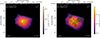 |
Fig. 1. Left: 1991 pre-COSTAR HST/FOC observation of LK-Hα-233 resampled according to the Nyquist–Shannon sampling theorem (i.e., 2 × 2 pixels2 or 0.0287 × 0.0287 arcseconds2), to ensure individual pixels yield meaningfully polarization measurements. The total flux is color-coded and expressed in units of erg cm−2 s−1 Å−1. Polarization vectors are displayed for [S/N]P ≥ 3, although at this spatial resolution they are difficult to resolve visually (larger images are presented in the appendices). Total flux contours are displayed for 0.8%, 2%, 5%, 10%, 20%, and 50% of the maximum flux. In the top-left corner, we indicate the total flux F, polarization degree P, and polarization angle θ values, integrated over the whole field of view (7 × 7 arcseconds2 in this image). Following the IAU convention, north is up and the polarization angle positively rotates toward the east. Right: Same image but with a spatial binning of 0.1 arcsecond per pixel. The polarization pattern highlighted by the vectors becomes more apparent at this scale. |
The source presents an integrated (7 × 7 arcseconds2) total flux of ∼1.6 × 10⁻¹⁴ erg cm−2 s−1 Å−1. It is difficult to assess the validity of this flux measurement as no continuum values are reported in the literature at this waveband or in the optical. However, the integrated polarization, 11.1% ± 0.2% at 150.9° ± 0.4°, is entirely consistent with the values reported by Vrba et al. (1979), i.e., 10.8% ± 0.1% at 153.9° ± 0.2° in the B band with a 10 arcsecond aperture. We note that this polarization angle is perpendicular to the position angle of the outflows, likely indicating perpendicular scattering from stellar photons onto the ejecta. Thus, it appears that HST aberration, despite blurring the details of the observed source, does not significantly distort the measured polarization values (as demonstrated by the observation of the active galactic nucleus NGC 1068 before and after correction of the aberration; see Capetti et al. 1995).
2.3. The 1994 observation
The second observation (Program ID: 5522) was taken on November 1, 1994. Each polarizer accumulated approximately 1.5 ks, resulting in a total exposure time of about 1.2 hours in polarimetric mode. This observation, as well as the one obtained in 1995, benefits from the installation of the Corrective Optics Space Telescope Axial Replacement (COSTAR) in 1993 during a servicing mission. This corrective system was designed to compensate for the primary mirror’s flaw by deploying small, precisely shaped mirrors into the optical paths of several of Hubble’s scientific instruments, such as the FOC. These corrective mirrors redirected and refocused light to eliminate spherical aberration (Hartig et al. 1993).
The 1994 observation of LK-Hα-233 is presented in Fig. 2. The increase in sharpness is striking. The source is now resolved into distinct components, even though the pointing was slightly inaccurate. The source appears in the bottom-left corner of the FOC field of view and is partially cut off. Nevertheless, the central and western components of the source, the star and the approaching blue-shifted outflow (see Melnikov et al. 2008), respectively, are clearly visible. The position angle of the outflows is confirmed at 66° ± 1°. A rectilinear zone of weaker flux now clearly separates the eastern and western winds, which spread in a conical fashion from their apex (the unresolved pre-main-sequence star). We also observe several polarization vectors that are clearly distinct from the reseau marks, indicating that [S/N]P ≥ 3 polarized pixels are detected. The medium-resolution image also shows the centrosymmetric polarization pattern, but with a greater number of pixels where polarization is clearly measured compared to the distorted 1991 image. The flux, polarization degree, and polarization angle reported on the medium-resolution image appear to differ somewhat from those of the high-resolution map. This effect is due to the binning and smoothing applied to the Stokes Q, U, and I parameters prior to computing the polarization. This processing step alters the local vector structure (particularly in regions with steep polarization gradients or low signal) by averaging the Stokes parameters over larger areas, which can lead to a reduction in polarization degree and shifts in polarization angle, even though the underlying physical signal remains the same. The same applies to the 1995 observation, but not to the 1991 pointing, as the lack of COSTAR corrections had already blurred the image.
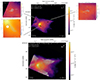 |
Fig. 2. Same as Fig. 1 but for the 1994 post-COSTAR HST/FOC observation of LK-Hα-233. The top panel shows the high-resolution map, with inserts indicating where [S/N]P ≥ 3 polarization vectors are detected. The white dot corresponds to a reseau mark that was masked during the reduction process. The bottom panel shows the medium-resolution map. Due to slightly incorrect pointing, the source appears in the bottom-left corner of the FOC field of view and is partially cut off. The improved image sharpness resulting from the COSTAR corrective optics package is clearly visible. |
From the high-resolution image, where the smoothing is minimal and therefore only slightly affects regions near the edge of the field of view, the integrated flux is ∼1.4 × 10⁻¹⁴ erg cm−2 s−1 Å−1. It is marginally lower than in 1991, but the fact that a fraction of the source has been cut off must be considered. Flux variation is not unusual for Herbig Ae/be stars, as such objects are known to vary both in both continuum and line fluxes (Perez et al. 1993; Mendigutía et al. 2011). We also note that the observed integrated polarization is 4.9% ± 0.2% at 131.8° ± 1.0°. The polarization degree and angle are very different from the integrated value measured in 1991 (although they remain perpendicular to the outflows), which is also expected for a Herbig Ae/be star. Indeed, Jain & Bhatt (1995) have demonstrated that polarimetric variability is a common feature of this class of objects, with variability spanning months to years. However, caution must be exercised with this apparent variability of polarization, since part of the source extends beyond the field of view of the instrument, something that can alter the integrated polarization measurement.
2.4. The 1995 observation
The third and final observation (Program ID: 5522, same as the second observation) was taken between June 17 and June 18, 1995. Each polarizer accumulated approximately 1.5 ks, resulting in a total exposure time of about 1.2 hours in polarimetric mode.
The 1995 observation of LK-Hα-233 is presented in Fig. 3. The pointing accuracy was better, but, again, a fraction of the source is cut off. In this instance, only the extremity of the western wind is cut, which should not hinder the analysis, unlike the 1994 observation, where a much larger fraction of the object was outside of the field of view. The source presents similar flux geometry and intensity, as highlighted by the flux contours in Figs. 2 and 3.
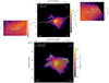 |
Fig. 3. Same as Fig. 2 but for the 1995 post-COSTAR HST/FOC observation of LK-Hα-233. Due to a minor pointing offset, the western extremity of the source falls partially outside the field of view. |
The integrated flux is ∼1.2 × 10⁻¹⁴ erg cm−2 s−1 Å−1, slightly lower than in the 1994 observation. The observed integrated polarization is 12.7% ± 0.2% at 163.7° ± 0.5°. The polarization again differs from the 1991 and 1994 values, but the polarization angle remains oriented perpendicular to the ejecta. Over the three epochs, the polarization exhibits variability, but this is less certain for the total flux.
3. A deeper analysis of the data
3.1. A polarized view
We begin by examining the 1995 HST/FOC image in polarized flux (the product of total flux F and polarization degree P) in Fig. 4, which can be compared with the corresponding image in total flux (Fig. 3). Polarized flux maps are known to provide sharper contrast than total flux images, where part of the emission is scattered by diffuse material along the line of sight or near the object of interest. The polarized flux has the advantage of removing this environmental flux, allowing better focus on the emitting, scattering, and absorbing regions associated with the source itself.
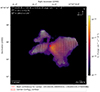 |
Fig. 4. Medium-resolution polarized flux map from the 1995 post-COSTAR HST/FOC observation of LK-Hα-233. The red cross marks the estimated location of the hidden star. |
The polarization vectors superimposed on the images reveal regions of high polarization (reaching more than 50% in many pixels) that do not correlate with the peak of total flux emission. In contrast, although the peak flux (F)is observed at the apex of the outflows, high degrees of polarization are measured at the extremities of the biconical outflows. However, the degree of polarization is not uniform at the end or within the winds but appears to be maximal only at the outer edges of the conical winds, leaving the center of the winds relatively unpolarized. Such an X-shaped structure provides compelling evidence for the hollowness of the envelope, as suggested in previous studies for young stellar objects (Caratti o Garatti et al. 2016), protostars (Lee et al. 2022), and even AGNs (Elvis 2000).
Notably, a region at the base of the oppositely directed outflows exhibits significantly lower polarization compared to the outflows. This creates a rectilinear zone about 0.25 arcseconds wide, which corresponds precisely to the position of the minimum flux observed in total flux (see Fig. 3, although this zone is only 0.1 arcseconds wide in total flux). These observations suggest that the inner region of LK-Hα-233 is obscured, likely by circumstellar material. This dark lane, visible in both polarization and total flux, is consistent with the presence of a circumstellar disk or a dust torus, as postulated by Melnikov et al. (2008). No polarization vectors are associated with the dark lane, indicating that few, if any, photons directly escape through the dusty circumnuclear obscurer toward us. The optical depth of the dark lane is therefore larger than unity (e.g., the simulations from Murakawa 2010a and Marin et al. 2012).
Another clear aspect of the polarized flux map is that it reveals a structure that is somewhat narrower than in the total flux map, with sharper contours for the bipolar ejecta. LK-Hα-233 truly resembles a butterfly in polarized flux: the geometry of the outflows is precisely revealed, together with the central region where obscuration occurs. The conical structure of the wind, apparently launched from a compact region, is well defined. Its half-opening angles with respect to the central axis of the winds are approximately 44° and 50° for the western (blueshifted) and eastern (redshifted) outflows, respectively. In turn, assuming that the outflows fill the solid angle left by the obscuring protoplanetary dusty disk, this constrains the disk half-opening angle to about 40–46° with respect to the disk midplane.
3.2. Locating the central star
We find that the polarization of LK-Hα-233 exhibits a centrosymmetric pattern (see the medium resolution Figs. A.2, A.4, and A.6), a result already established with single-epoch and lower spatial resolution observations, such as the 0.5 arcsec polarization maps of Aspin et al. (1985). The overall distribution of the polarization vectors closely resembles the point-source scattering case, which can be used to precisely determine the position of the emission source, even if it is obscured by a thick veil of dust and gas. When a photon undergoes single scattering from a point source onto an ionized polar outflow, the resulting polarization has an electric vector position angle perpendicular to the direction of the source. Taking into account the full uncertainties in the measured polarization angle of pixels with [S/N]P ≥ 5, and under the assumption of single scattering onto an ionized medium within a single plane, we derive the location of the hidden emission source following the procedure detailed in Kishimoto (1999) and Barnouin et al. (2024).Marin et al. (2023) also present a similar use of this technique to the Galactic center.
The deduced location of the star in LK-Hα-233 is shown in Fig. 4, using the 1995 observations, i.e., the less cropped of the two post-COSTAR pointings. The location of the hidden star, whose coordinates are indicated in the figure, is precisely at the base of the western outflow, near the brightest flux patches seen in total and polarized fluxes, at the edge of the dark lane that bisects the Herbig Ae star. The fact that the star is not closer to the plane of the dark lane indicated that the inclination of the entire structure is less than 90° (i.e., perpendicularity).
3.3. Aperture-dependent polarimetry
Having determined the location of the hidden star, we simulated a circular aperture onto the 1995 map, centered on the star, and increased its radius to examine how the polarization of the system evolves. Expanding the aperture helps to determine how different regions of the system contribute to the overall polarization signal and potentially reveals distinct scattering regions. As the aperture grows, variations in polarization degree and angle may indicate the presence of multiple scattering structures that affect the light from the hidden star.
The results of this exercise are presented in Fig. 5. Focusing first on the total flux (top panel), we find that with increasing aperture radius, the amount of photons detected steeply rises within the first 0.5 arcsecond around the hidden star. This is expected since the dark lane is only 0.25 arcseconds wide. Scattering at the base of the outflows then allows radiation to escape via perpendicular scattering, which strongly increases the observed total flux. For large apertures, the flux appears to plateau at a value of approximately 1.2 × 10⁻¹⁴ erg cm−2 s−1 Å−1, which is the value measured for the full field of view. Notably, the polarization degree (Fig. 5, middle panel) shows a modest value of about 8% within the first 0.25 arcseconds around the hidden star, then increases to more than 11% at 0.5 arcseconds. Beyond this radius, the degree of polarization continues to increase with distance from the center of the object, where single diffusion is most effective in producing a high degree of polarization. This behavior is also evident in the angle of the polarization position, which rotates gradually as the aperture radius increases. It begins at approximately 140° and reaches around 165° at the largest apertures. When comparing these polarization angles to the outflow position angle (60–70° as reported by Corcoran & Ray 1998, or 66° ± 1° as derived in this study), we find that the polarization vectors are approximately perpendicular to the outflow direction across all apertures. However, a median deviation of approximately 16° with respect to orthogonality could indicate that the dust disk might be slightly misaligned with respect to the biconical outflows.
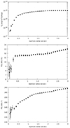 |
Fig. 5. Variation of the total flux (top), polarization degree (middle), and polarization angle (bottom) as a function of increasing aperture radius, centered on the location of the hidden star. Error bars are shown, but may be too small to be visible. |
3.4. Scanning the various polarized regions
The various maps shown in this study clearly show that both the total and polarized fluxes are spatially variable across LK-Hα-233. To explore its complexity in greater detail, we divided the 1995 map into five regions, covering most of the source. Each region is defined by a synthetic circular aperture with a radius of 1 arcsecond (see Fig. 6), labeled as follows: region 1 (the core), region 2 (upper extremity of the eastern outflow), region 3 (lower extremity of the eastern outflow), region 4 (lower extremity of the western outflow), and region 5 (upper extremity of the western outflow). The integrated flux and polarization for each region are listed in Table 1.
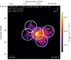 |
Fig. 6. The five distinct regions of LK-Hα-233 detected for detailed analysis. The map is the 1995 observation (identical to Fig. 3). Each white circle corresponds to an aperture with a radius of 1 arcsecond. |
Individually, the different regions exhibit distinct characteristics. Region 1 concentrates most of the source flux (∼8.2 × 10⁻¹⁵ ergs cm−2 s−1 Å−1, see Table 1), as discussed in Sect. 2 and dominates the values of P and θ in larger fields of view. This is expected, as it corresponds to the base of the bipolar winds, where the near-ultraviolet emission from the western component is maximal and where spatially dependent polarization (0–20%) is detected, resulting in high polarized fluxes (see Fig. A.6). The relatively low value of P (∼11%) at the peak of the total flux may be due to two distinct, yet compatible, reasons. On the one hand, this could result from photons scattering multiple times before escaping, as expected near the highest-density regions (Murakawa 2010b). This would naturally explain the increase in polarization observed farther out in the bipolar nebula as single scattering becomes dominant. On the other hand, it may indicate that the base of the outflow is dynamically active, with many interacting cloudlets or filaments of ionized matter, gas, and dust, resulting in canceling polarization vectors at spatial scales below the resolution of our HST/FOC maps. A polarimetric map with finer spatial resolution would help to distinguish the dominant mechanism.
Region 2, the upper extremity of the eastern outflow, is more than an order of magnitude fainter in flux than region 1 (the core). In contrast, P is significantly higher at this location, where the ejected medium is likely less perturbed than in the core, and where single scattering in an optically thinner medium would naturally result in less depolarization (Melnikov et al. 2008). Region 3, the lower extremity of the eastern outflow, also shows a dim flux. The integrated polarization degree is remarkably high, exceeding 52%, again suggesting an optically thin medium that is outflowing without strong internal perturbations, reinforcing the validity of the hypothesis used in Sect. 3.2 to estimate the position of the obscured star. Region 4, the lower extremity of the western outflow, is moderately bright (∼1.3 × 10⁻¹⁵ ergs cm−2 s−1 Å−1) and its polarization is slightly higher than in the core region (region 1). Finally, region 5, the upper extremity of the western outflow, exhibits both moderate brightness (∼1.4 × 10⁻¹⁵ ergs cm−2 s−1 Å−1) and a high polarization degree (∼38%). For these four regions, the observed polarization angle remains perpendicular to the symmetry axis of the system, once their deviation from the central axis of the winds is taken into account.
3.5. Variability of the polarization
As previously mentioned in Sect. 2.3, Herbig Ae/Be stars are known to vary both in total flux and polarization, with timescales ranging from months to years (Perez et al. 1993; Jain & Bhatt 1995; Mendigutía et al. 2011). Jain & Bhatt (1995), in particular, noted that “variations in the polarization position angle are not always correlated with variations in the degree of polarization”. Waters & Waelkens (1998) also reported that “variations in polarization are often correlated with deep photometric minima, and they can be explained in terms of dense dust clouds obscuring the light from the star and allowing only light scattered by dust particles to escape.” Having reduced and analyzed both the complete images and different subregions in the three polarimetric datasets, we now examine the intrinsic variability of the source in greater detail.
Figure 7 presents the integrated total flux (top left), polarized flux (bottom left), polarization degree (top right), and polarization angle (bottom right) for the total field of view of the HST/FOC observations, as well as for the five regions defined and examined in Sect. 3.4. For the full field of view, the integration was performed over 7 × 7 arcsecond windows, while for the five subregions, the integration windows had a radius of 1 arcsecond. Due to the pointing error that resulted in part of the object being cut off in 1994, data for some points are unavailable in the 1994 observation (regions 2, 3, and 4).
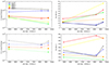 |
Fig. 7. Variability of LK-Hα-233 in total flux (top left), polarized flux (bottom left), polarization degree (top right), and polarization angle (bottom right) as a function of time (in modified Julian date). We accounted for the three HST/FOC observations; however, due to a pointing error which cut off part of the object in 1994, some data points are unavailable from that epoch. Except for the black crosses (full field of view, 7 × 7 arcseconds), all other points correspond to 1 arcsecond aperture radius integration windows at the five different regions presented in Fig. 6. Error bars are shown but may be too small to be visible. |
We find that the variability of LK-Hα-233 is more complex than previously anticipated:
-
For the entire object integrated over the full field of view, the total flux marginally decreases with time, whereas the polarized flux shows a stronger decrease from 1991 to 1994, followed by an increase in the final epoch. This behavior is driven by variations in the polarization, with P reaching its lowest value lowest in 1994. Such variation in the polarization degree is associated with a rotation of the polarization position angle. Although this appears to contradict the findings of Jain & Bhatt (1995), it should be noted that the 1994 and 1995 observations are cropped, and therefore values should be interpreted with caution.
-
The temporal behavior of the central region (region 1) closely follows that of the complete field of view, except for the total flux, which increases from 1991 to 1995, then decreases. The polarization degree is again minimal in 1994 and is associated with a rotation of the polarization angle. As a result, the behavior of the full field of view image appears to be constrained by the core region and, despite the Herbig Ae/Be system being cropped out, remains reliable. In this region, variations in the polarization position angle are correlated with variations in the degree of polarization.
-
Region 2 (upper extremity of the eastern outflow) has only two points, but the global trend from 1991 to 1995 is a decrease in both total and polarized flux, accompanied by a steep rise in polarization (from 12.3% ± 0.4% to 32.0% ± 1.3%) and a ∼7° rotation of the polarization angle.
-
Region 3 (lower extremity of the eastern outflow) also has two points, but their temporal behavior differs from that of region 2: the total flux decreases with time, but the polarized flux increases. The rise in P is even stronger than in region 2 (from 12.6% ± 0.4% to 51.2% ± 1.0%) and the rotation of the polarization angle is about 28°.
-
Region 4 (lower extremity of the western outflow) also has two points and behaves similarly to region 2, with comparable changes in polarization degree and angle, although the increase in P is slightly greater (six percentage points between the two observations).
-
Finally, region 5 (upper extremity of the western outflow) has three points and exhibits a distinct trend: its total flux decreases between 1991 and 1995 and then increases in 1995. The polarized flux of region 5 follows the same trend, with a continuous increase in P over three years. However, in contrast to the other regions with sufficient data, the polarization position angle in region 5 rotates with a different sign compared to the full field of view and region 1: the polarization angles increase by +20° between 1991 and 1995, then decrease by approximately −9°.
Our multiepoch polarimetric observations of LK-Hα-233 reveal complex spatial and temporal variability in both total and polarized flux. Although global trends are largely governed by the central region, the outflows exhibit distinct polarization behavior, suggesting asymmetries in dust distribution and scattering processes. The observed changes in polarization degree and position angle indicate evolving circumstellar structures, possibly linked to variable dust obscuration or disk reconfiguration (Waters & Waelkens 1998; Marin & Schartmann 2017). Observing Herbig Ae/Be stars at high spatial resolution is therefore essential to disentangle and quantify the contribution of the central object from the large-scale outflows.
4. Discussion
4.1. The inclination of the system
Using the data collected during this analysis, we have constrained the geometry of both the accretion disk (flared, half-opening angle of 40–46° with respect to the disk midplane) and of the outflows (biconical, hollow, collimated by the circumstellar dust, half-opening angle of 44–50° with respect to the central axis of the winds). The outflows scatter the obscured starlight toward us and we can use this information to estimate, at first order, the inclination of the entire system.
In the idealized case where scattering occurs on free electrons and no significant unpolarized (diluting) component is present, the linear polarization degree P can be approximated by the classical equation for Thomson scattering: P = (1 − μ2)/(1 + μ2), where μ = cos θ and θ is the scattering angle (Kishimoto 1999). This expression derives from the ratio of the Stokes parameters: the numerator corresponds to the polarized intensity (Stokes Q and U), and the denominator to the total intensity (Stokes I). It assumes that the scattered light originates from a compact illuminating source such that the scattering volume subtended by each image pixel occupies a small solid angle as seen from the source. It also assumes single scattering and a low optical depth medium. The core region of the system is dominated by multiple scattering in a dense environment, so we cannot rely on polarimetric measurements from this spatial location. However, we can use the polarization measured at the extremities of the winds as a proxy to calculate the inclination of the object, since single scattering appears to dominate at these locations (see Sect. 3.3).
On our polarization maps from all three epochs, we measure a polarization degree that ranges from 60 to 80% at the ends of the winds, within a 0.5 arcsecond circular aperture. This translates into an inclination of 60–70°. Although this is a rough estimate, it is consistent with the values obtained by Perrin et al. (2009), who estimated that the disk is inclined by 65° ± 5° relative to the plane of the sky using numerical radiative transfer disk models. In contrast, Bastien & Menard (1990), also using radiative transfer models, determined an inclination of 85–90°. Because we observe the eastern, opposite outflow (redshifted; see Melnikov et al. 2008) and do not observe the central pre-main-sequence star, the system must have an inclination greater than the disk half-opening angle, so that our line of sight is intercepted by dust. Therefore, even if we cannot be certain of the global inclination of the system, we can still derive a strict upper limit to the inclination of the source, which must have an orientation below the half-opening angle of the disk, i.e., ≥45° relative to the plane of the sky.
To highlight the significance of determining the system’s orientation, we estimate which fraction of the stellar flux is represented by the measured fluxes resulting from scattering in the polar winds, using the inclination constraints we derived. Based on the numerical work of Marin et al. (2012), in which a central, isotropic, compact illuminating source of optical radiation is surrounded by an optically thick, dusty disk that only allows an electron-filled wind to escape along the polar (unobstructed) direction-a geometry that mimics very well the case of Herbig Ae/be star systems-we can provide a reasonable estimate. From their Fig. 19 (bottom panel), an inclination larger than 45° implies that only 1–10% of the original flux is scattered toward the observer, depending on the exact inclination of the system. This suggests that the intrinsic flux of LK-Hα-233 is at least 10–100 times greater than 10−14 ergs cm−2 s−1 Å−1. This estimate assumes that electron scattering dominates polarigenic opacity in the wind. However, if dust scattering dominates (as seems to be the case for this object, see Vrba et al. 1979; Aspin et al. 1985 and Leinert et al. 1993), Goosmann & Gaskell (2007) showed that the observed flux under such conditions may represent only ∼0.1% of the intrinsic emission. In that case, the true stellar flux could be up to 1000 times higher than observed, implying an intrinsic flux closer to a few times 10−11 ergs cm−2 s−1 Å−1 at 4118 Å.
4.2. How are the winds created?
We find that the winds of LK-Hα-233 are hollow, brighter in total flux at the wind base but stronger in polarization at the wind’s maximal extension. The geometry of the ejecta, revealed in polarized flux, forms an X shape. Its half-opening angle is 44–50° with respect to the central axis of the winds. Scattering prevails in the winds, as shown by the centrosymmetric pattern of the polarization vectors. These particularities can help constrain the ejection mechanism at work here.
Although the specific mechanisms of wind launching and collimation differ, disk-born winds (e.g., Ustyugova et al. 1995), X-winds originating near the disk–magnetosphere boundary (e.g., Romanova et al. 2009), and stellar winds from open magnetic field lines anchored to the star’s surface (e.g., Decampli 1981) can produce hollow winds, but their ranges of half-opening angles differ. Disk winds launch from a range of radii on the accretion disk, resulting in a wide-angle outflow. The exact angle depends on the strength and configuration of the magnetic field, the accretion rate, and the specific disk properties, but the typical range of values spans 6°–60° (Blandford & Payne 1982; Pudritz et al. 2007), with most of the mass flux occurring in a conical shell with half-opening angle of 25°–30° (De Villiers et al. 2005). In the case of X-winds, because they originate near the disk-magnetosphere boundary, they are thought to be more tightly collimated compared to disk-born winds. The strong magnetic fields in this region help to focus the wind into a narrower cone of half-opening angles, typically ranging from 10° to 30° (Shu et al. 1994; Lovelace et al. 2014). Finally, stellar winds launched from the magnetic poles of the star can be highly collimated, especially if the magnetic field lines are well ordered and strong. However, if the magnetic field is weaker or more chaotic, the winds can have a broader opening angle, typically ranging from 10° to 40° (Shore 1987). With a measured half-opening angle between 44° and 50°, our analysis favors disk-born winds. However, it should be noted that each model can reproduce these values with the right set of (sometimes extreme) parameters. Therefore, the opening angle alone is insufficient to identify the wind launching mechanism.
Investigating the polarization resulting from each model may provide more convincing evidence. As shown by Murakawa (2010b), disk-born winds exhibit strong total flux signals at the base of the wind and high linear polarization degrees inside the wind, with higher degrees found at the wind’s maximal extension (up to 60%). The resulting polarization pattern is centrosymmetric around the central illuminating source, consistent with scattering in a hollow, axisymmetric geometry. This pattern extends across the region defined by the detected polarized flux and does not necessarily encompass the full extent of the wind as traced by other tracers (e.g., forbidden lines or molecular outflows), but it reveals the geometry of the arcsecond-scale component of the outflow. In models where magnetic fields dominate (e.g., X-winds or stellar winds), the observed polarization can depend critically on the alignment of dust grains with magnetic field lines. In the presence of a strong and ordered magnetic field, non-spherical dust grains align with the magnetic field via radiative alignment torque mechanisms (e.g., Lazarian & Hoang 2007; Hoang & Lazarian 2008), producing a measurable linear polarization signal through dichroic extinction or emission. In contrast, in turbulent or weak magnetic fields, grain alignment may be suppressed or randomized, leading to significantly reduced net polarization. Therefore, high degrees of linear polarization can signify well-ordered magnetic structures (which should be accompanied by detectable synchrotron-induced circular polarization (Hubrig et al. 2004)), while low polarization can indicate disordered or tangled fields. Unfortunately, no theoretical prediction exists on the expected degree of linear polarization for the X-winds or stellar winds from open magnetic field lines anchored to the star’s surface models, so it is not possible to determine if they match our data. To reproduce the observed polarization properties of LK-Hα-233, it would require randomly oriented magnetic fields at the apex of the winds (near the central star) and highly ordered ones at the end of the ejecta, which is rather counterintuitive: field lines tend to break up and become more disordered as they move away from their point of origin, similar to what is observed in AGN jets, where relativistic collimated jets fragment and form individual blobs as they move away from the vicinity of the supermassive black hole where they were generated. (Begelman et al. 1984; de Gouveia dal Pino 2005).
Overall, it is not possible to determine with certainty the mechanism responsible for the creation of the winds observed in this study, but the available evidence favors the creation and/or ejection of winds from the surface of the dust disk that surrounds the star. More theoretical work on the different models is needed to determine their polarization properties before reaching definitive conclusions.
4.3. An intriguing resemblance to AGNs
Herbig Ae/Be systems typically consist of several key components that play crucial roles in star formation and early stellar evolution. These components include the young, pre-main-sequence star itself, the circumstellar disk, and bipolar outflows, sometimes associated with jets. When viewed from the top, the star is unobscured and its characteristics can be directly measured. When viewed from the equatorial plane, the star is hidden behind the circumstellar disk, and only a fraction of its emitted radiation is observed, scattered onto the outflows. In the former case, the observed polarization is often small and typically parallel to the outflows or jets, while in the latter case, the polarization can reach several tens of percent, with a polarization position angle perpendicular to the ejecta (Bastien 1987; Vink et al. 2002; Maheswar et al. 2002). Scattering explains the observed polarization in the ultraviolet and optical, while dichroic emission and absorption dominate in the infrared.
Despite dramatic differences in scales and power, AGNs exhibit a similar geometry. The central engine (a supermassive black hole and its accretion disk) is nested inside a circumnuclear obscuring material that collimates the outflows in the polar directions. In some cases, relativistic beamed jets are detected (Antonucci 1993; Urry & Padovani 1995). The circumstellar and circumnuclear disks do not share the same physics and contribute differently to their respective systems, but their geometry, their capacity to obscure the source of emission, and their role in collimating ejection winds in the polar directions contribute to an uncanny resemblance, at zeroth order. They also exhibit similar polarization properties, depending on the orientation of the observer (Antonucci 1993; Marin 2014). Hollow winds are increasingly detected (Veilleux et al. 2005; Congiu et al. 2017; Speranza et al. 2024) and flared disk geometries are preferred over flat models (Manske et al. 1998; Landt 2023). Finally, current constraints on the half-opening angle of the optically thick circumnuclear obscurer, derived from X-ray polarimetry (45–55°, Ursini et al. 2023; Marin et al. 2024b), align with the value found in this paper (40–46°).
Because AGNs are extragalactic and often faint, imaging polarimetry, even at the exquisite spatial resolution of the FOC, cannot resolve structures smaller than 50–100 pc in the nearest objects, and Nyquist sampling is not possible because the signal-to-noise ratio in polarization remains low, despite long observational times (Barnouin et al. 2023). The dusty obscurer, in AGNs, has an outer radius that depends on the probing wavelength, but the best constraints in infrared, optical, and ultraviolet yield a size of approximately a few parsecs (González-Martín et al. 2019). This is barely resolvable in nearby, powerful AGNs and well below the resolution limit for more distant objects, not even accounting for polarimetry. This is unfortunate, as only polarimetry can reveal the true geometry of the winds and the forces that collimate them. Thus, insights into how circumnuclear material collimates winds, how disks produce biconical hollow outflows, and the geometry of the obscurer (flared, clumpy, etc.) may lie in observation of nearby Herbig Ae/Be stars using high-angular-resolution imaging polarimetry.
5. Conclusions
We retrieved previously overlooked high-spatial-resolution near-ultraviolet polarimetric observations of the Herbig Ae/Be star LK-Hα-233 from archival data from the Hubble Space Telescope’s Faint Object Camera (HST/FOC). After reducing the data using state-of-the-art pipelines, we obtained detailed insights into the circumstellar environment, revealing the structure of the star’s outflows and dusty disk. We list below the highlights of our analysis.
-
We obtained total flux and polarization maps at a spatial resolution of 0.0287 × 0.0287 arcseconds2, significantly higher than in previous studies, and resolved detailed structures within the circumstellar environment of LK-Hα-233.
-
We also produced medium-resolution images (pixel size of 0.1 arcsec) to better highlight the polarization pattern of the observed radiation.
-
A dark lane (0.1 arcsecond wide in total flux, 0.25 arcsecond wide in polarized flux) clearly separating the eastern and western outflows suggests the presence of a circumstellar disk or dust torus that both obscures the pre-main-sequence star and collimates the outflows.
-
High degrees of polarization (up to 80%) are observed at the extremities of the biconical outflows. Their true morphology, revealed in the polarized flux maps, shows that the outflows have a clear X-shape (or butterfly structure), indicating hollow outflows, with maximum polarization at the outer edges.
-
The polarization angles reveal a clear centrosymmetric pattern in the outflows, indicating that scattering is the main mechanism by which photons from the star reach the observer. The outflows act as mirrors, providing a periscopic view of the inner regions of the disk-star system.
-
The total flux and polarization exhibit significant variability across the three epochs (1991, 1994, and 1995). Variations in polarization degree are consistently associated with a rotation of the polarization position angle.
-
We measured the outflow half-opening angles to be ∼44° and ∼50° for the western and eastern winds, respectively. This constrains the dusty disk half-opening angle to 40–45° relative to the disk midplane.
-
To first order, we find the observer’s inclination angle to be 60–70°. A more conservative estimate sets a strict upper limit of ≥45° relative to the plane of the sky, necessary to explain all observed system properties.
-
Finally, based on Monte Carlo simulations (Goosmann & Gaskell 2007; Marin et al. 2012), we estimate the intrinsic flux of the obscured star to be about a few 10−11 ergs cm−2 s−1 Å−1 at 4118 Å.
In summary, this work demonstrates the importance of high-spatial-resolution polarimetry in studying the circumstellar environments of Herbig Ae/Be stars. Future analyses would benefit from access to similar or higher quality measurements at other wavelengths, enabling determination of wind composition as a function of distance from the central source. High-angular-resolution polarimetric imaging (comparable to or better than that of the FOC) in the optical or infrared bands could determine whether the diffusion observed in the winds is mainly due to electrons (indicated by a degree of polarization constant with wavelength) or to dust (indicated by a degree of polarization variable with wavelength). Such observations would allow for detailed characterization of the dust, both in the winds and in the disk, whose radius appears to lie at the limit of the spatial resolution and signal-to-noise ratio obtained by the HST/FOC. A polarimetric instrument with very high angular resolution (1 × 1 milliarcsecond2) would undoubtedly allow direct imaging and characterization of the dust disk of LK-Hα-233.
Data availability
The reduced HST data are available at the CDS via anonymous ftp to cdsarc.cds.unistra.fr (130.79.128.5) or via https://cdsarc.cds.unistra.fr/viz-bin/cat/J/A+A/699/A120
Acknowledgments
The author would like to thank the referees for their insightful comments and suggestions, which significantly improved the quality of this article. The author also extends sincere thanks to Thibault Barnouin, Bruno Catala, and Evelyne Alecian for their valuable feedback, which further contributed to enhancing the manuscript. The author would finally like to acknowledge the support of the CNRS, the University of Strasbourg, the AT-PEM and ATCG. This work was supported by the “Action Thématique Phénomènes Extrêmes et Multi-messagers” (AT-PEM) and the “Action Thématique de Cosmologie et Galaxies” (ATCG) of CNRS/INSU co-funded by CNRS/IN2P3, CNRS/INP, CEA and CNES.
References
- Ababakr, K. M., Oudmaijer, R. D., & Vink, J. S. 2017, MNRAS, 472, 854 [NASA ADS] [CrossRef] [Google Scholar]
- Andrews, S. M., Huang, J., Pérez, L. M., et al. 2018, The Messenger, 174, 19 [NASA ADS] [Google Scholar]
- Antonucci, R. 1993, ARA&A, 31, 473 [Google Scholar]
- Aspin, C., McLean, I. S., & McCaughrean, M. J. 1985, A&A, 144, 220 [Google Scholar]
- Barnouin, T., Marin, F., Lopez-Rodriguez, E., Huber, L., & Kishimoto, M. 2023, A&A, 678, A143 [NASA ADS] [CrossRef] [EDP Sciences] [Google Scholar]
- Barnouin, T., Marin, F., & Lopez-Rodriguez, E. 2024, A&A, 692, A178 [NASA ADS] [CrossRef] [EDP Sciences] [Google Scholar]
- Bastien, P. 1987, ApJ, 317, 231 [Google Scholar]
- Bastien, P., & Menard, F. 1990, ApJ, 364, 232 [NASA ADS] [CrossRef] [Google Scholar]
- Begelman, M. C., Blandford, R. D., & Rees, M. J. 1984, Rev. Mod. Phys., 56, 255 [Google Scholar]
- Blandford, R. D., & Payne, D. G. 1982, MNRAS, 199, 883 [CrossRef] [Google Scholar]
- Brittain, S. D., Kamp, I., Meeus, G., Oudmaijer, R. D., & Waters, L. B. F. M. 2023, Space Sci. Rev., 219, 7 [NASA ADS] [CrossRef] [Google Scholar]
- Capetti, A., Macchetto, F., Axon, D. J., Sparks, W. B., & Boksenberg, A. 1995, ApJ, 452, L87 [CrossRef] [Google Scholar]
- Caratti o Garatti, A., Stecklum, B., Weigelt, G., et al. 2016, A&A, 589, L4 [NASA ADS] [CrossRef] [EDP Sciences] [Google Scholar]
- Congiu, E., Contini, M., Ciroi, S., et al. 2017, MNRAS, 471, 562 [Google Scholar]
- Corcoran, M., & Ray, T. P. 1998, A&A, 336, 535 [NASA ADS] [Google Scholar]
- Decampli, W. M. 1981, ApJ, 244, 124 [NASA ADS] [CrossRef] [Google Scholar]
- de Gouveia dal Pino, E. M. 2005, in Magnetic Fields in the Universe: From Laboratory and Stars to Primordial Structures, eds. E. M. de Gouveia dal Pino, G. Lugones, & A. Lazarian, AIP Conf. Ser., 784, 183 [Google Scholar]
- De Villiers, J.-P., Hawley, J. F., Krolik, J. H., & Hirose, S. 2005, ApJ, 620, 878 [NASA ADS] [CrossRef] [Google Scholar]
- Elvis, M. 2000, ApJ, 545, 63 [NASA ADS] [CrossRef] [Google Scholar]
- González-Martín, O., Masegosa, J., García-Bernete, I., et al. 2019, ApJ, 884, 11 [Google Scholar]
- Goosmann, R. W., & Gaskell, C. M. 2007, A&A, 465, 129 [NASA ADS] [CrossRef] [EDP Sciences] [Google Scholar]
- Hartig, G. F., Crocker, J. H., & Ford, H. C. 1993, in Space Astronomical Telescopes and Instruments II, eds. P. Y. Bely, & J. B. Breckinridge, SPIE Conf. Ser., 1945, 17 [Google Scholar]
- Hartmann, L., Kenyon, S. J., & Calvet, N. 1993, ApJ, 407, 219 [NASA ADS] [CrossRef] [Google Scholar]
- Herbig, G. H. 1960, ApJS, 4, 337 [Google Scholar]
- Hillenbrand, L. A., Strom, S. E., Vrba, F. J., & Keene, J. 1992, ApJ, 397, 613 [CrossRef] [Google Scholar]
- Hoang, T., & Lazarian, A. 2008, MNRAS, 388, 117 [NASA ADS] [CrossRef] [Google Scholar]
- Hubrig, S., Schöller, M., & Yudin, R. V. 2004, A&A, 428, L1 [NASA ADS] [CrossRef] [EDP Sciences] [Google Scholar]
- Jain, S. K., & Bhatt, H. C. 1995, A&AS, 111, 399 [Google Scholar]
- Kishimoto, M. 1999, ApJ, 518, 676 [NASA ADS] [CrossRef] [Google Scholar]
- Kishimoto, M., Kay, L. E., Antonucci, R., et al. 2002, ApJ, 565, 155 [NASA ADS] [CrossRef] [Google Scholar]
- Landt, H. 2023, Front. Astron. Space Sci., 10, 1256088 [Google Scholar]
- Lazarian, A., & Hoang, T. 2007, MNRAS, 378, 910 [Google Scholar]
- Lee, C.-F., Li, Z.-Y., Shang, H., & Hirano, N. 2022, ApJ, 927, L27 [NASA ADS] [CrossRef] [Google Scholar]
- Leinert, C., Haas, M., & Weitzel, N. 1993, A&A, 271, 535 [NASA ADS] [Google Scholar]
- Lovelace, R. V. E., Romanova, M. M., Lii, P., & Dyda, S. 2014, Comput. Astrophys. Cosmol., 1, 3 [Google Scholar]
- Macchetto, F. 1982, NASA Conference Publication, 2244, 40 [Google Scholar]
- Maheswar, G., Manoj, P., & Bhatt, H. C. 2002, A&A, 387, 1003 [NASA ADS] [CrossRef] [EDP Sciences] [Google Scholar]
- Manoj, P., Bhatt, H. C., Maheswar, G., & Muneer, S. 2006, ApJ, 653, 657 [Google Scholar]
- Manske, V., Henning, T., & Men’shchikov, A. B. 1998, A&A, 331, 52 [NASA ADS] [Google Scholar]
- Marin, F. 2014, MNRAS, 441, 551 [NASA ADS] [CrossRef] [Google Scholar]
- Marin, F., & Schartmann, M. 2017, A&A, 607, A37 [NASA ADS] [CrossRef] [EDP Sciences] [Google Scholar]
- Marin, F., Goosmann, R. W., Gaskell, C. M., Porquet, D., & Dovčiak, M. 2012, A&A, 548, A121 [NASA ADS] [CrossRef] [EDP Sciences] [Google Scholar]
- Marin, F., Churazov, E., Khabibullin, I., et al. 2023, Nature, 619, 41 [Google Scholar]
- Marin, F., Barnouin, T., Wu, K., & Lopez-Rodriguez, E. 2024a, A&A, 692, A179 [NASA ADS] [CrossRef] [EDP Sciences] [Google Scholar]
- Marin, F., Marinucci, A., Laurenti, M., et al. 2024b, A&A, 689, A238 [NASA ADS] [CrossRef] [EDP Sciences] [Google Scholar]
- Melnikov, S., Woitas, J., Eislöffel, J., et al. 2008, A&A, 483, 199 [NASA ADS] [CrossRef] [EDP Sciences] [Google Scholar]
- Mendigutía, I., Eiroa, C., Montesinos, B., et al. 2011, A&A, 529, A34 [EDP Sciences] [Google Scholar]
- Murakawa, K. 2010a, A&A, 518, A63 [NASA ADS] [CrossRef] [EDP Sciences] [Google Scholar]
- Murakawa, K. 2010b, A&A, 522, A46 [NASA ADS] [CrossRef] [EDP Sciences] [Google Scholar]
- Neckel, T., Staude, H. J., Sarcander, M., & Birkle, K. 1987, A&A, 175, 231 [NASA ADS] [Google Scholar]
- Nguyen, H. T., Eisenhardt, P. R., Werner, M. W., et al. 1999, AJ, 117, 671 [Google Scholar]
- Nota, A. 1996, Faint Object Camera Instrument Handbook, 7 (Baltimore: STScI) [Google Scholar]
- Perez, M. R., Grady, C. A., & The, P. S. 1993, A&A, 274, 381 [NASA ADS] [Google Scholar]
- Perrin, M. D., Vacca, W. D., & Graham, J. R. 2009, AJ, 137, 4468 [Google Scholar]
- Pudritz, R. E., Ouyed, R., Fendt, C., & Brandenburg, A. 2007, in Protostars and Planets V, eds. B. Reipurth, D. Jewitt, & K. Keil, 277 [Google Scholar]
- Romanova, M. M., Ustyugova, G. V., Koldoba, A. V., & Lovelace, R. V. E. 2009, MNRAS, 399, 1802 [Google Scholar]
- Shannon, C. 1949, Proceedings of the IRE, 37, 10 [Google Scholar]
- Shore, S. N. 1987, AJ, 94, 731 [NASA ADS] [CrossRef] [Google Scholar]
- Shu, F., Najita, J., Ostriker, E., et al. 1994, ApJ, 429, 781 [Google Scholar]
- Sparks, W. B., Macchetto, F., Panagia, N., et al. 1999, ApJ, 523, 585 [Google Scholar]
- Speranza, G., Ramos Almeida, C., Acosta-Pulido, J. A., et al. 2024, A&A, 681, A63 [NASA ADS] [CrossRef] [EDP Sciences] [Google Scholar]
- Testi, L., Palla, F., & Natta, A. 1998, A&AS, 133, 81 [NASA ADS] [CrossRef] [EDP Sciences] [Google Scholar]
- Thomson, R. C., Crane, P., & Mackay, C. D. 1995, ApJ, 446, L93 [Google Scholar]
- Urry, C. M., & Padovani, P. 1995, PASP, 107, 803 [NASA ADS] [CrossRef] [Google Scholar]
- Ursini, F., Marinucci, A., Matt, G., et al. 2023, MNRAS, 519, 50 [Google Scholar]
- Ustyugova, G. V., Koldoba, A. V., Romanova, M. M., Chechetkin, V. M., & Lovelace, R. V. E. 1995, ApJ, 439, L39 [NASA ADS] [CrossRef] [Google Scholar]
- Veilleux, S., Cecil, G., & Bland-Hawthorn, J. 2005, ARA&A, 43, 769 [NASA ADS] [CrossRef] [Google Scholar]
- Vink, J. S. 2015, Ap&SS, 357, 98 [NASA ADS] [CrossRef] [Google Scholar]
- Vink, J. S., Drew, J. E., Harries, T. J., & Oudmaijer, R. D. 2002, MNRAS, 337, 356 [CrossRef] [Google Scholar]
- Vioque, M., Oudmaijer, R. D., Baines, D., Mendigutía, I., & Pérez-Martínez, R. 2018, A&A, 620, A128 [NASA ADS] [CrossRef] [EDP Sciences] [Google Scholar]
- Vrba, F. J., Schmidt, G. D., & Hintzen, P. M. 1979, ApJ, 227, 185 [Google Scholar]
- Waters, L. B. F. M., & Waelkens, C. 1998, ARA&A, 36, 233 [NASA ADS] [CrossRef] [Google Scholar]
- Weinberger, A. J., Becklin, E. E., Schneider, G., et al. 1999, ApJ, 525, L53 [NASA ADS] [CrossRef] [Google Scholar]
- White, R. L., & Hanisch, R. J. 1991, Applications of Digital Image Processing XIV, 308 [Google Scholar]
Appendix A: Full scale images
We show here the full scale images of LK-Hα-233 to better detect the polarization vectors and the pattern they create.
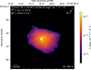 |
Fig. A.1. 1991 pre-COSTAR HST/FOC observation of LK-Hα-233 resampled according to the Nyquist–Shannon sampling theorem, i.e., 2 × 2 pixels2 (0.0287 × 0.0287 arcseconds2) and presented in Fig. 1 in a more compressed version. |
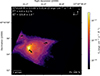 |
Fig. A.3. 1994’s post-COSTAR HST/FOC observation of LK-Hα-233 resampled according to the Nyquist–Shannon sampling theorem, i.e., 2 × 2 pixels2 (0.0287 × 0.0287 arcseconds2) and presented in Fig. 2 in a more compressed version. |
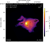 |
Fig. A.5. 1995’s post-COSTAR HST/FOC observation of LK-Hα-233 resampled according to the Nyquist–Shannon sampling theorem, i.e., 2 × 2 pixels2 (0.0287 × 0.0287 arcseconds2) and presented in Fig. 3 in a more compressed version. |
All Tables
All Figures
|
Fig. 1. Left: 1991 pre-COSTAR HST/FOC observation of LK-Hα-233 resampled according to the Nyquist–Shannon sampling theorem (i.e., 2 × 2 pixels2 or 0.0287 × 0.0287 arcseconds2), to ensure individual pixels yield meaningfully polarization measurements. The total flux is color-coded and expressed in units of erg cm−2 s−1 Å−1. Polarization vectors are displayed for [S/N]P ≥ 3, although at this spatial resolution they are difficult to resolve visually (larger images are presented in the appendices). Total flux contours are displayed for 0.8%, 2%, 5%, 10%, 20%, and 50% of the maximum flux. In the top-left corner, we indicate the total flux F, polarization degree P, and polarization angle θ values, integrated over the whole field of view (7 × 7 arcseconds2 in this image). Following the IAU convention, north is up and the polarization angle positively rotates toward the east. Right: Same image but with a spatial binning of 0.1 arcsecond per pixel. The polarization pattern highlighted by the vectors becomes more apparent at this scale. |
| In the text | |
|
Fig. 2. Same as Fig. 1 but for the 1994 post-COSTAR HST/FOC observation of LK-Hα-233. The top panel shows the high-resolution map, with inserts indicating where [S/N]P ≥ 3 polarization vectors are detected. The white dot corresponds to a reseau mark that was masked during the reduction process. The bottom panel shows the medium-resolution map. Due to slightly incorrect pointing, the source appears in the bottom-left corner of the FOC field of view and is partially cut off. The improved image sharpness resulting from the COSTAR corrective optics package is clearly visible. |
| In the text | |
|
Fig. 3. Same as Fig. 2 but for the 1995 post-COSTAR HST/FOC observation of LK-Hα-233. Due to a minor pointing offset, the western extremity of the source falls partially outside the field of view. |
| In the text | |
|
Fig. 4. Medium-resolution polarized flux map from the 1995 post-COSTAR HST/FOC observation of LK-Hα-233. The red cross marks the estimated location of the hidden star. |
| In the text | |
|
Fig. 5. Variation of the total flux (top), polarization degree (middle), and polarization angle (bottom) as a function of increasing aperture radius, centered on the location of the hidden star. Error bars are shown, but may be too small to be visible. |
| In the text | |
|
Fig. 6. The five distinct regions of LK-Hα-233 detected for detailed analysis. The map is the 1995 observation (identical to Fig. 3). Each white circle corresponds to an aperture with a radius of 1 arcsecond. |
| In the text | |
|
Fig. 7. Variability of LK-Hα-233 in total flux (top left), polarized flux (bottom left), polarization degree (top right), and polarization angle (bottom right) as a function of time (in modified Julian date). We accounted for the three HST/FOC observations; however, due to a pointing error which cut off part of the object in 1994, some data points are unavailable from that epoch. Except for the black crosses (full field of view, 7 × 7 arcseconds), all other points correspond to 1 arcsecond aperture radius integration windows at the five different regions presented in Fig. 6. Error bars are shown but may be too small to be visible. |
| In the text | |
|
Fig. A.1. 1991 pre-COSTAR HST/FOC observation of LK-Hα-233 resampled according to the Nyquist–Shannon sampling theorem, i.e., 2 × 2 pixels2 (0.0287 × 0.0287 arcseconds2) and presented in Fig. 1 in a more compressed version. |
| In the text | |
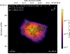 |
Fig. A.2. Same as Fig. A.1 but with a spatial binning of 0.1 arcsecond per pixel. |
| In the text | |
|
Fig. A.3. 1994’s post-COSTAR HST/FOC observation of LK-Hα-233 resampled according to the Nyquist–Shannon sampling theorem, i.e., 2 × 2 pixels2 (0.0287 × 0.0287 arcseconds2) and presented in Fig. 2 in a more compressed version. |
| In the text | |
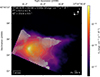 |
Fig. A.4. Same as Fig. A.3 but with a spatial binning of 0.1 arcsecond per pixel. |
| In the text | |
|
Fig. A.5. 1995’s post-COSTAR HST/FOC observation of LK-Hα-233 resampled according to the Nyquist–Shannon sampling theorem, i.e., 2 × 2 pixels2 (0.0287 × 0.0287 arcseconds2) and presented in Fig. 3 in a more compressed version. |
| In the text | |
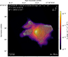 |
Fig. A.6. Same as Fig. A.5 but with a spatial binning of 0.1 arcsecond per pixel. |
| In the text | |
Current usage metrics show cumulative count of Article Views (full-text article views including HTML views, PDF and ePub downloads, according to the available data) and Abstracts Views on Vision4Press platform.
Data correspond to usage on the plateform after 2015. The current usage metrics is available 48-96 hours after online publication and is updated daily on week days.
Initial download of the metrics may take a while.