| Issue |
A&A
Volume 699, July 2025
|
|
|---|---|---|
| Article Number | A37 | |
| Number of page(s) | 15 | |
| Section | Interstellar and circumstellar matter | |
| DOI | https://doi.org/10.1051/0004-6361/202554689 | |
| Published online | 01 July 2025 | |
Spatially resolved centrifugal magnetosphere caught in motion around the secondary component of ρ Oph A
European Organisation for Astronomical Research in the Southern Hemisphere (ESO), Casilla
19001,
Santiago 19,
Chile
★ Corresponding author: This email address is being protected from spambots. You need JavaScript enabled to view it.
Received:
21
March
2025
Accepted:
7
May
2025
Abstract
Aims. The recently discovered spectroscopic binary ρ Oph A is a rare magnetic hot binary system composed of two early B-type stars, comprising a nonmagnetic primary (Aa) and a slightly less massive magnetic secondary (Ab). Using near-IR interferometry, we aim to resolve the system’s astrometric orbit. The high-spectral-resolution VLTI/GRAVITY data also enable further information to be obtained about the two stellar components, and about the centrifugal magnetosphere orbiting the magnetic star.
Methods. We obtained a time-series of K-band interferometric data from VLTI/GRAVITY and analyzed them with the geometrical model-fitting tool PMOIRED. The continuum was used to derive the relative astrometry and relative fluxes of the two components, leading to the astrometric orbital solution. Spectro-interferometry covering the Brγ line was then used to obtain high-angular-resolution information about the dominant magnetospheric cloud in corotation with the magnetic Ab component.
Results. The combination of the astrometric orbital solution and the published radial velocities for both components enabled us to obtain a three-dimensional orbital solution, dynamical masses, and a dynamical parallax. These results are in a good agreement with previous estimates and confirm the previously inferred alignment of the orbital axis and the rotation axis of the Ab component at a much higher precision. A detailed analysis of the Brγ spectro-interferometry then revealed the changing position of the magnetospheric cloud relative to the Ab component. Comparison to the location of the cloud predicted from ρ Oph Ab ’s oblique rotator model and from the Hα emission properties resulted in excellent agreement. We are additionally able to demonstrate that the magnetic star exhibits prograde rotation. This is the first time that the motion of a centrifugal magnetosphere has been detected in angularly resolved observations.
Key words: techniques: interferometric / circumstellar matter / stars: magnetic field / stars: massive / stars: individual: HD 147933
© The Authors 2025
 Open Access article, published by EDP Sciences, under the terms of the Creative Commons Attribution License (https://creativecommons.org/licenses/by/4.0), which permits unrestricted use, distribution, and reproduction in any medium, provided the original work is properly cited.
This article is published in open access under the Subscribe to Open model. This email address is being protected from spambots. You need JavaScript enabled to view it. to support open access publication.
1 Introduction
Magnetic OBA stars comprise approximately 10% of the population of the upper main sequence (Grunhut et al. 2017; Sikora et al. 2019a). Their surface magnetic fields are, with rare exceptions, geometrically simple (approximately dipolar; e.g., Shultz et al. 2018b; Kochukhov et al. 2019) and strong (with surface dipole strengths on the order of several kilogauss; e.g., Sikora et al. 2019b; Shultz et al. 2019b). They are also, without exception, stable: while there is clear and abundant evidence that the surface magnetic field strength, and perhaps also the total magnetic flux, decline over evolutionary timescales (Landstreet et al. 2007; Landstreet et al. 2008; Fossati et al. 2016; Shultz et al. 2019b), over human timescales their magnetic fields show no evidence of reorganization (Shultz et al. 2018b).
Since energy is transported by radiation rather than convection in the outer envelopes of OBA stars, contemporaneous dynamos are not expected. While magnetohydrodynamic (MHD) simulations predict that rotational-convective dynamos should produce extremely strong fields (hundreds of kilogauss) in the convective cores of these stars (Augustson et al. 2016), these should not be able to rise to the stellar surface on evolutionary timescales (Hidalgo et al. 2024). It is therefore unlikely that dynamos sustained by core convection generate measurable hot star magnetic fields, and indeed the magnetic fields of hot stars show no correlation with surface rotation (Sikora et al. 2019b; Shultz et al. 2019b), as would be expected for dynamo fields, and as is observed for cool stars (e.g., Folsom et al. 2016). All of these factors led to the characterization of hot star magnetic fields as “fossil” fields, i.e., remnants of some previous event in the star’s life cycle. While radiative envelopes cannot generate magnetic fields, MHD simulations indicate that once established, they can be preserved almost indefinitely (e.g., Braithwaite & Spruit 2004; Duez et al. 2010).
An important consequence of the stability of fossil magnetic fields is that the spectropolarimetric, spectroscopic, and photometric variability of magnetic early-type stars is dominated by rotation. Thus, in contrast to other hot stars, rotational periods are easily determined, frequently to a precision of around 10−6 d. The most common geometric configuration is a dipole tilted with respect to the rotational axis. This tilt of the magnetic dipole leads to spectropolarimetric variability due to the changing projection of the surface magnetic field as the star rotates. In stars with detectable magnetospheres, this also leads to spectroscopic and photometric variability modulated on the rotational cycle, since the magnetosphere corotates with the star.
One possible avenue for generating fossil fields is via dynamos powered by binary mergers. This scenario has been demonstrated in MHD simulations (Schneider et al. 2019) and accounts for various aspects of the hot star population: binarity is extremely common on the upper main sequence; binarity is extremely rare among magnetic stars (Alecian et al. 2015); and the expected merger fraction is similar to the fraction of hot stars with fossil fields (Sana et al. 2012; de Mink et al. 2013, 2014).
One phenomenon the merger scenario has some difficulty accounting for are the rare magnetic binary systems (e.g., Landstreet et al. 2017; Kochukhov et al. 2018; Shultz et al. 2018a, 2019a), since these would require initially triple or quadruple architectures. While mergers in such systems are by no means unexpected (Marchant & Bodensteiner 2024), obtaining a tightly bound binary as the product of, for example, the merger of a hardened inner binary within a hierarchical triple is hard to explain (Bruenech et al. 2025). Magnetic binaries are therefore objects of particular interest in the study of hot star magnetism, as in addition to the usual advantages of binary stars (e.g., the precise measurement of fundamental parameters), they may ultimately offer some insight into the origin of fossil magnetic fields and the evolutionary pathways open to the stellar population’s brightest members.
Shultz et al. (2025) recently discovered that the nearby magnetic B2 star ρ Oph A (HD 147933) is a previously undetected spectroscopic binary, with two rapidly rotating B-type stars bound in a slightly eccentric 88-day orbit. The system consists of a nonmagnetic primary, ρ Oph Aa, and a slightly less massive magnetic secondary, ρ Oph Ab. The system’s architecture is strikingly similar to that of W601, a somewhat younger, slightly longer-period binary also consisting of two rapidly rotating B-type stars with a magnetic secondary orbiting a nonmagnetic primary (Shultz et al. 2021).
The rotational variability of spectropolarimetric, spectroscopic, and photometric time series data all converge on a rotational period of around 0.74 d (Leto et al. 2020), making ρ Oph Ab one of the most rapidly rotating magnetic B-type stars known. The precisely measured rotational period enables the inclination angle of the rotational axis to be determined, and it is apparently aligned with the orbital axis (as constrained via a comparison of the mass function with masses from evolutionary models).
Due to its strong magnetic field and extreme rotation, ρ Oph Ab is surrounded by a “centrifugal magnetosphere,” that is, a region in which the stellar wind is magnetically confined and forced into corotation with the star by the Lorentz force, with the resulting rotational support preventing gravitational infall of the confined plasma (Townsend & Owocki 2005; Petit et al. 2013). Centrifugal magnetosphere plasma builds up to very high densities before being expelled from the star in centrifugal breakout magnetic reconnection events (ud-Doula et al. 2008; Owocki et al. 2020). This results in several diagnostics that probe different parts of the magnetosphere. Electrons accelerated to semi-relativistic energies by centrifugal breakout lead to gyro-synchrotron radio emission (Drake et al. 1987; Leto et al. 2021; Shultz et al. 2022; Owocki et al. 2022) and beamed electron-cyclotron maser emission (Trigilio et al. 2000, 2011; Das & Chandra 2021; Das et al. 2022). The cool, pre-breakout plasma is detectable via photometric eclipses (when the magnetosphere passes in front of the star; e.g., Landstreet & Borra 1978; Townsend 2008; Berry et al. 2023) as well as via Hα emission (when the magnetosphere is projected to the side of the star; e.g., Grunhut et al. 2012; Rivinius et al. 2013; Oksala et al. 2015; Sikora et al. 2015, 2016; Shultz et al. 2020, 2021). All of these phenomena are present in the case of ρ Oph Ab. The Hα emission of ρ Oph Ab is notably lopsided, with a single large cloud rather than the two clouds that are more commonly seen in single magnetic stars. The only other stars with such asymmetrical emission profiles are also close binaries (Shultz et al. 2018a, 2020), suggesting that dynamical effects play a role in shaping the magnetospheric plasma distribution.
Since ρ Oph A is both bright (V = 5.05) and very close (about 140 pc from the Sun), the predicted angular separation of several milliarcseconds (mas) puts it well within the angular resolution of the Very Large Telescope Interferometer (VLTI), thereby offering an excellent opportunity to precisely measure its orbital inclination, test the hypothesis that the rotational and orbital axes are aligned, and obtain dynamical measurements of the masses of the two stars.
While the primary aim of studying the VLTI/GRAVITY K-band data presented in this work was to obtain astrometric constraints on the binary orbit, the high-spectral-resolution dataset also offers an opportunity to examine the magnetosphere in the Brγ line, and to search for its spectro-interferometric signatures. To date, the only interferometric detection of magnetically bound plasma has been reported from a single observation of HR 5907 by VLTI/AMBER (Rivinius et al. 2012).
In Sect. 2, the VLTI/GRAVITY data are described. The orbital analysis is provided in Sect. 3 and the spectrointerferometric analysis of Brγ in Sect. 4. The results are discussed in Sect. 5, and the conclusions summarized in Sect. 6. Individual observations are provided in Appendix A.
2 VLTI/GRAVITY observations
We used the VLTI (Eisenhauer et al. 2023) instrument GRAVITY (GRAVITY Collaboration 2017) operating in the near-IR K band to collect a total of seven interferometric observations of the ρ Oph A binary system. VLTI was used with the auxiliary telescope (AT) array in the “Large” configuration (from April to September 2023), reaching maximum baselines of ~130 m, which corresponds to the angular scale λ/2Bmax ~ 1.75 mas in the K band. The four ATs have primary mirror sizes of 1.8 m and are equipped with the dedicated adaptive optics system NAOMI (Woillez et al. 2019). An example observation zoomed in on the Brγ line is shown in Fig. 1, with the different telescope baselines and triangles specified by the corresponding telescope locations on the VLTI platform in the upper left panel. For the layout of the telescope locations, see Fig. 10 in the VLTI manual1.
The GRAVITY instrument was used in the single field onaxis mode, and in high spectral resolution (R= 4000) covering the entire K band (1.98 to 2.40 μm). Every interferometric “snapshot” (~1 hr observing time including overheads) consisted of observation of the science target and the calibrator star HD 145836 (K = 5.1, uniform disk diameter =0.469 ± 0.011 mas, spectral type K0 III). For the reduction and calibration of the data, we used the dedicated European Southern Observatory (ESO) GRAVITY pipeline version 1.6.6 and the EsoReflex software (Freudling et al. 2013). The interferometric observables from GRAVITY covering the K band include spectra (bottom left panel of Fig. 1), calibrated closure phases (T3PHI, one for each telescope triangle per observation; second column of Fig. 1), differential phases (DPHI, one for each telescope pair per observation; third column), and calibrated visibilities (|V|, one for each telescope pair per observation; fourth column). Each of the individual science and calibrator observations consisted of an object–sky–object–object sequence, resulting in three sets of interferometric observables of the science target for each snapshot. Variation in the observables (particularly in |V|) is noticeable in the three observations within each snapshot due to the Earth’s rotation causing changes in the projected baselines. The seven snapshots are of very good quality with the exception of the one taken on reduced Julian date (RJD) 60082, which was marked as poorly executed by the ESO observing staff. While the RJD 60082 observation is of noticeably poor quality compared to the other snapshots (see Fig. A.3), it could still be used in our analysis with certain limitations. The reduced and calibrated data will be made available in the Optical Interferometry Database2 (Haubois et al. 2014).
For the modeling and visualization of the GRAVITY data we used the Python code Parametric Modeling of Optical InteRferomEtric Data3 (PMOIRED; Mérand 2022). PMOIRED enables geometrical model fitting to GRAVITY data by least-squares minimization to obtain the best-fit parameters and includes various capabilities such as grid-searching for the relative positions of components in multiple stellar systems, and fitting of spectrointerferometric signatures with spectral line profiles if the data have sufficient spectral resolution. Other features include a bootstrapping algorithm for the determination of realistic parameter uncertainties and a correction of the GRAVITY spectra for telluric features. The telluric correction enables an assessment of the accuracy of the wavelength calibration, which is known to be at least ~0.02% (Gallenne et al. 2023). The telluric fitting of the ρ Oph A data suggests an accuracy of ~0.03% (~9 km s−1) or better, but we conservatively assumed an error of 0.05% (~ 15 km s−1) for the radial velocities (RVs) derived from GRAVITY data by adding this error quadratically to the bootstrapped error from the model fit.
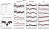 |
Fig. 1 PMOIRED geometrical model fit to the Brγ region of GRAVITY data taken on RJD 60139. The upper left panel shows the (u, v) coverage, the lower left panel the normalized Brγ line profile (NFLUX), and the remaining panels the interferometric observables’ closure phase (T3PHI), differential phase (DPHI), and the absolute visibility (|V|). The data (black with gray error bars) are overplotted along with the model fit (red). The blue dots in the NFLUX and DPHI panels represent the continuum region used for normalization. The baselines and telescope triangles are given in the corner of each panel, and their colors correspond to the (u, v) coverage panel. |
3 Orbital analysis
To determine the relative astrometric positions from the seven GRAVITY snapshots, we used PMOIRED to fit the T3PHI and |V| observables with a simple geometrical model consisting of two uniform disks (UDs) with fixed diameters of 0.3 and 0.2 mas, representing the ρ Oph Aa and Ab components, respectively. The UD diameters of the two stars were estimated from the absolute radii and the distance determined by Shultz et al. (2025), and are equivalent to unresolved point sources at the angular resolution of the data. The free parameters in the astrometric fitting are the astrometric offset ρ of Ab relative to Aa, the astrometric position angle (PA; measured from north to east), and the K band flux ratio between the components f = fAb/fAa.
For the binary fitting, we selected the K-band wavelength interval between 2.10 and 2.35 μm, and we re-binned the data from the original spectral resolution R ~ 4000 to R ~ 100. Using the grid search algorithm implemented in PMOIRED, the fit to all of the seven datasets successfully converged, resulting in ρ ranging from ~2.3 to ~8.4 mas, with reduced χ2 between 0.5 and 5.2 for the high quality epochs, and 9.4 for the low quality dataset from RJD 60082. An example of the re-binned data and the corresponding binary model fit is shown in Fig. A.1, and the resulting parameters, with the final values and uncertainties determined by bootstrapping, are given in Table A.1.
To obtain a three-dimensional orbital solution, we combined the relative astrometry determined above with the RVs measured by Shultz et al. (2025). We used two different software packages for the orbital solution: the IDL code orbfit-lib4 based on the Newton-Raphson method (Schaefer et al. 2016), and the Python code spinOS5 with the implemented Markov chain Monte Carlo (MCMC) method (Fabry et al. 2021a,b). The weights of the two datasets were adjusted so that they contribute approximately equally to the total residuals. The two resulting sets of orbital parameters, as well as the dynamical masses and the distance to the system, are fully consistent with each other (Table 1). The spinOS MCMC method gives considerably smaller parameter uncertainties, except for the angular semimajor axis (a″), which for the spinOS solution has to be computed from the fitted total mass and distance. The results agree well with the spectroscopic orbital parameters given by Shultz et al. (2025), which are provided for comparison in the final column of Table 1. The resulting astrometric orbit and RV curves computed from the orbfit-lib solution are plotted in Figs. 2 and 3, respectively.
Orbital solutions.
4 Spectro-interferometric analysis
The relatively high spectral resolution of the GRAVITY data (R= 4000) enables analysis of normalized spectral line profiles (NFLUX) in the K band and their corresponding spectrointerferometric signatures in the T3PHI, DPHI, and |V| observables. In our data, spectro-interferometric signal is detected in two spectral lines: the hydrogen line Brγ and He I λ21126. For the geometrical model fitting of the spectro-interferometry described below, we used all of these four observables except for the low-quality epoch RJD 60082, for which we were forced to discard the T3PHI and |V| data (see below).
4.1 Brγ
The hydrogen line Brγ is the most prominent line in the K band spectra of ρ Oph A. Analogous to Hα in the visible, Brγ shows a blended, broad absorption profile from the two rapidly rotating binary components, and in all but one dataset also an emission bump from the magnetosphere. Figure 4 compares Brγ to Hα at similar rotational phases, demonstrating that emission is seen in Brγ at the expected velocities. The emission bumps in these datasets are highly shifted in RV and located outside of the broad absorption profile, indicating that ρ Oph Ab was caught at rotational phases when the magnetosphere was projected next to the star. The seventh dataset taken on RJD 60171 (phase 0.738 in Fig. 4) shows no emission bump; this is expected, as Hα does not display emission at this phase, which occurs when the magnetospheric cloud is eclipsed behind the star (see Shultz et al. 2025).
Based on the rigidly rotating magnetosphere (RRM) model (Townsend & Owocki 2005), the inner edge of the magnetospheric cloud should be located above the Kepler rotation radius ![Mathematical equation: $\[R_{\mathrm{K}}=1.93_{-0.03}^{+0.08} ~R_{*}\]$](/articles/aa/full_html/2025/07/aa54689-25/aa54689-25-eq1.png) (Shultz et al. 2025), a prediction consistent with the properties of the star’s Hα emission. Given the velocity range of Hα at maximum emission, the outermost extent of the cloud is around 4.4 R⊙ (see below). At a distance of about 140 pc, the expected maximum projected angular extent of the magnetosphere – occurring at rotational phases 0.0 and 0.5 – should then be ~0.25 mas, and it should be separated from the center of the star at the same phases by ~0.2 to ~0.45 mas. Given the high quality and angular resolution of the GRAVITY data, such an offset should introduce a small but detectable signal in the Brγ DPHI (~1° at the longest baselines), similar to what was detected by Rivinius et al. (2012) for HR 5907 in AMBER data. The detectability of the magnetospheric cloud is further aided by the fact that it surrounds the secondary component in a low contrast binary, which amplifies the expected DPHI signal, and introduces small but detectable signals in the T3PHI and |V| observables as well.
(Shultz et al. 2025), a prediction consistent with the properties of the star’s Hα emission. Given the velocity range of Hα at maximum emission, the outermost extent of the cloud is around 4.4 R⊙ (see below). At a distance of about 140 pc, the expected maximum projected angular extent of the magnetosphere – occurring at rotational phases 0.0 and 0.5 – should then be ~0.25 mas, and it should be separated from the center of the star at the same phases by ~0.2 to ~0.45 mas. Given the high quality and angular resolution of the GRAVITY data, such an offset should introduce a small but detectable signal in the Brγ DPHI (~1° at the longest baselines), similar to what was detected by Rivinius et al. (2012) for HR 5907 in AMBER data. The detectability of the magnetospheric cloud is further aided by the fact that it surrounds the secondary component in a low contrast binary, which amplifies the expected DPHI signal, and introduces small but detectable signals in the T3PHI and |V| observables as well.
Visual inspection of the interferometric observables in the datasets with the magnetospheric emission bump reveals rather complex features (especially in DPHI), and there is indeed a clear signal at a wavelength identical to the emission bump in the spectrum (see Fig. 1). In addition, there is a broader signal corresponding to the relative astrometric offset of the two stellar components, whose absorption profiles should also be RV-shifted following the orbital solution.
For the detailed analysis of the Brγ line profile and spectrointerferometry, we selected a 24 nm-wide region centered on the Brγ vacuum wavelength λBrγ,vac = 2.1661178 μm, and we employed PMOIRED to fit a geometrical model to the unbinned data (R ~ 4000). We used the same representation for the two stellar components as in the binary fitting procedure, and we kept the relative astrometry (ρ and PA) and the flux ratio (f) fixed at the previously determined values (Sect. 3 and Table A.1). Then, we added the following model components: two Gaussian absorption line profiles representing the lines of the two stellar components, and a Gaussian emission line profile representing the emission bump from the magnetosphere. Each of these components is defined by the line full width at half maximum (FWHM) and peak amplitude, the RV shift of the line center, and the astrometric position (again fixed at the previously determined values for the two stars). The astrometric position of the magnetosphere was allowed to converge from a starting position corresponding to the magnetic Ab component. While the RVs of the stellar components could have been fixed at the values derived from the orbital solution (Sect. 3), the GRAVITY data proved good enough to fit them, enabling an additional check of the validity of our orbital solution.
The geometrical model described above proved to be a good representation of the Brγ region for the five good quality datasets featuring the magnetospheric emission bump, namely the epochs RJD 60054, 60112, 60139, 60172, and 60205, with all of the free parameters (11 in total) successfully converging. An example of the fit is shown in Fig. 1 (for the remaining epochs see Figs. A.2 to A.7), with the components of the corresponding model spectrum shown in Fig. 5.
Regarding the lower quality dataset from RJD 60082, we were forced to discard the T3PHI and |V| observables due to the lack of any discernible spectro-interferometric signal in the noisy data. The DPHI part, on the other hand, shows a clear signal from the magnetosphere for three out of the six baselines, while for the other three the data are again too noisy. The DPHI and the line profile were successfully fitted after fixing the FWHM and peak amplitudes of the three line components at the averaged best-fit values determined from the other five epochs, with only the magnetosphere position and the three RVs left as free parameters.
As for the RJD 60171 epoch, no discernible signal from the magnetosphere can be seen in Brγ, and we were able to fit only the two line components corresponding to the two stars. This is consistent with the expectation that at this rotational phase the magnetosphere is eclipsed by its host star.
As with the binary positions determined in Sect. 3, the final values of all the converged parameters and their uncertainties were obtained by the bootstrapping algorithm implemented in PMOIRED. The resulting RVs of the two stars and RVs and astrometric positions of the magnetospheric cloud are listed in Table A.2.
The main goal of this analysis was to provide the astrometric positions and RVs of the magnetosphere, as well as RVs of the two stars for all seven epochs. With the exception of RJD 60171, the astrometric positions of the magnetosphere converged to a relative offset of a few tenths of mas from the Ab component, while the magnetosphere RVs were found to vary around +600 km s−1 or −600 km s−1, matching the expectations (see below for a detailed comparison). Due to the lack of magnetospheric signal at RJD 60171, the magnetosphere position and RV could not be fitted, but we can safely assume that the magnetosphere position in this case coincides with the Ab component, while its RV is close to the systemic velocity; in this case we adopted an error bar of ±230 km s−1, corresponding to the stellar v sin i. The stellar RVs are shown in Fig. 3 as empty symbols, and demonstrate a reasonable agreement with both the RVs measured by Shultz et al. and our orbital solution despite the broadness of the line profiles and the relatively low spectral resolution of GRAVITY (compared to high-resolution spectrographs).
Figure 6 compares the RVs measured for the Brγ emission bump to the velocities of peak emission measured from Hα using ESPaDOnS data. The top panel of Fig. 6 shows the H α emission equivalent widths (EWs) measured by Shultz et al., folded with the star’s rotational period. These were obtained by measuring the EW between about ±1000 km s−1 (the approximate span of the emission profile) of the observed Hα line, and subtracting the EW of a synthetic binary spectrum (see Fig. 4). The emission EWs vary with a double-wave pattern, illustrated with a harmonic fit, with two local maxima corresponding to phases at which the magnetosphere is seen face-on, and local minima corresponding to phases at which the magnetosphere is either eclipsing or eclipsed by the star. As demonstrated by Shultz et al., these phases respectively correspond to the maxima and the nulls of the longitudinal magnetic field curve, i.e., phases at which the magnetic axis is closest to alignment with the line of sight, and Article number, page 6 of 15 phases at which the magnetic equator bisects the visible stellar disk.
The bottom panel of Fig. 6 shows the RVs of the Hα and Brγ emission peaks, also folded with the rotational period. A harmonic fit to the Hα data follows the expected sinusoidal pattern, with the velocity of peak emission varying smoothly between ±600 km s−1. Emission EW minima (i.e., phases at which the cloud is either eclipsing or eclipsed) were not used in the fit, as the emission peak velocities at these phases are unreliable. The velocities obtained from Brγ spectro-interferometry follow the expected variation from Hα very closely.
The positions of the magnetosphere relative to the Ab star are compared to the predictions of the rotational, magnetic, and magnetospheric model parameters determined by Shultz et al. (2025) in Fig. 7. The top panels of Fig. 7 show a schematic model of the projected location of the dominant magnetospheric cloud at various rotational phases. The inner edge of the cloud is placed at the Kepler corotation radius RK = 1.9 R* (dashed line in the upper left panel). The radius of maximum emission rmax, shown by the solid line, was inferred from the RV of the Hα emission line peak, vmax = −600 km s−1: since the cloud is in strict corotation with the star, RV maps linearly to projected distance from the center of the star such that rmax = vmax/v sin i = 2.6 R*. The outermost extent of the cloud rout ~ 4.4 R* (dotted line) was similarly inferred from the RV at which the emission line disappears. The star’s rotation axis is inclined at an angle irot = 71° from the line of sight, which is taken from the orbital fit (Sect. 3) and matches the rotational inclination determined by Shultz et al. (73 ± 5°). The magnetic field, assumed to be a dipole, is then tilted from the rotational axis at an angle β = 62°. The angle β was determined as one of the oblique rotator model parameters inferred from magnetic modeling of the longitudinal magnetic field curve; the oblique rotator model parameters were verified via direct comparison to the circular polarization profiles (Shultz et al. 2025). As can be seen from the model, the cloud begins at phase 0.0 to the left of the star, at maximum negative RV and maximum projected area (corresponding to maximum emission; see Fig. 6). Since the cloud is in the magnetic equatorial plane, this phase also corresponds to a nearly pole-on view of the magnetic field. Between phases 0.2 and 0.3 the cloud eclipses the star, corresponding to the magnetic equator crossing the line of sight. The cloud then moves to the right of the star and positive RV, as the negative magnetic pole moves into the line of sight; passes behind the star at phase 0.7, corresponding to the second magnetic null; and then reappears with negative RV to the left of the star.
The bottom two rows of Fig. 7 show the model at the rotational phases of the GRAVITY observations, comparing the expected position and RV of the cloud to the positions and velocities determined from spectro-interferometric modeling described above. Here the rotational axis has been rotated in the plane of the sky to be perpendicular to the longitude of the ascending node Ω = 303°, as should be the case if the spin and orbital axes are aligned. In general there is good agreement between observations and models. For the observations on RJDs 60205, 60054, and 60172, astrometric and model positions overlap within the 1σ error ellipses. The error ellipse of the observation on RJD 60112 is just in contact with the expected outer extent of the cloud. The error ellipse of the observation of RJD 60139 is well outside of the expected cloud position; however, the cloud size assumed in the astrometric modeling (dashed circle) indicates an overlap with the cloud position, and the measured PA matches the PA of the cloud.
Two observations deserve closer examination. First is the observation on RJD 60171, for which no cloud position could be determined, and no Brγ emission could be detected. The astrometric position of the cloud shown in Fig. 7, at the exact center of the star, is purely nominal, and there is no error ellipse. As can be seen from the model, this observation was acquired at a rotational phase at which the cloud is behind the star. The inability to detect the cloud is therefore perfectly consistent with the model.
The other observation of note is the one acquired on RJD 60082. In this case, the RV matches expectations, and the cloud’s y-position matches the model, but its x-position is offset to the wrong side of the star. While the error ellipse is close to the expected position of the cloud, it is not quite in 1σ agreement. This observation has the worst quality of the dataset, with only three useful baselines and only the DPHI interferometric observable. It is therefore unsurprising that it does not agree as well with the model as the other five data points in which the cloud’s position could be detected. Notably, the higher-quality observation on 60112 was obtained at a similar rotation phase, and is in much better agreement with the expected cloud position.
To examine the influence of different modeling assumptions on the astrometric position of the cloud, the bottom right panel of Fig. 7 shows the variations in the cloud’s central positions and the sizes and PAs of the error ellipses for four different cloud models: UDs with radii of 0.2, 0.3, and 0.4 mas, and a Gaussian with a FWHM of 0.2 mas. These changes have essentially no impact.
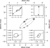 |
Fig. 2 Astrometric orbit (dashed line) with the primary nonmagnetic Aa component at the center (star symbol), the line of nodes (gray line), the ascending node (empty gray circle), and the periastron position (plus sign). The calculated positions on the orbit for the observation epochs (x symbols) coincide with the astrometric measurements (error ellipses corresponding to 5σ uncertainties), which are too small to be seen in the main plot. The inset plots show the zoomed-in areas around the measurements. |
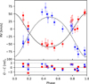 |
Fig. 3 Top: computed RV curves of the Aa and Ab components (solid and dashed curves, respectively) overplotted with RVs for the Aa and Ab components measured by Shultz et al. (filled red squares and blue circles, respectively) and RVs measured from the Brγ signature in GRAVITY data (empty red squares and blue circles, respectively; see Sect. 4). The latter RVs were not used for the orbital solution and are shown only for comparison. Bottom: residuals in units of σ. |
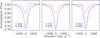 |
Fig. 4 Comparison of Brγ (red) and Hα (blue) at similar rotation phases (labels in lower-left corners). The dashed blue line is a synthetic spectrum that helps highlight the location of the Hα emission. Note that emission is neither expected nor seen near phase 0.7 (middle). |
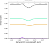 |
Fig. 5 Model spectra obtained for the epoch of RJD 60139. The green spectrum is the Aa component with its continuum flux fixed to 1.0, the orange spectrum is the Ab component with f = fAb/fAa = 0.71, the purple spectrum is the magnetospheric emission with no continuum contribution, and the black spectrum is the sum of the three components. |
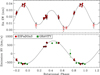 |
Fig. 6 Top: Hα emission EW folded with the rotational period, demonstrating the double-wave character of the variation. The approximate continuum level corresponds to the null line. Points with no emission (from which useful RVs cannot be measured) are indicated by open circles. Bottom: RVs measured from the emission peaks of Hα and the RVs obtained from the Brγ line fitting, both folded with the rotational period. In both panels the black curve shows a harmonic fit to the ESPaDOnS data. |
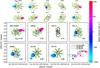 |
Fig. 7 Top: model showing the projected position of the main magnetospheric cloud in rotational phase increments of 0.1. Cloud color indicates RV, as indicated by the color bar. The rotational axis is shown with the orange line. In the top left, dashed, solid, and dotted lines respectively indicate the Kepler corotation radius, the radius of maximum emission, and the outer extent of emission. Bottom: comparison of the expected location of the main magnetospheric cloud and the position recovered from the GRAVITY spectro-interferometry in Brγ. Astrometric locations are indicated by the star symbol, uncertainties in the position by error ellipses, and the assumed angular size of the cloud used in the fitting by the dashed circle. Bottom right: comparison of cloud positions and error ellipses inferred from different models: a Gaussian model with a 0.2 mas FWHM and UD models with radii of 0.2, 0.3, and 0.4 mas. Individual observations are color-coded. The adoption of different modeling assumptions has no significant influence on disk position or error ellipse properties. |
4.2 He I 21126
The He I λ21126 line shows an absorption line profile, and a weak signal in DPHI at the two epochs corresponding to the largest angular separation between the binary components (RJDs 60053 and 60139). The DPHI signature can be reproduced by introducing a Gaussian line profile for each component. The line profile is defined in the PMOIRED geometrical model in the same way as described above for Brγ, but with the central wavelength of 2.112583 μm.
The results from the two epochs indicate that the Ab component has a slightly stronger absorption, which is consistent with it being a He-strong magnetic chemically peculiar star. The RVs of the two components remain similar to those determined from Brγ, albeit with much larger uncertainties, and therefore are not useful for further constraining the binary orbit.
5 Discussion
5.1 Comparison with previous results
Shultz et al. (2025) determined the orbital elements of ρ Oph A solely from RV measurements. As can be seen from Table 1, the results found here are in agreement in all particulars within the (generally much larger) uncertainties accompanying the original solution. The value of T0 given in the third column of Table 1 is almost exactly 75 orbital cycles removed from the more precise period determined by astrometric modeling, and is therefore functionally equivalent.
Shultz et al. additionally derived a distance of 139 ± 3 pc, using the Gaia Data Release 3 parallaxes for the nearby stars in the ρ Oph cluster, as they judged the parallax for ρ Oph A itself to be unreliable due to its high renormalized unit weight error (RUWE) of 3.4 (where RUWE > 1 is considered to be indicative of a poor fit due to binarity). The distances determined astrometrically from the orbital fit are in almost perfect agreement with this value.
5.2 Spin–orbit alignment
Shultz et al. noted that their orbital inclination iorb = 69 ± 11° was consistent with the rotational inclination irot = 73 ± 5°. These values were independently determined: iorb was found from comparison of the mass function to evolutionary models and the locations of the two components on the Kiel diagram, whereas irot was found from the stellar radius, the rotational period, and the velocity broadening of absorption lines.
The astrometric value of iorb determined here, 71.31 ± 0.07° (orbfit-lib solution), is much more precise than the previous value, and is functionally identical to irot, suggesting that the orbital and rotational axes of ρ Oph Ab are indeed in perfect alignment. Consistent with this, the astrometric comparison of the expected versus measured position of the magnetospheric cloud shown in Fig. 7 provides a very good match if the rotational axis is tilted in the plane of the sky to match Ω, as would be expected for spin–orbit alignment.
In addition to alignment of the orbital and rotational axes, comparison of the astrometric positions to the RVs of the clouds reveals that ρ Oph Ab also exhibits prograde rotation: both the orbit and rotation are counterclockwise, with maximum and minimum RVs occurring at the southeast and northwest, respectively.
ρ Oph Ab therefore joins the still very limited sample of stars for which the inclination of the rotation axis from the line of sight, the tilt of the rotational axis in the sky, and the direction of rotation have been determined. Similar constraints have sometimes been possible using the starspot tracking method in eclipsing binaries, finding a variety of systems exhibiting aligned, misaligned, prograde, and retrograde rotation (e.g., Balaji et al. 2015; Albrecht et al. 2022; Li et al. 2024). Interferometric methods have placed similar constraints on the nearby classical Be star and a wide eccentric binary Achernar (which exhibits prograde rotation but a misaligned rotation axis; Domiciano de Souza et al. 2014; Kervella et al. 2022), as well as for the Be + stripped star binaries HD 6819 and HR 2142, which both exhibit aligned and prograde rotation, as would be expected given that these are post-mass-transfer binaries (Klement et al. 2025, 2024).
5.3 Formation of the system and origin of the fossil magnetic field
The almost perfect alignment of the orbital and rotational angular momentum vectors is easily explained in a formation scenario in which both stars were born from the same molecular cloud, and therefore inherited the cloud’s angular momentum vector. However, it may challenge the hypothesis that fossil magnetic fields are generated by binary mergers (e.g., Schneider et al. 2019).
A merger scenario would need to begin with a hierarchical triple, consisting of the nonmagnetic 10 M⊙ primary and two ~4 M⊙ stars, with the smaller stars in a very close orbit. For the smaller stars to merge, their orbit would need to decay, which could happen by one of three mechanisms: (1) stellar evolution, in which one of the stars overflows its Roche lobe; (2) tidal friction; or (3) dynamical interactions. Given the system’s age, (1) is ruled out a priori. Tidal friction between B-type stars is inefficient over such timescales, and is unlikely to shrink the orbit sufficiently to produce a merger (Zahn 1977). The remaining option, dynamical interactions, would likely be very chaotic. Assuming that the orbit around the primary is not destroyed by the energy released by the merger, the result should still be a much wider and more eccentric orbit than is observed (Bruenech et al. 2025). Furthermore, the perfect alignment of the merger product’s angular momentum vector with the orbit is also very unlikely in this scenario.
The difficulty in reconciling the orbital and rotational properties of the system with a merger suggests that the fossil magnetic field must have some other origin. Here there are two possibilities. The first is that the magnetic flux is simply inherited from the molecular cloud, frozen and amplified during the collapse of the star. High-resolution simulations suggest that this scenario is plausible, but the results are highly sensitive to numerical resolution (Wurster et al. 2022). In the case of binary systems such as ρ Oph A this scenario raises the question of why only one of the stars is magnetic, and might require turbulent processes in the cloud preferentially gathering magnetic flux into one of the cores. Another difficulty concerns the role of convection during the protostellar phase, which should rapidly destroy magnetic flux inherited from the protostellar cloud, unless the rapid formation of a radiative core, or rapid transition to a fully radiative star, can preserve some of the inherited flux (Schleicher et al. 2023).
The other non-merger possibility is that the fossil field was generated by a rotational-convective dynamo during the protostellar phase. The principle difficulty with this scenario is that the magnetic activity cycles expected in convective cores should have much shorter timescales (~ years, as shown by MHD simulations of the convective cores of A-type stars; Hidalgo et al. 2024) than the timescale over which radiation freezes out convection, meaning that the radiative zone should end up consisting of thin layers with opposite magnetic polarities that cancel one another out (as described in Sect. 4.5 of the review by Braithwaite & Spruit 2017). Jermyn & Cantiello (2021) have suggested just this sort of magnetic layering as a consequence of dynamo action in the opacity-bump convection zones embedded in the radiative envelopes of early-type stars. Putting this difficulty aside, it is interesting to note that the magnetic secondary is more rapidly rotating than the primary. Assuming that the primary’s rotational axis shares the secondary’s perpendicular orientation to the orbital plane, its measured velocity broadening of 206 ± 5 km s−1 implies a rotational period of about 1 day, indeed slower than the magnetic secondary. Given that the primary is not magnetic, it is unlikely to have experienced significant spin-down since arriving on the zero-age main sequence, i.e., its present rotational period is probably comparable to its original period. By contrast, the magnetic secondary should be losing angular momentum rapidly through its corotating magnetosphere (e.g., ud-Doula et al. 2009; Petit et al. 2013). Its calculated spin-down age of 5 Myr matches the estimated age of the ρ Oph group, suggesting that it was indeed rotating close to critical velocity when it arrived on the zero-age main sequence.
If ρ Oph Ab was initially a much more rapid rotator than the primary, and this dichotomy extended back to the system’s earliest history, this might explain the magnetic field. More rapid rotation on the pre-main sequence would imply a more vigorous rotational-convective dynamo, and thus a stronger magnetic field, than possessed by the primary; when the stars’ envelopes became radiative, the weaker magnetic field of the primary was quickly destroyed by flux decay, while the stronger magnetic field of the secondary was able to freeze itself into the radiative zone. One implication of this scenario is that in young magnetic binary systems, we should generally expect the magnetic star to be the more rapid rotator, while in more evolved systems the magnetic star should rotate more slowly than the nonmagnetic companion due to magnetic braking.
6 Conclusions
Orbital elements of the magnetic binary ρ Oph A constrained with VLTI/GRAVITY observations confirm the spectroscopically inferred binarity of the system, as well as the gross properties of the orbit (period, semimajor axis, eccentricity, etc.). The orbital inclination, iorb = 71.31 ± 0.07°, is identical within the uncertainties to the rotational inclination of the magnetic star ρ Oph Ab, irot = 73 ± 5°.
We obtained a highly significant detection of the dominant magnetospheric cloud orbiting ρ Oph Ab from spectrointerferometric data, with the strongest signal appearing in the differential phases. The detection and the astrometric measurement of its changing position around the magnetic secondary furthermore demonstrate that (1) the magnetic star’s rotational axis is tilted in the plane of the sky by the same angle as the longitude of the ascending node, i.e., the rotational axis is perpendicular to the orbital plane, and (2) the magnetic star exhibits prograde rotation.
This is the first time that a hot star magnetosphere has been detected astrometrically, and therefore the first case in which the direction of a magnetic early-type star’s rotation has been determined. Astrometric detection of the magnetosphere additionally provides further confirmation of the gap between the inner edge of the magnetically confined plasma of a circumstellar magnetosphere (with an inner boundary at the Kepler corotation radius) and the surface of the star, as expected from the RRM model.
Data availability
The reduced and calibrated GRAVITY data are available at https://oidb.jmmc.fr/collection.html?id=512015b1-fb46-4cde-a015-b1fb46ccdec6.
Acknowledgements
This work is based on observations collected at the European Southern Observatory under ESO programme 111.24M8.001. MES acknowledges financial support from the ESO SSDF. This research has made use of the Jean-Marie Mariotti Center Aspro service6. This research has made use of the Jean-Marie Mariotti Center OIFits Explorer service7. This research has made use of the Jean-Marie Mariotti Center SearchCal service, which involves the JSDC and JMDC catalogues8.
Appendix A Detailed results from the fitting of GRAVITY data
The relative astrometry and flux ratios for all the GRAVITY epochs are detailed in Table A.1, while the RVs for the stellar components and the RVs and the astrometric positions of the magnetospheric cloud derived from the GRAVITY spectro-interferometry are given in Table A.2. An example of the binary model fit to GRAVITY data is shown in Fig. A.1, while the fits to the Brγ spectrointerferometry are shown in Figs. A.2 to A.7 (except for RJD 60139, which is shown in Fig. 1).
Relative astrometric positions and flux ratios of the ρ Oph A binary determined from GRAVITY data.
RVs of the stellar components and RVs and astrometric positions of the magnetospheric cloud determined from GRAVITY data.
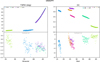 |
Fig. A.1 Top: Binary fit to the re-binned GRAVITY data taken on RJD 60205. The data consist of four sets of closure phases (T3PHI in units of degrees) for each telescope triangle and six sets of visibilities (|V|) for each telescope pair (colored points). The data are overplotted with the binary model fit (dashed lines). Bottom: Residuals in units of σ. The x axes correspond to the spatial frequency in the unit of M λ. The binary fit indicates a relative offset ρ ~ 2.3 mas, PA ~ 223°, and f = fAb/fAa ~ 0.7. The reduced χ2 of the fit is ~2.7. |
References
- Albrecht, S. H., Dawson, R. I., & Winn, J. N. 2022, PASP, 134, 082001 [NASA ADS] [CrossRef] [Google Scholar]
- Alecian, E., Neiner, C., Wade, G. A., et al. 2015, in New Windows on Massive Stars, IAU Symposium, 307, 330 [Google Scholar]
- Augustson, K. C., Brun, A. S., & Toomre, J. 2016, ApJ, 829, 92 [Google Scholar]
- Balaji, B., Croll, B., Levine, A. M., & Rappaport, S. 2015, MNRAS, 448, 429 [Google Scholar]
- Berry, I. D., Shultz, M. E., Owocki, S. P., & ud-Doula, A. 2023, MNRAS, 523, 6371 [Google Scholar]
- Braithwaite, J., & Spruit, H. C. 2004, Nature, 431, 819 [Google Scholar]
- Braithwaite, J., & Spruit, H. C. 2017, Roy. Soc. Open Sci., 4, 160271 [NASA ADS] [CrossRef] [Google Scholar]
- Bruenech, C. W., Boekholt, T., Kummer, F., & Toonen, S. 2025, A&A, 693, A14 [NASA ADS] [CrossRef] [EDP Sciences] [Google Scholar]
- Das, B., & Chandra, P. 2021, ApJ, 921, 9 [NASA ADS] [CrossRef] [Google Scholar]
- Das, B., Chandra, P., Shultz, M. E., et al. 2022, MNRAS, 517, 5756 [Google Scholar]
- de Mink, S. E., Langer, N., Izzard, R. G., Sana, H., & de Koter, A. 2013, ApJ, 764, 166 [Google Scholar]
- de Mink, S. E., Sana, H., Langer, N., Izzard, R. G., & Schneider, F. R. N. 2014, ApJ, 782, 7 [Google Scholar]
- Domiciano de Souza, A., Kervella, P., Moser Faes, D., et al. 2014, A&A, 569, A10 [NASA ADS] [CrossRef] [EDP Sciences] [Google Scholar]
- Drake, S. A., Abbott, D. C., Bastian, T. S., et al. 1987, ApJ, 322, 902 [NASA ADS] [CrossRef] [Google Scholar]
- Duez, V., Braithwaite, J., & Mathis, S. 2010, ApJ, 724, L34 [Google Scholar]
- Eisenhauer, F., Monnier, J. D., & Pfuhl, O. 2023, ARA&A, 61, 237 [NASA ADS] [CrossRef] [Google Scholar]
- Fabry, M., Hawcroft, C., Frost, A. J., et al. 2021a, A&A, 651, A119 [NASA ADS] [CrossRef] [EDP Sciences] [Google Scholar]
- Fabry, M., Hawcroft, C., Mahy, L., et al. 2021b, spinOS: SPectroscopic and INterferometric Orbital Solution finder, Astrophysics Source Code Library [record ascl:2102.001] [Google Scholar]
- Folsom, C. P., Petit, P., Bouvier, J., et al. 2016, MNRAS, 457, 580 [Google Scholar]
- Fossati, L., Schneider, F. R. N., Castro, N., et al. 2016, A&A, 592, A84 [NASA ADS] [CrossRef] [EDP Sciences] [Google Scholar]
- Freudling, W., Romaniello, M., Bramich, D. M., et al. 2013, A&A, 559, A96 [NASA ADS] [CrossRef] [EDP Sciences] [Google Scholar]
- Gallenne, A., Mérand, A., Kervella, P., et al. 2023, A&A, 672, A119 [NASA ADS] [CrossRef] [EDP Sciences] [Google Scholar]
- GRAVITY Collaboration (Abuter, R., et al.) 2017, A&A, 602, A94 [NASA ADS] [CrossRef] [EDP Sciences] [Google Scholar]
- Grunhut, J. H., Rivinius, T., Wade, G. A., et al. 2012, MNRAS, 419, 1610 [CrossRef] [Google Scholar]
- Grunhut, J. H., Wade, G. A., Neiner, C., et al. 2017, MNRAS, 465, 2432 [NASA ADS] [CrossRef] [Google Scholar]
- Haubois, X., Bernaud, P., Mella, G., et al. 2014, SPIE Conf. Ser., 9146, 914600 [Google Scholar]
- Hidalgo, J. P., Käpylä, P. J., Schleicher, D. R. G., Ortiz-Rodríguez, C. A., & Navarrete, F. H. 2024, A&A, 691, A326 [NASA ADS] [CrossRef] [EDP Sciences] [Google Scholar]
- Jermyn, A. S., & Cantiello, M. 2021, ApJ, 923, 104 [NASA ADS] [CrossRef] [Google Scholar]
- Kervella, P., Borgniet, S., Domiciano de Souza, A., et al. 2022, A&A, 667, A111 [NASA ADS] [CrossRef] [EDP Sciences] [Google Scholar]
- Klement, R., Rivinius, T., Gies, D. R., et al. 2024, ApJ, 962, 70 [NASA ADS] [CrossRef] [Google Scholar]
- Klement, R., Rivinius, T., Baade, D., et al. 2025, A&A, 694, A208 [NASA ADS] [CrossRef] [EDP Sciences] [Google Scholar]
- Kochukhov, O., Johnston, C., Alecian, E., & Wade, G. A. 2018, MNRAS, 478, 1749 [NASA ADS] [CrossRef] [Google Scholar]
- Kochukhov, O., Shultz, M., & Neiner, C. 2019, A&A, 621, A47 [NASA ADS] [CrossRef] [EDP Sciences] [Google Scholar]
- Landstreet, J. D., & Borra, E. F. 1978, ApJ, 224, L5 [NASA ADS] [CrossRef] [Google Scholar]
- Landstreet, J. D., Bagnulo, S., Andretta, V., et al. 2007, A&A, 470, 685 [NASA ADS] [CrossRef] [EDP Sciences] [Google Scholar]
- Landstreet, J. D., Silaj, J., Andretta, V., et al. 2008, A&A, 481, 465 [NASA ADS] [CrossRef] [EDP Sciences] [Google Scholar]
- Landstreet, J. D., Kochukhov, O., Alecian, E., et al. 2017, A&A, 601, A129 [NASA ADS] [CrossRef] [EDP Sciences] [Google Scholar]
- Leto, P., Trigilio, C., Leone, F., et al. 2020, MNRAS, 493, 4657 [Google Scholar]
- Leto, P., Trigilio, C., Krtička, J., et al. 2021, MNRAS, 507, 1979 [NASA ADS] [CrossRef] [Google Scholar]
- Li, L.-Z., Li, K., Gao, X., et al. 2024, MNRAS, 527, 3982 [Google Scholar]
- Marchant, P., & Bodensteiner, J. 2024, ARA&A, 62, 21 [NASA ADS] [CrossRef] [Google Scholar]
- Mérand, A. 2022, SPIE Conf. Ser., 12183, 121831N [Google Scholar]
- Oksala, M. E., Kochukhov, O., Krtička, J., et al. 2015, MNRAS, 451, 2015 [Google Scholar]
- Owocki, S. P., Shultz, M. E., ud-Doula, A., et al. 2020, MNRAS, 499, 5366 [NASA ADS] [CrossRef] [Google Scholar]
- Owocki, S. P., Shultz, M. E., ud-Doula, A., et al. 2022, MNRAS, 513, 1449 [NASA ADS] [CrossRef] [Google Scholar]
- Petit, V., Owocki, S. P., Wade, G. A., et al. 2013, MNRAS, 429, 398 [NASA ADS] [CrossRef] [Google Scholar]
- Rivinius, T., Carciofi, A. C., Grunhut, J., et al. 2012, in American Institute of Physics Conference Series, 1429, eds. J. L. Hoffman, J. Bjorkman, & B. Whitney, 102 [Google Scholar]
- Rivinius, T., Townsend, R. H. D., Kochukhov, O., et al. 2013, MNRAS, 429, 177 [NASA ADS] [CrossRef] [Google Scholar]
- Sana, H., de Mink, S. E., de Koter, A., et al. 2012, Science, 337, 444 [Google Scholar]
- Schaefer, G. H., Hummel, C. A., Gies, D. R., et al. 2016, AJ, 152, 213 [NASA ADS] [CrossRef] [Google Scholar]
- Schneider, F. R. N., Ohlmann, S. T., Podsiadlowski, P., et al. 2019, Nature, 574, 211 [Google Scholar]
- Schleicher, D. R. G., Hidalgo, J. P., & Galli, D. 2023, A&A, 678, A204 [NASA ADS] [CrossRef] [EDP Sciences] [Google Scholar]
- Shultz, M., Rivinius, T., Wade, G. A., Alecian, E., & Petit, V. 2018a, MNRAS, 475, 839 [Google Scholar]
- Shultz, M. E., Wade, G. A., Rivinius, T., et al. 2018b, MNRAS, 475, 5144 [NASA ADS] [Google Scholar]
- Shultz, M. E., Johnston, C., Labadie-Bartz, J., et al. 2019a, MNRAS, 490, 4154 [NASA ADS] [CrossRef] [Google Scholar]
- Shultz, M. E., Wade, G. A., Rivinius, T., et al. 2019b, MNRAS, 490, 274 [NASA ADS] [CrossRef] [Google Scholar]
- Shultz, M. E., Owocki, S., Rivinius, T., et al. 2020, MNRAS, 499, 5379 [NASA ADS] [CrossRef] [Google Scholar]
- Shultz, M. E., Alecian, E., Petit, V., et al. 2021, MNRAS, 504, 3203 [Google Scholar]
- Shultz, M. E., Owocki, S. P., ud-Doula, A., et al. 2022, MNRAS, 513, 1429 [NASA ADS] [CrossRef] [Google Scholar]
- Shultz, M. E., Berry, I., Bohlender, D., et al. 2025, arXiv e-prints [arXiv:2505.08007] [Google Scholar]
- Sikora, J., Wade, G. A., Bohlender, D. A., et al. 2015, MNRAS, 451, 1928 [NASA ADS] [CrossRef] [Google Scholar]
- Sikora, J., Wade, G. A., Bohlender, D. A., et al. 2016, MNRAS, 460, 1811 [Google Scholar]
- Sikora, J., Wade, G. A., Power, J., & Neiner, C. 2019a, MNRAS, 483, 2300 [NASA ADS] [CrossRef] [Google Scholar]
- Sikora, J., Wade, G. A., Power, J., & Neiner, C. 2019b, MNRAS, 483, 3127 [NASA ADS] [CrossRef] [Google Scholar]
- Townsend, R. H. D. 2008, MNRAS, 389, 559 [NASA ADS] [CrossRef] [Google Scholar]
- Townsend, R. H. D., & Owocki, S. P. 2005, MNRAS, 357, 251 [NASA ADS] [CrossRef] [Google Scholar]
- Trigilio, C., Leto, P., Leone, F., Umana, G., & Buemi, C. 2000, A&A, 362, 281 [Google Scholar]
- Trigilio, C., Leto, P., Umana, G., Buemi, C. S., & Leone, F. 2011, ApJ, 739, L10 [NASA ADS] [CrossRef] [Google Scholar]
- ud-Doula, A., Owocki, S. P., & Townsend, R. H. D. 2008, MNRAS, 385, 97 [NASA ADS] [CrossRef] [Google Scholar]
- ud-Doula, A., Owocki, S. P., & Townsend, R. H. D. 2009, MNRAS, 392, 1022 [CrossRef] [Google Scholar]
- Woillez, J., Abad, J. A., Abuter, R., et al. 2019, A&A, 629, A41 [NASA ADS] [CrossRef] [EDP Sciences] [Google Scholar]
- Wurster, J., Bate, M. R., Price, D. J., & Bonnell, I. A. 2022, MNRAS, 511, 746 [CrossRef] [Google Scholar]
- Zahn, J. P. 1977, A&A, 57, 383 [Google Scholar]
Available at http://www.jmmc.fr/aspro
Available at http://www.jmmc.fr/oifitsexplorer
Available at https://www.jmmc.fr/searchcal
All Tables
Relative astrometric positions and flux ratios of the ρ Oph A binary determined from GRAVITY data.
RVs of the stellar components and RVs and astrometric positions of the magnetospheric cloud determined from GRAVITY data.
All Figures
|
Fig. 1 PMOIRED geometrical model fit to the Brγ region of GRAVITY data taken on RJD 60139. The upper left panel shows the (u, v) coverage, the lower left panel the normalized Brγ line profile (NFLUX), and the remaining panels the interferometric observables’ closure phase (T3PHI), differential phase (DPHI), and the absolute visibility (|V|). The data (black with gray error bars) are overplotted along with the model fit (red). The blue dots in the NFLUX and DPHI panels represent the continuum region used for normalization. The baselines and telescope triangles are given in the corner of each panel, and their colors correspond to the (u, v) coverage panel. |
| In the text | |
|
Fig. 2 Astrometric orbit (dashed line) with the primary nonmagnetic Aa component at the center (star symbol), the line of nodes (gray line), the ascending node (empty gray circle), and the periastron position (plus sign). The calculated positions on the orbit for the observation epochs (x symbols) coincide with the astrometric measurements (error ellipses corresponding to 5σ uncertainties), which are too small to be seen in the main plot. The inset plots show the zoomed-in areas around the measurements. |
| In the text | |
|
Fig. 3 Top: computed RV curves of the Aa and Ab components (solid and dashed curves, respectively) overplotted with RVs for the Aa and Ab components measured by Shultz et al. (filled red squares and blue circles, respectively) and RVs measured from the Brγ signature in GRAVITY data (empty red squares and blue circles, respectively; see Sect. 4). The latter RVs were not used for the orbital solution and are shown only for comparison. Bottom: residuals in units of σ. |
| In the text | |
|
Fig. 4 Comparison of Brγ (red) and Hα (blue) at similar rotation phases (labels in lower-left corners). The dashed blue line is a synthetic spectrum that helps highlight the location of the Hα emission. Note that emission is neither expected nor seen near phase 0.7 (middle). |
| In the text | |
|
Fig. 5 Model spectra obtained for the epoch of RJD 60139. The green spectrum is the Aa component with its continuum flux fixed to 1.0, the orange spectrum is the Ab component with f = fAb/fAa = 0.71, the purple spectrum is the magnetospheric emission with no continuum contribution, and the black spectrum is the sum of the three components. |
| In the text | |
|
Fig. 6 Top: Hα emission EW folded with the rotational period, demonstrating the double-wave character of the variation. The approximate continuum level corresponds to the null line. Points with no emission (from which useful RVs cannot be measured) are indicated by open circles. Bottom: RVs measured from the emission peaks of Hα and the RVs obtained from the Brγ line fitting, both folded with the rotational period. In both panels the black curve shows a harmonic fit to the ESPaDOnS data. |
| In the text | |
|
Fig. 7 Top: model showing the projected position of the main magnetospheric cloud in rotational phase increments of 0.1. Cloud color indicates RV, as indicated by the color bar. The rotational axis is shown with the orange line. In the top left, dashed, solid, and dotted lines respectively indicate the Kepler corotation radius, the radius of maximum emission, and the outer extent of emission. Bottom: comparison of the expected location of the main magnetospheric cloud and the position recovered from the GRAVITY spectro-interferometry in Brγ. Astrometric locations are indicated by the star symbol, uncertainties in the position by error ellipses, and the assumed angular size of the cloud used in the fitting by the dashed circle. Bottom right: comparison of cloud positions and error ellipses inferred from different models: a Gaussian model with a 0.2 mas FWHM and UD models with radii of 0.2, 0.3, and 0.4 mas. Individual observations are color-coded. The adoption of different modeling assumptions has no significant influence on disk position or error ellipse properties. |
| In the text | |
|
Fig. A.1 Top: Binary fit to the re-binned GRAVITY data taken on RJD 60205. The data consist of four sets of closure phases (T3PHI in units of degrees) for each telescope triangle and six sets of visibilities (|V|) for each telescope pair (colored points). The data are overplotted with the binary model fit (dashed lines). Bottom: Residuals in units of σ. The x axes correspond to the spatial frequency in the unit of M λ. The binary fit indicates a relative offset ρ ~ 2.3 mas, PA ~ 223°, and f = fAb/fAa ~ 0.7. The reduced χ2 of the fit is ~2.7. |
| In the text | |
 |
Fig. A.2 Same as Fig. 1 but for RJD 60054. |
| In the text | |
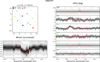 |
Fig. A.3 Same as Fig. 1 but for RJD 60082 and not showing the discarded T3PHI and |V| observables. |
| In the text | |
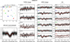 |
Fig. A.4 Same as Fig. 1 but for RJD 60112. |
| In the text | |
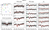 |
Fig. A.5 Same as Fig. 1 but for RJD 60171. |
| In the text | |
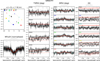 |
Fig. A.6 Same as Fig. 1 but for RJD 60172. |
| In the text | |
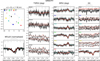 |
Fig. A.7 Same as Fig. 1 but for RJD 60205. |
| In the text | |
Current usage metrics show cumulative count of Article Views (full-text article views including HTML views, PDF and ePub downloads, according to the available data) and Abstracts Views on Vision4Press platform.
Data correspond to usage on the plateform after 2015. The current usage metrics is available 48-96 hours after online publication and is updated daily on week days.
Initial download of the metrics may take a while.