| Issue |
A&A
Volume 699, July 2025
|
|
|---|---|---|
| Article Number | A297 | |
| Number of page(s) | 13 | |
| Section | Astrophysical processes | |
| DOI | https://doi.org/10.1051/0004-6361/202554312 | |
| Published online | 16 July 2025 | |
The geometry of intermittent and magnetospheric state changes pulsars
1
National Astronomical Research Institute of Thailand (Public Organization), 260 M.4, Donkaew, Maerim, Chiang Mai, 50180, Thailand
2
Max Planck Institut für Radioastronomie, Auf dem Hügel 69, D-53121 Bonn, Germany
3
Jodrell Bank Centre for Astrophysics, School of Physics and Astronomy, University of Manchester, Manchester M13 9PL, UK
4
Dept. of Physics and Astronomy, University of British Columbia, 6224, Agricultural Road, Vancouver, B.C., V6T 1Z1, Canada
⋆ Corresponding author: This email address is being protected from spambots. You need JavaScript enabled to view it.
Received:
28
February
2025
Accepted:
16
May
2025
Abstract
Context. Pulsars exhibit a variety of phenomena, including intermittency and magnetospheric state changes (MSC) – moding, nulling, and profile ν˙-correlation – which are thought to be related to changes in their magnetospheric plasma. The variation in pulsar emission patterns has been attributed to changes in the flow of magnetospheric plasma above the polar cap, affecting both radio emission and pulsar spin-down (ν˙).
Aims. This study aims to explore the link between these behaviours by investigating the geometry and spin-down characteristics of intermittent pulsars and MSC pulsars.
Methods. We estimated the magnetic inclination angles for intermittent pulsars and a sample of MSC pulsars using the rotating vector model and pulse-width-period correlations. A ‘plasma filling factor’ was introduced to extend the model proposed by Li et al. (2012b, ApJ, 746, 60) to MSC pulsars, with the aim of providing a unified framework for understanding these phenomena.
Results. Our results provide supporting evidence for a relationship between spin-down ratios and inclination angles that aligns with theoretical predictions. We determine the plasma filling factor explaining the observed spin-down variations for a number of pulsars. We also identify unusual emission height characteristics in PSR B1931+24 that suggest distinctive magnetospheric properties in intermittent pulsars.
Conclusions. This work establishes a quantitative link between intermittent and MSC pulsars through a simple unified model of magnetospheric plasma depletion. Future observations of additional pulsars with known spin-down variations will be crucial for refining this model and deepening our understanding of pulsar magnetospheres.
Key words: pulsars: general
© The Authors 2025
 Open Access article, published by EDP Sciences, under the terms of the Creative Commons Attribution License (https://creativecommons.org/licenses/by/4.0), which permits unrestricted use, distribution, and reproduction in any medium, provided the original work is properly cited.
This article is published in open access under the Subscribe to Open model. This email address is being protected from spambots. You need JavaScript enabled to view it. to support open access publication.
1. Introduction
The occurrence of radio emission in pulsars, produced from accelerated charged particles in the magnetic open-field-line region above the polar cap, has been shown to be closely connected to the pulsar's spin-down ( ) via a braking torque caused by the current of the charged particles (Kramer et al. 2006; hereafter KLO). The connection has been made through the study of intermittent pulsars, which switch between the radio-active (ON) and radio-quiet (OFF) states on timescales of weeks, months, or years. The discovery of this class of pulsars represented by PSR B1931+24 (KLO) was later followed by PSR J1832+0029 (Lorimer et al. 2012) and PSR J1841−0500 (Camilo et al. 2012). Recent spin-down measurements of PSRs J1832+0029 and J1841−0500 have been reported by Wang et al. (2020), finding the rates consistent with those of previous publications. A detailed analysis of two further intermittent pulsars, PSRs J1910+0517 and J1929+1357, was presented by Lyne et al. (2017).
The observation that the  of intermittent pulsars in the OFF state (
 ) is smaller than that of the ON state (
 ) is interpreted such that the pulsars are losing energy more slowly in the OFF state. This is because in the OFF state there is no charge current flow in the open-field-line region, which would add an additional torque and would have otherwise generated the radio emission. This model of KLO, where
  is given by dipolar braking, was later refined by Li et al. (2012a, b) (hereafter, LSTa and LSTb, respectively). Keeping the same ON and OFF definition, their magnetospheric model mostly differed from KLO as it considered the impact of the closed-field-line region. Similarly, the open-field-line region has two states: (1) the ON state, where it is abundantly filled with an outward plasma stream with extremely high conductivity (‘force-free’); and (2) the OFF state, in which the charged particle flow is prohibited, causing the radio emission to cease. For the closed-field-line region, the plasma is similarly abundant in both states. It is understood that outflows of the charged particles create an electric return current, which flows from the light cylinder – the distance where the co-rotating transverse velocity reaches the speed of light – back to the polar cap to complete the ‘circuit’ (e.g. Contopoulos et al. 1999; Philippov & Kramer 2022). This current flow causes a braking torque, in addition to the slowdown caused by magnetic dipole radiation, even if the pulsar is an aligned rotator (see LSTa and references therein). Because the currents depend on the geometry of the magnetic-field lines, LSTa's model predicts a relationship between the change in spin-down rate,
  , and the angle between the rotational and magnetic axis, α. For small α values of an aligned rotator, the spin-down luminosity (L) is smallest in the OFF state, both because the magnetic dipole braking depends on sin α and because the displacement currents are close to zero and the large-scale conduction currents are small; hence open-field lines carry minimal Poynting flux. As α increases, the Poynting flux increases, while the magnetic dipole braking contribution increases as more magnetic flux passes through the light cylinder. Both contributions increase the spin-down luminosity compared to the simple vacuum case. This increase in Poynting flux over the vacuum spin-down luminosity in the OFF state is greatest at high inclination angles, where the open-field lines in the vacuum solutions carry the most Poynting flux. The expected dependence of the spin-down luminosity on the magnetic inclination angle for the ON and OFF states is shown in Figure 1 via solid red and blue lines, respectively. We also show the dependence of the smaller vacuum spin-down luminosity as a solid purple line (see LSTa for details).
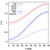 |
Fig. 1. Normalised spin-down luminosity (L) as a function of the magnetic inclination angle, α, as derived by LSTa (see their Figure 3). The solid curves represent three cases: the ON state (red), the OFF state (blue), and the vacuum state (purple). The model assumes a complete absence of plasma in the open-field-line region during the OFF state. In Section 3, we consider a modification of this model when the degree of depletion is less than complete; this is described by a ‘plasma filling factor’, η. Corresponding curves for η = 0.9 (dashed), 0.5 (dotted), and 0.1 (dashed dotted) are shown. See Sections 1 and 3 for details. |
As a result of the above, the relative difference between the ON spin-down and the OFF spin-down becomes smaller as the inclination angle increases. The corresponding spin-down ratio,  , is therefore largest for small α values and smallest for orthogonal rotators (see Figure 8). Reality will almost certainly be more complicated than assumed in this simple model (for a recent review, see Philippov & Kramer 2022), but one aim of this work is to test this relationship against observations.
Another aim of this paper is to consider what happens when a state change in the Poynting flux is associated with a less complete absence of plasma in the open-field-line regions. This follows the work of Lyne et al. (2010) (hereafter LHK), which presented observations of long-term variations in pulsar spin-down and their relationship with profile changes in sources previously considered to be ‘normal’ pulsars. Based on their results, they argued that pulsar intermittency is related to the well-known phenomena of ‘moding’ and ‘nulling’ observed in a number of pulsars (e.g. Wang et al. 2007). While intermittent pulsars switch magnetospheric states on timescales of days, months, and years, the latter group shows state changes in the average pulse profile (moding) or temporary shutdowns of radio emission (nulling) on timescales of seconds to hours (e.g. Lyne & Smith 2004). While it is not yet known what causes these changes in state, LHK's observations suggest that moding and nulling may occur when the amount of plasma (and associated current) in the open-field-line region changes, but is not completely absent, while still affecting the spin-down behaviour. As a striking example, for PSR B1828−11 Stairs et al. (2019) showed a correlation between the fraction of time it spends in each of its modes and observed changes in its spin-down. As pointed out by LHK, partial or complete disruptions or redistributions in the magnetospheric particle supply may not only cause profile changes or nulls, they could also explain some of the pulsar timing noise. This view unifies a variety of pulsar phenomena to have the same – albeit little understood – physical origin.
Brook et al. (2016) analysed 168 pulsar datasets using Gaussian process regression to find a correlation between profile shape and spin-down in previously known sources, including a new case, PSR J1602–5100. They showed that the correlation is clear for some pulsars but not for others, which may indicate a more complex relationship between spin-down and pulse-profile variability, a limitation in the detection of profile variability, and/or the validity of the initial assumption about the timing noise and timing model. In the study by Shaw et al. (2022) (hereafter SSW), the authors provided an update on LHK's findings, detailing a total of 17 pulsars that exhibit notable variations in their spin-down rates, with a subset of eight pulsars showing a correlation between the variation in their  and the corresponding changes in their pulse profiles. Furthermore, both LHK's work and a subsequent analysis by SSW converged on the conclusion that
  exhibits a linear dependence on
  , as
, as  (SSW). In the following, we refer to moding and nulling pulsars and pulsars with long-term profile variations with and without
  correlation as magnetospheric-state-change (MSC) pulsars.
Conspicuously, profile or pulse-shape variations have not yet been reported for intermittent pulsars. Young et al. (2013) analysed a 13-year dataset of PSR B1931+24 from 1998 to 2011 and found no systematic intrinsic variations in the pulse shape during the ON phase. Nevertheless, because of the obvious observational link between intermittent and MSC pulsars, we tried to apply the LSTa model to all these pulsars, focusing on those where a change in spin-down has been measured.
In this paper, we first attempt to provide estimates for the magnetic inclination angle of intermittent and MSC pulsars. We do this via studies of the pulse profile, namely via its polarisation properties and via a statistical argument using its pulse width in Section 2. This allows us to compare the derived values with the observed changes in spin-down rates in Section 3. We modified the LSTa model by introducing a magnetospheric filling factor and applied it to MSC pulsars. In Section 4, we discuss the results and the relationship between intermittent and MSC pulsars.
2. Geometry of intermittent and MSC pulsars
To search for a dependence of the spin-down ratio on the magnetic inclination angle of intermittent and, eventually, MSC pulsars, we need to determine the geometry of these pulsars. The geometry is described by two angles: the magnetic inclination angle, α and the impact parameter, β, describing the smallest angular separation between our line of sight and the magnetic axis. Equivalently, one can use the viewing angle, ζ=α+β, towards the observer. In general, these angles can be determined in two ways. One is to use the polarisation data and fit the rotating vector model (RVM) (Radhakrishnan & Cooke 1969) to the linear polarisation-position-angle (PPA) swing. The second method relies on comparing the observed pulse width with statistical properties of the whole known pulsar population, namely the scaling of the size of the radio beam with the pulse period. While this method is applicable to all pulsars, it requires that the individual pulsar under study is indeed representative of an average pulsar and not an extreme case. We first briefly explain both methods and our way of implementing them before applying them first to intermittent pulsars and then to MSC pulsars; finally, we compare and summarise the results needed for the rest of the paper.
2.1. Methods
2.1.1. Method 1: Geometry from the RVM
According to the RVM, the PPA of the linearly polarised emission, Ψ, is expected to show an S-like swing as a function of pulse phase (or pulse longitude), ϕ. Ψ is determined from the measured Stokes parameters Q and U of the pulsar's emission as  . Following the ‘RVM convention’, the change in PPA (see e.g. Johnston & Kramer 2019 for details) depends on α and ζ (or β) according to
 (1)
(1)
where ϕ0 and Ψ0 denote the pulse phase and the PPA value at the steepest slope of the PPA swing.
In the original RVM model, ϕ0 is expected to fall in the plane defined by the rotational and magnetic axes and the direction to the observer. For a symmetric beam, ϕ0 is therefore also expected to coincide with the profile midpoint. A relativistic correction to this view, introduced by Blaskiewicz et al. (1991), causes a delay between the profile midpoint and ϕ0, as will be discussed later.
The values of α and ζ (or β) can be constrained by fitting the RVM to the observed Ψ(ϕ). It has been shown that the RVM is indeed able to derive the underlying geometry (see e.g. Johnston & Kramer 2019; Desvignes et al. 2019), but the structure of Eq. (1) leads to correlations between α and ζ (or β), whereby the fit then often leads to extreme values of α (i.e. close to 0 or 180°) if the range of longitudes of measured PPA values is limited (e.g. for pulsars with small duty cycles). This has been discussed in some detail in the literature (e.g. Everett & Weisberg 2001), and variations such as using the slope of the RVM curve as an additional constraint have been adopted (e.g. Yao et al. 2022). Extrinsic effects such as interstellar scattering can also affect the observed PPA, altering the inferred geometry.
In this work, we implemented the same fitting procedure as described in Johnston & Kramer (2019), but we remain cautious about results where α is found to be close to 0 or 180 deg. In each such case, we consider arguments and a comparison with the results of the second method described next as to whether the RVM result is justified or should be ignored.
2.1.2. Method 2: Geometry from the pulse width
The second method derives an estimate of the geometry from the observed pulse width, which is determined by the extent of the radio beam and the viewing geometry. Assuming a dipolar geometry and an emission beam that fills the open-field line region centred on the magnetic axis, a relationship between the beam (half) aperture angle, ρ, and the pulse width, W, is given by e.g. Lorimer & Kramer (2005)
 (2)
(2)
Alternatively, one can write (Gil et al. 1984)
 (3)
(3)
If ρ can be estimated independently, these relationships can be used to estimate α and ζ from the measured W. In doing so, one usually chooses to measure the width at an intensity level that aims to measure the full extent of the pulsar beam. As we will do below, an intensity level of 10% is often used, measuring W10.
To estimate ρ, we used the results of previous studies that have shown that there is an apparent correlation between beam radius and pulse period, with larger ρ observed for shorter periods, such that ρ=kP−0.5. Such a relationship is indeed expected for pure dipolar field lines and a filled beam. Note that in such cases, the emission height is related to ρ as ρ≈1.24(rem/10 km)0.5P−0.5 deg, where P is measured in seconds (e.g. Lorimer & Kramer 2005)1. The factor k is found to have a weak dependence on radio frequency. For 1.4 GHz and W10, Venkatraman Krishnan et al. (2019) reviewed previous results and found a range of k = 4.9 to 6.5 deg s0.5. We therefore adopted a value of k = 5.7±0.8 deg s0.5 to search the α−ζ parameter space for pairs that satisfy Eq. (2) given a W10 measured for the pulsars studied here. In each case, the uncertainty of W10 is estimated from the 1-σ (RMS) value of the off-pulse region or the time resolution of the profile, whichever is greater.
In order to obtain estimates for α, prior distributions were selected for α and ζ that were uniform in sin(α) and sin(ζ) between 0 and 180 deg, respectively. The ρprior is normally distributed around the value (5.7±0.8)×P−0.5 deg s0.5, obeying a constraint that our line of sight needs to intersect the emission beam, −ρprior<ζ−α<ρprior. A similar likelihood function was used with χ2=((W10−W(α,ζ,ρ))/ΔW10)2, again with the UltraNest sampler by Buchner (2021). To mitigate the resulting α distribution being bimodal, with a peak in each hemisphere, the fit was run and the statistics calculated separately for 0<α<90 deg and 90<α<180 deg. As can be expected, the results from each hemisphere are consistent. In order to estimate an uncertainty for the derived values, prior to applying the method to real data, we ran a Monte Carlo simulation comparing known input values with the output of this method. A look-up table has been produced which assigns a corresponding uncertainty to the real values (see Appendix A).
2.2. Application to intermittent pulsars
For intermittent pulsars, polarisation data are available for only two pulsars, the PSRs B1931+24 and J1841−0500. Corresponding profiles are shown in Figures 2 and 3, to which both methods can be applied. For three other known intermittent pulsars, PSRs J1832+0029, J1910+0517, and J1929+1357, only total power information can be used and therefore method 2.
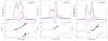 |
Fig. 2. Pulse profiles of PSR B1931+24 at (left) 325 MHz, (middle) 430 MHz, and (right) 1445 MHz, respectively. In each plot, the top panel shows the total (black) and linearly (red) and circularly polarised (blue) intensity. The bottom panels show the position angle of the linearly polarised intensity. Modelling the distinct S-like swing with an RVM results in the red line. The 430 MHz profile is from this work; the 325 MHz and 1445 MHz profile are from Rankin et al. (2023) as obtained from the EPN database (see text for details). |
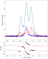 |
Fig. 3. Pulse profile for PSR J1841−0500 as observed by Camilo et al. (2012) at 4.8 GHz. The panels are as for PSR B1931+24 in Figure 2. For the RVM fit, we also display the solution shifted by 90 deg (solid and dashed lines) as this pulsar shows clear orthogonal jumps. |
2.2.1. PSR B1931+24
Figure 2 shows polarisation profiles for PSR B1931+24 at 325, 430, and 1445 MHz. All profiles were observed with the Arecibo 300-m radio telescope. The 325 MHz and 1445 MHz data are taken from (Rankin et al. 2023, hereafter RAN23), available from the EPN database2. The 430 MHz profile is presented here first. It was obtained with the Princeton Mk-IV system in 2001 (Stairs et al. 2000; KLO). Absolute polarisation calibration was not available for the latter. We chose zero longitude to coincide with the pulse peak, consistently in all profiles – a choice we discuss further in Section 4.
A full RVM fit of method 1 was applied to the 325 MHz profile, as this contains the widest range of measured PPAs and the least distortion of the S-like swing. This was done using the UltraNest sampler from Buchner (2021), with priors uniform in sin(α) and sin(ζ) between 0 and 180 deg and using ln(ℒ) = −χ2/2 as the likelihood function (see Johnston & Kramer 2019 for details). The determined solution for the magnetic inclination,  deg, and the viewing angle,
  deg, was held fixed when fitting the 430 MHz and 1445 MHz profiles. For these, the PPA values and the resulting Ψ0 were then adjusted to be consistent with the 325 MHz profile for comparison (i.e. ignoring the effects of Faraday rotation and absolute polarisation calibration). It is noteworthy that the corresponding RVM centroids, ϕ0, are 0.5±0.3 deg at 325 MHz, 1.4±2.0 deg at 430 MHz, and 5.5±1.5 deg at 1445 MHz, relative to the chosen zero longitude. In other words, the delay of the PPA swing is greatest at the highest frequency. We note that this is contrary to what would conventionally be expected, but we refer the reader to Section 4 for further discussion.
To apply method 2, we measured W10 from the 1.4 GHz profile of RAN23 to be 18.0±0.5 deg. Here, we assume that the magnetic axis coincides with the profile peak, chosen as zero longitude, and that the trailing side is weak and only partially visible. To measure the full width of the beam, we therefore took W10 to be twice the width between the leading 10% peak edge and the peak of the pulse. The resulting W10 and those of the following intermittent pulsars are listed in Table 1. The table also lists the magnetic inclination angle derived from method 2, which is  deg.
deg.
Known and determined parameters for intermittent pulsars.
2.2.2. PSR J1841−0500
Polarisation data for J1841−0500 were presented by Camilo et al. (2012) for 2 GHz, 4.8 GHz, and 8.9 GHz (see their Figures 2 and 3). The profiles show a ‘conal core triple component’ (Rankin 1983) configuration and the transition between OPMs at the leading and trailing edges of the central component (e.g. Stinebring et al. 1984). The overall degree of linear polarisation is low, which could attributed to the relatively high observing frequencies (Xilouris et al. 1996). The behaviour at low frequencies is difficult to infer, since the profile is strongly affected by interstellar scattering, even at 2 GHz. The effect of scattering tends to flatten the observed PPA oscillations and thus alters the results of the RVM fitting (Karastergiou 2009). Camilo et al. (2012) therefore attempted to fit the RVM to a subset of their 4.8 GHz data, obtaining constraints α≤45 deg and β≤3 deg (see their Figure 3). For comparison, we fit the RVM to a different subset of their 4.8 GHz data (as shown in their Figure 2). The result of our fit is shown in Figure 3. We did not attempt to fit the 8.9 GHz data, although the effect of the OPMs appears to be less severe. However, this may be due to the lower signal-to-noise ratio, while the degree of polarisation is also low, making a reliable fit difficult. Our derived geometry, α = 155±9 deg and ζ = 156±9 deg, implies a small β and is consistent with the limits presented by Camilo et al. (2012). We note that the RVM centroid, ϕ0=−1.50±0.04 deg, is very well determined, but it precedes the apparent profile midpoint, contrary to what is expected (we refer the reader to Section 4 for further discussion), and scattering in the pulse profile may easily bias the profile midpoint identification. For the same reason, we determined W10 from the 8.9 GHz profile of Camilo et al. (2012). To account for a possible frequency dependence of the pulsar width, we rescaled the width to 1.4 GHz using W10∝f−0.13 (Kijak & Gil 2003). The resulting geometry is listed together with the result of method 1 in Table 1.
2.2.3. J1832+0029, J1910+0517, and J1929+1357
For the intermittent pulsars with the profiles presented in Figures 3 and 4, only total intensity data are available. The profile of PSR B1832+0029 is the result of previously unpublished data spanning a total of 85 hours of data from the Lovell Telescope at 1520 MHz, presented here for the first time. The data were obtained using the Analogue Filter Bank with 64 MHz and a sampling rate of 1 μs (see Hobbs et al. 2004 for details of the observing system). The profiles of PSRs J1910+0517 and J1929+1357 were presented by Lyne et al. (2017). We used the widths measured from these profiles, and the derived geometries are listed in Table 1.
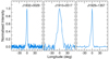 |
Fig. 4. Pulse profiles at 1.52 GHz for further intermittent pulsars J1832+0029 (this work), J1910+0517, and J1929+1357 (both from Lyne et al. 2017), showing total intensity normalised to the pulse peak. |
2.3. Application to MSC pulsars
Figures 5 and 6 show polarisation data for 15 known MSC pulsars. Of these, six pulsars have profile variations (Basu et al. 2024; Johnston et al. 2023), while the remaining nine comprise the sample presented by SSW. The data were obtained with MeerKAT as part of the Thousand Pulsar Array project (see Johnston et al. 2023 for details and data access). For each of these pulsars we used both methods to derive the geometry. The results of the RVM fits are shown in the lower panels of Figures 5 and 6, while Table 2 summarises the results of both methods.
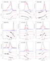 |
Fig. 5. Profiles of MSC pulsars. The corresponding panels are as in Fig. 2. PPA data points that were ignored in the RVM fit are marked in grey. |
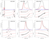 |
Fig. 6. Profiles of MSC pulsars (continued). |
Geometry of MSC pulsars derived using both methods.
We did not consider the RVM results to be reliable for all pulsars. First, PSR J1705−3950 has a broad profile of 38 deg. The pulse shape and the PPA swing show signs of interstellar scattering, which clearly affects both the width measurement and the RVM fit. Second, a number of pulsars with α values close to 0 deg or 180 deg are likely to be affected by the limitations of fitting the RVM in the case of limited PPA ranges, as discussed earlier. Deviations from a simple S-swing at the edges of the PPA range may also limit the effective useful PPA range and thus increase the chance of obtaining extreme αRVM values. For those pulsars, where we consider the αρ−W to be more reliable than the determined αRVM, we present the RVM-related values in Table 2 in parentheses. For four pulsars, we also highlight potential problems with the results derived with method 2 in the same way. We discuss all these cases below.
2.4. Comparing the results of methods 1 and 2
In order to use the most reliable information for the geometry in the rest of the paper, we compare and comment on the results for the pulsars for which both methods were applicable. First, we examine the results for the intermittent pulsars PSRs B1931+24 and J1841−0500.
For PSR B1931+24 we note that the results of both methods are identical, considering that the two solutions α and 180−α cannot be distinguished from each other here. The value for the second method has the smaller estimated uncertainty, i.e.  deg, but both results are consistent with an estimate by RAN23 of 44 deg (no uncertainties given)3. In the rest of this paper we use our value.
For J1841−0500 the results of both methods, αRVM = 155±9 deg and  deg, are also in very good agreement. Both values are also consistent with the constraints presented in Camilo et al. 2012; see Section 2.2.2).
Turning to MSC pulsars, we compare the results listed in Table 2. We find good agreement between the two methods for five pulsars: i.e. J0729−1448, J0742−2822, J1905+0709, J1909+0007, and J2043+2740.4 For five pulsars, PSRs J1121−5444, 1141−3322, J1705−3950, J1820−0427, and J1844+1454, we consider the RVM results of method 1 to be unreliable and continue to use αρ−W from method 2. The remaining five pulsars are discussed next.
For PSR J0922+0638, the results of both methods are questionable. In addition to the limitations of the RVM fit, αρ−W may also be biased since the leading part of the profile appears to be ‘missing’, leading to a classification of the pulse shape as a ‘partial cone’ (e.g. Rankin et al. 2006). We therefore adopted the geometry determined from more sensitive Arecibo observations, i.e. α≈53 deg and ζ≈58 deg (see Rankin et al. 2006).
The αRVM value of PSR J0953+0755 indicates an almost orthogonal geometry, which seems to be supported by the presence of an interpulse. However, the low-level emission present for most of the pulse period suggests a nearly aligned rotator. Previous results in the literature are also contradictory. For example, while Blaskiewicz et al. (1991) found the solution for an aligned rotator, Everett & Weisberg (2001) and Wang et al. (2022) prefer an orthogonal rotator. Since it is also difficult to define both a profile centre and a corresponding width, any αρ−W estimate is also unreliable.
For PSR J1741−3927, the estimates for α between the methods differ by about 36 deg, which is much larger than the estimated uncertainties of about 6 deg. The PPA swing shows evidence of OPMs, which may have affected the RVM fit, but there is no clear reason to question the results. Nevertheless, we note that Johnston et al. (2023) classified this source as non-RVM, so we continued using the αρ−W value.
For PSR J1825−0935, we consider the result of method 1, αRVM, to be reliable, as it is consistent with the presence of an interpulse (even though deviations from a simple RVM-like swing are observed) and previous results (e.g. Backus et al. 2010). αρ−W is smaller, but consistent within the uncertainties.
The polarisation data of PSR J1932+2220 have been studied by many authors using RVM fits. Everett & Weisberg (2001) summarised those results, with the majority (including their own fit) pointing towards α≈35 deg. This is in good agreement with our result of αRVM = 41±8 deg, but smaller than our αρ−W estimate. We consider the latter to be unreliable because, as with PSR J0953+0755, it is difficult to define both a profile centre and a corresponding width.
In summary, two intermittent pulsars and 8 of the 15 MSC pulsars have their magnetic inclination angle estimated by RVM fits. For 15 (3 intermittent and 12 MSC) pulsars, we can use an estimate based on the profile width. For a total of nine pulsars we can directly compare the two estimates, which is done in Figure 7. Overall, the results are remarkably consistent, in particular for the intermittent pulsars.
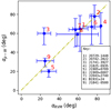 |
Fig. 7. Comparison between resulting αRVM and αρ−W. A dashed yellow-green diagonal line runs from the bottom left to the top right of the plot to represent a 1:1 relationship between the two angles. |
3. Magnetic inclination and spin-down
In the previous section we describe how we derived the magnetic inclination angle, α, of intermittent and MSC pulsars. We used those results to consider a possible relationship between α and the spin-down ratio, R, observed between ON and OFF states for intermittent pulsars. Such a relationship is expected within the LSTa model. Following this, we discuss implications of this model for MSC pulsars.
3.1. Intermittent pulsars
Figure 8 shows  as a function of the magnetic inclination angle as expected in the LSTa model (black line) and its estimated uncertainty (blue band; see the introduction and LSTa for details). We overplot the measured spin-down ratio and our derived α values as listed in Table 1. Note that additional lines labelled with η are discussed in the next section addressing MSC pulsars.
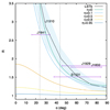 |
Fig. 8. Spin-down ratio, R, as function of determined magnetic inclination angles for intermittent pulsars, PSRs J1832+0029, J1841−0500, J1929+1357, and B1931+24. For PSR J1910+0517, only geometry information is available. These values are compared with the LSTa prediction (black line) and its uncertainty (blue band). In addition, the dependence of the spin-down ratio on α, as predicted by Eq. (7), is plotted for different plasma filling factors: η = 0, 0.1, 0.5, 0.8, and 0.95. |
For PSRs J1841−0500 and B1931+24 there is good agreement between the measurements and the expectations. The inclination angles determined for PSRs J1929+1357 and J1832+0029 appear to be somewhat too high to fit the prediction, but they are still in agreement within their estimated uncertainties. Both values were derived using method 2. Overall, despite the large uncertainties and the limited number of intermittent pulsars, our results seem to support the expected relationship. No published spin-down ratio is available for J1910+0517. If the prediction and our geometry are indeed correct, we would expect to measure a large spin-down ratio of R≈2.5.
3.2. MSC pulsars
In this section, we explore the possible application of the physical ideas behind the LSTa model to MSC pulsars. Following the discussion in LHK and described in the introduction, we assume that profile changes and changes in spin-down for MSC pulsars are associated with similar, but smaller, changes in Poynting flux and current; we therefore expect the observables to also depend on the magnetic inclination angle. By introducing the magnetospheric plasma filling factor, η, we took a heuristic approach and assumed that the degree of plasma depletion in the open-field lines is complete, η = 0, for intermittent pulsars, and less complete, 0<η<1, for MSC pulsars. We also introduced a generalised spin-down ratio,  , which compares the spin-down luminosity for a fully active open-field-line region to one that is partially depleted. Note that we are considering the amount of plasma and Poynting flux in absolute terms, but relatively to normal pulsars (normalised luminosity, as in Figure 1).
In order to derive an expression for Rη, we must first derive an expression for the contribution of the open-field-line region, since it is its plasma content that we wish to modify. We followed LSTa,b and started by considering the spin-down luminosities for the different states shown as the red, blue, and purple lines in Figure 1. For our purposes, these can be adequately described by simple relations given by (see also Spitkovsky 2006 and LSTb)
 (4)
(4)
 (5)
(5)
 (6)
(6)
LSTa,b estimated an uncertainty in their calculation of the order of 10% due to boundary effects and numerical dissipation of the Poynting flux in the magnetosphere (see discussion in LSTa,b for more details). Note that in the OFF state, the Poynting flux due to the plasma component has the strongest α dependent on all three states (see introduction).
With the following considerations, we can use these functional descriptions to identify the parts of the different physical contributions to the total spin-down, which are f(α)Dipole from the magnetic dipole, f(α)Open from the open-field-line region, and f(α)Closed from the closed-field-line region.
We started with the magnetic-dipole contribution, which is identical to that of the vacuum spin-down (Eq. (4)). Therefore, f(α)Dipole = 0.67sin2α.
For the contribution of the closed-field lines, f(α)Closed, we continued on from the notions outlined in the introduction and consider that for intermittent pulsars in the OFF state, the contribution of the open-field lines is missing; hence, f(α)Open = 0, while both magnetic dipole and currents due to plasma in the closed-field lines contribute. In other words, f(α)OFF=f(α)Closed+f(α)Dipole. Using Eq. (6), we therefore identify f(α)Closed=(0.1+1.47sin2α)−(0.67sin2α) = 0.1+0.8sin2α.
In the ON state, the additional Poynting flux due to the plasma component in the open-field-line region, which ultimately causes the radio emission, also contributes; i.e. f(α)ON=f(α)Closed+f(α)Dipole+f(α)Open or, more simply, f(α)ON=f(α)OFF+f(α)Open. Using Eqs. (5) and (6), f(α)Open=f(α)ON−f(α)OFF=(1.0+1.0sin2α)−(0.1+1.47sin2α) = 0.9−0.47sin2α.
In summary, we list the various contributions to the spin-down luminosity in Table 3. Although this separation of contributions is clearly a simplification of the complex, real physical situation and will therefore have its limitations, it does allow us to discuss the physical significance of the three contributing terms. In particular, for the contribution fOpen we have so far assumed that the whole open-field-line region is active. We can now modify this assumption by using the plasma filling factor, η, to derive Rη.
Spin-down luminosity contributions.
We assume that one emission mode of a moding pulsar, or the non-null state of a nulling pulsar, both correspond to the full ON state in an intermittent pulsar, f(α)ON=f(α)Closed+f(α)Dipole+f(α)Open. We also assume that the spin-down in another mode, or during a null, then again has contributions from the dipole, and the closed field line plus the contribution from the Poynting flux of the partially filled open-field-line region, f(α)ON,partial=f(α)Closed+f(α)Dipole+η·f(α)Open. We plot f(α)ON,partial for various η-values in Figure 1 as dashed, dotted, and dashed-dotted lines. As expected, these curves lie between the OFF and the fully ON state.
Following Table 3, we can write
 (7)
(7)
We plot lines for different η values in Figure 8. As can be seen, the corresponding ratios are always smaller than those of intermittent pulsars (see Section 3.1), and we recall that η = 1 corresponds to an always full magnetosphere, while η = 0 represents a completely depleted open-field-line region, as in intermittent pulsars5 This provides a simple tool to explore the implications for moding and nulling pulsars.
Figure 9 shows the variation of η as a function of α. Although the geometry of the intermittent pulsars is known (Table 1), and they all lie on the axis with η = 0, we nevertheless illustrate the relationship between η and α for their specific R values. This is interesting because above the dashed curve drawn for R = 1.28, full depletion of the magnetosphere is apparently not allowed in this model. In other words, as long as some plasma is present in the open-field-line region (η>0), a measured spin-down ratio is bound to be R<1.28, regardless of the magnetic inclination angle. Similarly, for intermittent pulsars we always expect R>1.28, which may allow us to test this simple model in the future.
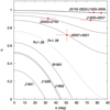 |
Fig. 9. Relationship between η, Rη, and magnetic inclination angle, α, from Eq. (7). We derived η for selected pulsars with measured |

In the same figure, we present the η(α)-curves for the R value of selected pulsars included in the SSW and Young et al. (2012) samples. These are PSRs J0742–2822, J1825–0935, J1909+0007, J2043+2740, and J2037+3621, which have R values of 1.0066, 1.0075, 1.029, 1.061, and 1.12, respectively. As expected, we see the flat α-dependency for a small R. For a given R, a larger depletion (smaller η) is anticipated for a larger α. For example, in the case of PSR B2035+36 (J2037+3621), the difference in the value of η could be as large as ∼40% when comparing α∼90 to α∼0 deg. This illustrates that the switching magnetosphere of a pulsar with large α must be depleted deeper than that of more aligned pulsars to maintain a similar spin-down value.
A simultaneous measurement of R and α can be used to constrain the underlying filling factor. From our work, this is possible for four pulsars, PSRs J0742–2822, J1825–0935, J1909+0007, and J2043+2740, with α measured. In addition, we include PSR J2037+3621 as a fifth pulsar, which has the largest R in SSW, with α = 51±10 deg6 (RAN23). We find that η of those five pulsars are 0.97±0.01, 0.96±0.01, 0.89±0.02, 0.90±0.02, and 0.72±0.06, respectively.
4. Discussion
In Section 2 we present and discuss the geometry measurements for five intermittent pulsars and 15 MSC pulsars using two methods. For nine sources (two intermittent and seven MSC pulsars), we obtained measurements of the magnetic inclination angle with both the RVM and width methods. For five of them, we found good agreement between the methods (including the intermittent pulsars), while for four pulsars we preferred the result of method 2. Overall, this supports the idea that the two methods implemented can indeed be deployed to determine the geometry of radio pulsars.
4.1. General considerations
In total, we determined the geometry for 18 sources using at least one method. This allowed us to search for a possible relationship between the spin-down ratio of intermittent pulsars as expected by the LSTa model. Despite uncertainties and the limited number of intermittent pulsars, the resulting α values for PSRs B1931+24, J1841−0500, J1832+0029, and J1929+1357 support the expected relationship. This suggests that a significant spin-down in the range of 2.0–2.7 can be expected for PSR J1910+0517 once it is observed, testing the model further.
Applying a modified LSTa model to MSC pulsars allowed us to determine the depletion factor, η, for five sources. The values obtained are in the range of 0.72–0.97. These magnitudes may suggest that the changes in moding or nulling pulsars are relatively local to the specific line of sight. In the context of the derived heuristic model, it is easy to understand why the spin-down variations found for MSC pulsars are extremely small, amounting to only a few percent. In turn, a variation of the spin-down ratio with α will also be very small, so we do not expect to be able to measure a dependence of the spin-down ratio on α in future observations of MSC pulsars, since the precision of the α measurements will most likely be insufficient.
4.2. The peculiar case of PSR B1931+24
The heuristic model developed describes the transition from normal to intermittent pulsars as a smooth transition controlled by a single parameter, η. This is unlikely to be true, as other, probably still hidden, variables are almost certainly involved. For example, the timescales for state changes in intermittent pulsars are very different from those in moding or nulling pulsars, ranging from millions of pulsar rotations on the one hand to a few tens of rotations on the other. It is unlikely that η is either the consequence or the cause of these timescales. MSC pulsars such as those discussed in LHK and SSW show very long-term variations and sometimes moding at the same time (e.g. PSR B1828−11, Stairs et al. 2019). One should therefore look for further similarities, or differences, between these groups.
One peculiarity that is noticeable for PSR B1931+24, the first known and best studied intermittent pulsar (KLO), is its profile evolution with frequency. We display the profiles presented in Figure 2 again in Appendix B, Figure B.1, where we show the pulse shapes on top of each other and those with an additional profile at 1.4 GHz by Young et al. (2013). We aligned the profiles as in Figure 2, again choosing the pulse peak as zero longitude.
It can be observed that the pulse profile of B1931+24 has four easily resolvable pulse components, and we label them accordingly in Figure B.1. The pulse peak is consistently identified with the third component at all frequencies, which in itself is unusual. According to conventional wisdom, the profile would evolve from a shape where the central component is strongest at low frequencies to one where the outer components dominate at high frequencies (see, for example, Rankin 1983 and Hassall et al. 2012). Very often, the central component shows some degree of circular polarisation (e.g. Lyne & Smith 2004), which is found here for component 3. The first two components show a weak degree of polarisation, with about 50% linear polarisation, as seen in component 4. Component 4 consists of a weak trailing ‘shoulder’, which appears at all frequencies with the same amplitude relatively to component 3. With increasing frequency, component 2 becomes significantly weaker than components 1 and 3 and is barely resolvable at 1.4 GHz.
We also observe that the apparent centre of the profiles precedes the main peak by about 5 deg of longitude at all frequencies. This suggests a missing part of component 4, or additional components on the trailing side, and it guided our earlier choice of profile centre (see Section 2.2.1). Without these considerations it might be tempting to identify the second component with the location of the magnetic axis, but given the location of the circular polarisation swing we decided on component 3. The agreement of the magnetic inclination angles derived by both methods supports this choice.
In Section 2.2.1 we listed the location of the PPA centroids derived from the RVM fits and found that the PPA swing at the lowest frequency is closer to the profile midpoint that at the higher frequency of 1.4 GHz. We demonstrate this in the lowest panel of Figure B.1 in a different way, by shifting the PAs of 430 and 1440 MHz manually until the overlap with the 325 MHz PPA occurs. We measured shifts that were consistent with the RVM results. A delay between profile midpoint and PPA centroid is expected due to aberration (and retardation) effects; this was introduced as relativistic corrections to the RVM by BCW. As aberration depends on co-rotation speed and hence on the emission height, BCW were the first to point out that the delay can therefore be translated into an estimate for such, rem−BCW=−ΔϕRLC/4. In such an interpretation, the emission heights at 430 MHz and, especially, at 1400 GHz would be significantly larger than that at 327 MHz. Note that the absolute height derived here relies on the BCW model interpretation of the shift (but see also the consistent description by Dyks et al. 2004). The relative PPA shift is, however, independent of the choice of profile midpoint; this suggests that, if the delay is relativistic, the higher frequency comes from a higher altitude.
4.3. Radius-to-frequency mapping, or not
Different emission heights for different radio frequencies is a concept called radius-to-frequency mapping (RFM). It was introduced by Cordes (1978), mainly to explain the narrowing of pulse profiles with increasing frequency, thereby associating low-frequency emission with high-altitude locations and vice versa. The BCW interpretation of the relative PPA shifts between the different frequencies would suggest the opposite. At the same time, the profile width of PSR B1931+24 is almost constant, as shown in Figure B.1. Therefore, the RFM concept seems to be invalid for B1931+24. While this could be specific for B1931+24 (or even intermittent pulsars) we are aware of at least one other example in the literature that has opposite BCW behaviour; i.e. the data presented by Mitra & Li (2004) for PSR B2045−16.
Motivated by this discussion, we also studied the relative location of PPA centroid as measured by the RVM fits for the MSC pulsars. We list their location and the emission heights implied by their delay relative to the profile midpoints in Table 2. Considering only those sources, where we are confident about both the determined PPA centroid and the choice of profile midpoint, we find the emission heights are scattered largely between 100 and 1200 km, with an average value of 400±380 km. This is consistent with normal pulsars compared to those of Kijak & Gil (2003), which used a geometric method based on pulse width measurements to estimate emission heights for normal pulsars, reporting values between approximately 100 and 500 km. Gangadhara & Gupta (2001) analysed PSR B0329+54 using aberration-retardation effects and found emission heights between 160 and 1150 km. We note that we find no correlation between emission height and pulse period.
Interestingly, we also find a number of cases where the determined shift of the PPA centroid relative to the profile midpoint is negative. This would correspond to a negative emission height (as indicated in Table 2) and is not consistent with the BCW model. Despite the limited sample size, this is a relatively high percentage of negative cases, reaching almost 50%, which contrasts with the ∼30% result reported by Johnston et al. (2023). This warrants further investigation, which will be presented in a forthcoming publication (Jaroenjittichai et al., in prep.).
If intermittency, moding, and nulling, and long-term profile evolution are related, then profile changes can also be expected for intermittent pulsars. Young et al. (2013) analysed the relative amplitude between components 1 and 3 over the course of 165 days and found that the amplitude variations are not significant within the mean and uncertainty of 0.69±0.09. Comparing the 1.4 GHz profiles of RAN23 and Young et al. (2013) (Figure B.1), the relative amplitudes of these components appear to be somewhat different; i.e. ∼0.8 versus ∼0.56, respectively. This may indicate that the amplitude has increased from the observation epoch of the Young et al. (2013) profile, which is the average between 1998 and 2011, to the epoch of RAN23 and MJD 58679 (2019). However, the estimated ratio of RAN23's 1.4 profile at ∼0.8 is close to the upper limit of Young et al. (2013) at 0.78. A similar behaviour may have been observed for PSR J1841−0500. The pulse profiles observed by Camilo et al. (2012) also show temporal variations between epochs 2009 and 2011 (their Figure 3). However, the authors acknowledge that such variations could be due to the limited number of pulses and/or the presence of RFI in the dataset.
5. Conclusions
We developed a framework that enables us to establish connections among the characteristics of intermittent and MSC pulsars (i.e. moding and nulling pulsars and profile- -correlation pulsars). Through analysis using both the RVM and pulse-width-period correlations, we established estimates of magnetic inclination angles for these populations. Our key findings can be summarised as follows.
First, for intermittent pulsars, our geometric measurements support the theoretical framework proposed by Li et al. (2012a, b). The derived inclination angles support the predicted relationship with spin-down ratios and the underlying magnetospheric model. This is based on the result for PSRs B1931+24, J1841−0500, J1832+0029, and J1929+1357, where the measured geometries agree with theoretical expectations within uncertainties.
Second, we developed a heuristic model that connects intermittent and MSC pulsars through the introduction of a plasma-filling factor (η). This parameter quantifies the degree of plasma depletion in the open-field-line region, ranging from complete depletion in intermittent pulsars (η = 0) to partial depletion in MSC pulsars (0<η<1). This model consistently predicts that MSC pulsars show smaller spin-down variations compared to intermittent pulsars.
Third, our analysis reveals previously unrecognised patterns in the emission height and frequency evolution of PSR B1931+24, where higher frequency emission appears to originate from higher altitudes – if the PPA delay is due to aberration – contrary to the expectations of traditional radius-to-frequency mapping. Whether the apparent failure of conventional radius-to-frequency mapping or the surprisingly large fraction of MSC pulsars with negative BCW delays is significant will be the subject of future studies.
In summary, our work helps to establish a coherent physical picture linking different pulsar-state-change phenomena, from short-term nulling to long-term interruption. Our framework provides quantitative predictions for the relationships between geometry, plasma conditions, and observable state changes. Further work is needed to learn more about the physical origin of the difference between intermittent and MSC pulsars and the rest of the pulsar population.
Acknowledgments
We would like to thank the reviewer for careful consideration of this manuscript and helpful suggestions. This work is supported by the Fundamental Fund of Thailand Science Research and Innovation (TSRI) through the National Astronomical Research Institute of Thailand (Public Organization) (FFB680072/0269).
In other words, such a period scaling for ρ implies that the emission height is independent of the pulse period. Interestingly, previous results such as Johnston & Kramer (2019) and Posselt et al. (2021) (and references therein) infer W10∝P−0.3, which may suggest a power index other than 0.5 in the ρ-P relation. For our sample of pulsars, all periods are sufficiently close to 1s (with the exception of PSR J1910+0517) to have a significant effect on our results if the index differs from 0.5, so we proceeded with this value.
Their value was derived by following Rankin (1990, 1993) and using combined constraints from the pulse width with Eq. (2) and the steepest gradient of the PPA, (sin(α)/sin(β)).
In the latter case, αρ−W is consistent with both  deg and
  deg.
deg.
It should be noted that the OFF curve in LSTa does not follow the assumed sin2(α) dependence perfectly. These and other uncertainties in our reproduction are reflected in a slight underestimation to LSTa's solution (green and black curves), but still within LSTa's quoted model uncertainty (blue area). The level of uncertainty is approximately 10% at α = 90 deg and increases as α decreases, reaching a factor of approximately two at α = 30 deg. For the inclination angles below 30 deg, the L/L0 ratio exceeds three due to the minimal spin-down of the aligned rotator in the OFF state, and substantial uncertainties persist.
We assume an α uncertainty of 10 deg, because it was not provided by RAN23.
References
- Backus, I., Mitra, D., & Rankin, J. M. 2010, MNRAS, 404, 30 [NASA ADS] [Google Scholar]
- Basu, A., Weltevrede, P., Keith, M. J., et al. 2024, MNRAS, 528, 7458 [Google Scholar]
- Blaskiewicz, M., Cordes, J. M., & Wasserman, I. 1991, ApJ, 370, 643 [Google Scholar]
- Brook, P. R., Karastergiou, A., Johnston, S., et al. 2016, MNRAS, 456, 1374 [Google Scholar]
- Buchner, J. 2021, The Journal of Open Source Software, 6, 3001 [NASA ADS] [CrossRef] [Google Scholar]
- Camilo, F., Ransom, S. M., Chatterjee, S., Johnston, S., & Demorest, P. 2012, ApJ, 746, 63 [Google Scholar]
- Contopoulos, I., Kazanas, D., & Fendt, C. 1999, ApJ, 511, 351 [Google Scholar]
- Cordes, J. M. 1978, ApJ, 222, 1006 [NASA ADS] [CrossRef] [Google Scholar]
- Desvignes, G., Kramer, M., Lee, K., et al. 2019, Science, 365, 1013 [Google Scholar]
- Dyks, J., Rudak, B., & Harding, A. K. 2004, ApJ, 607, 939 [NASA ADS] [CrossRef] [Google Scholar]
- Everett, J. E., & Weisberg, J. M. 2001, ApJ, 553, 341 [NASA ADS] [CrossRef] [Google Scholar]
- Gangadhara, R. T., & Gupta, Y. 2001, ApJ, 555, 31 [NASA ADS] [CrossRef] [Google Scholar]
- Gil, J. A., Gronkowski, P., & Rudnicki, W. 1984, A&A, 132, 312 [Google Scholar]
- Hassall, T. E., Stappers, B. W., Hessels, J. W. T., et al. 2012, A&A, 543, A66 [NASA ADS] [CrossRef] [EDP Sciences] [Google Scholar]
- Hobbs, G., Lyne, A. G., Kramer, M., Martin, C. E., & Jordan, C. 2004, MNRAS, 353, 1311 [NASA ADS] [CrossRef] [Google Scholar]
- Johnston, S., & Kramer, M. 2019, MNRAS, 490, 4565 [NASA ADS] [CrossRef] [Google Scholar]
- Johnston, S., Kramer, M., Karastergiou, A., et al. 2023, MNRAS, 520, 4801 [Google Scholar]
- Karastergiou, A. 2009, MNRAS, 392, L60 [Google Scholar]
- Kijak, J., & Gil, J. 2003, ApJ, 397, 969 [Google Scholar]
- Kramer, M., Lyne, A. G., O’Brien, J. T., Jordan, C. A., & Lorimer, D. R. 2006, Science, 312, 549 [NASA ADS] [CrossRef] [Google Scholar]
- Li, J., Spitkovsky, A., & Tchekhovskoy, A. 2012a, ApJ, 746, L24 [CrossRef] [Google Scholar]
- Li, J., Spitkovsky, A., & Tchekhovskoy, A. 2012b, ApJ, 746, 60 [Google Scholar]
- Lorimer, D. R., & Kramer, M. 2005, Handbook of Pulsar Astronomy (Cambridge: Cambridge University Press) [Google Scholar]
- Lorimer, D. R., Lyne, A. G., McLaughlin, M. A., et al. 2012, ApJ, 758, 141 [NASA ADS] [CrossRef] [Google Scholar]
- Lyne, A. G., & Smith, F. G. 2004, Pulsar Astronomy, 3rd edn. (Cambridge: Cambridge University Press) [Google Scholar]
- Lyne, A., Hobbs, G., Kramer, M., Stairs, I., & Stappers, B. 2010, Science, 329, 408 [NASA ADS] [CrossRef] [Google Scholar]
- Lyne, A. G., Stappers, B. W., Freire, P. C. C., et al. 2017, ApJ, 834, 72 [NASA ADS] [CrossRef] [Google Scholar]
- Mitra, D., & Li, X. H. 2004, A&A, 421, 215 [NASA ADS] [CrossRef] [EDP Sciences] [Google Scholar]
- Philippov, A., & Kramer, M. 2022, Ann. Rev. Astr. Ap., 60, 495 [Google Scholar]
- Posselt, B., Karastergiou, A., Johnston, S., et al. 2021, MNRAS, 508, 4249 [NASA ADS] [CrossRef] [Google Scholar]
- Radhakrishnan, V., & Cooke, D. J. 1969, Astrophys. Lett., 3, 225 [NASA ADS] [Google Scholar]
- Rankin, J. M. 1983, ApJ, 274, 359 [Google Scholar]
- Rankin, J. M. 1990, ApJ, 352, 247 [Google Scholar]
- Rankin, J. M. 1993, ApJ, 405, 285 [Google Scholar]
- Rankin, J. M., Rodriguez, C., & Wright, G. A. E. 2006, MNRAS, 370, 673 [Google Scholar]
- Rankin, J., Wahl, H., Venkataraman, A., & Olszanski, T. 2023, MNRAS, 519, 3872 [Google Scholar]
- Shaw, B., Stappers, B. W., Weltevrede, P., et al. 2022, MNRAS, 513, 5861 [NASA ADS] [CrossRef] [Google Scholar]
- Spitkovsky, A. 2006, ApJ, 648, L51 [Google Scholar]
- Stairs, I. H., Lyne, A. G., Kramer, M., et al. 2019, MNRAS, 485, 3230 [NASA ADS] [CrossRef] [Google Scholar]
- Stairs, I. H., Splaver, E. M., Thorsett, S. E., Nice, D. J., & Taylor, J. H. 2000, MNRAS, 314, 459 [Google Scholar]
- Stinebring, D. R., Cordes, J. M., Rankin, J. M., Weisberg, J. M., & Boriakoff, V. 1984, ApJS, 55, 247 [NASA ADS] [CrossRef] [Google Scholar]
- Venkatraman Krishnan, V., Bailes, M., van Straten, W., et al. 2019, ApJ, 873, L15 [NASA ADS] [CrossRef] [Google Scholar]
- Wang, N., Manchester, R. N., & Johnston, S. 2007, MNRAS, 377, 1383 [Google Scholar]
- Wang, S. Q., Wang, J. B., Hobbs, G., et al. 2020, ApJ, 897, 8 [Google Scholar]
- Wang, Z., Lu, J., Jiang, J., et al. 2022, MNRAS, 517, 5560 [NASA ADS] [CrossRef] [Google Scholar]
- Xilouris, K. M., Kramer, M., Jessner, A., Wielebinski, R., & Timofeev, M. 1996, A&A, 309, 481 [NASA ADS] [Google Scholar]
- Yao, J., Coles, W. A., Manchester, R. N., et al. 2022, ApJ, 939, 75 [Google Scholar]
- Young, N. J., Stappers, B. W., Weltevrede, P., Lyne, A. G., & Kramer, M. 2012, MNRAS, 427, 114 [Google Scholar]
- Young, N. J., Stappers, B. W., Lyne, A. G., et al. 2013, MNRAS, 429, 2569 [Google Scholar]
Appendix A: Lookup table for the ρ-W method
The accuracy of the ρ-W method has been evaluated with synthetic datasets. Monte Carlo simulation was employed to generates 3,000 dummy datasets with uniform distributions of 0<sin(α)<90 deg, −ρ<β<ρ deg and 0.1<P<1 second, where ρ=(5.7±0.8)·P−0.5 deg s0.5. The method is applied to each MC dataset, resulting in an α distribution for which a median is measured. Figure A.1 shows the scattered plots of αtrue vs. αρ−W in black. The results appear to exhibit a systematic lower limit of αρ−W, while above 65 deg, the distribution is considerably more scattered. Furthermore, the y-parameter space is devoid of any data points above 78 deg. This is due to the fact that the resulting α is distributed against the edge limit at 90 deg. This results in the solutions being biased away from the maximum boundary, thereby creating a bias against orthogonal solutions. This is an acceptable consequence, given that orthogonal pulsars typically display emission from two opposing poles, situated at 180 deg separation. The y-axis is divided into 80 bins for the calculation of the median, 16th and 84th percentiles of αρ−W. The calculated median is aligned and consistent with αtrue, in comparison to the line y(x) = x. Despite the scattering, this allows the possibility for the αρ−W values to be corrected using a lookup table. The 80 statistics values are used to create a lookup table for this method, which allows the matched α and ±1σ percentiles to be read from the calculated αρ−W.
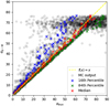 |
Fig. A.1. Comparisons between αρ−W and αtrue (grey points) from the Monte Carlo simulations described in Section 2.2. The Median and ±1σ percentiles are shown in red, blue and green, where the yellow line represents the x=y trend. |
Appendix B: Pulse profiles of PSR B1931+24
Figure B.1 presents a compilation of the intensity and PPA profiles of PSR B1931+24, which are the pulse profiles at 327 MHz (RAN23), 430 MHz (this work), 1.4 GHz (RAN23) and 1.4 GHz (Young et al. 2013), the PPA profiles at 327 MHz (RAN23), 430 MHz (this work), 1.4 GHz (RAN23).
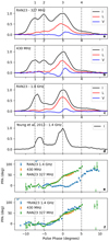 |
Fig. B.1. Compilation of intensity and PPA profiles of PSR B1931+24. (a)-(d) The pulse profiles at 327 MHz (RAN23), 430 MHz (this work), 1.4 GHz (RAN23) and 1.4 GHz (Young et al. 2013). (e) The PPA profiles at 327 MHz (RAN23; green), 430 MHz (this work; orange), 1.4 GHz (RAN23; blue). The intensity and PPA profiles are phase-aligned according to the pulse peak (component 3). (f) Additional phase offset of −1.5 and −5 deg are applied to the 430 MHz and 1.4 GHz PPA profiles in panel (e), respectively. |
All Tables
All Figures
|
Fig. 1. Normalised spin-down luminosity (L) as a function of the magnetic inclination angle, α, as derived by LSTa (see their Figure 3). The solid curves represent three cases: the ON state (red), the OFF state (blue), and the vacuum state (purple). The model assumes a complete absence of plasma in the open-field-line region during the OFF state. In Section 3, we consider a modification of this model when the degree of depletion is less than complete; this is described by a ‘plasma filling factor’, η. Corresponding curves for η = 0.9 (dashed), 0.5 (dotted), and 0.1 (dashed dotted) are shown. See Sections 1 and 3 for details. |
| In the text | |
|
Fig. 2. Pulse profiles of PSR B1931+24 at (left) 325 MHz, (middle) 430 MHz, and (right) 1445 MHz, respectively. In each plot, the top panel shows the total (black) and linearly (red) and circularly polarised (blue) intensity. The bottom panels show the position angle of the linearly polarised intensity. Modelling the distinct S-like swing with an RVM results in the red line. The 430 MHz profile is from this work; the 325 MHz and 1445 MHz profile are from Rankin et al. (2023) as obtained from the EPN database (see text for details). |
| In the text | |
|
Fig. 3. Pulse profile for PSR J1841−0500 as observed by Camilo et al. (2012) at 4.8 GHz. The panels are as for PSR B1931+24 in Figure 2. For the RVM fit, we also display the solution shifted by 90 deg (solid and dashed lines) as this pulsar shows clear orthogonal jumps. |
| In the text | |
|
Fig. 4. Pulse profiles at 1.52 GHz for further intermittent pulsars J1832+0029 (this work), J1910+0517, and J1929+1357 (both from Lyne et al. 2017), showing total intensity normalised to the pulse peak. |
| In the text | |
|
Fig. 5. Profiles of MSC pulsars. The corresponding panels are as in Fig. 2. PPA data points that were ignored in the RVM fit are marked in grey. |
| In the text | |
|
Fig. 6. Profiles of MSC pulsars (continued). |
| In the text | |
|
Fig. 7. Comparison between resulting αRVM and αρ−W. A dashed yellow-green diagonal line runs from the bottom left to the top right of the plot to represent a 1:1 relationship between the two angles. |
| In the text | |
|
Fig. 8. Spin-down ratio, R, as function of determined magnetic inclination angles for intermittent pulsars, PSRs J1832+0029, J1841−0500, J1929+1357, and B1931+24. For PSR J1910+0517, only geometry information is available. These values are compared with the LSTa prediction (black line) and its uncertainty (blue band). In addition, the dependence of the spin-down ratio on α, as predicted by Eq. (7), is plotted for different plasma filling factors: η = 0, 0.1, 0.5, 0.8, and 0.95. |
| In the text | |
|
Fig. 9. Relationship between η, Rη, and magnetic inclination angle, α, from Eq. (7). We derived η for selected pulsars with measured |
| In the text | |
|
Fig. A.1. Comparisons between αρ−W and αtrue (grey points) from the Monte Carlo simulations described in Section 2.2. The Median and ±1σ percentiles are shown in red, blue and green, where the yellow line represents the x=y trend. |
| In the text | |
|
Fig. B.1. Compilation of intensity and PPA profiles of PSR B1931+24. (a)-(d) The pulse profiles at 327 MHz (RAN23), 430 MHz (this work), 1.4 GHz (RAN23) and 1.4 GHz (Young et al. 2013). (e) The PPA profiles at 327 MHz (RAN23; green), 430 MHz (this work; orange), 1.4 GHz (RAN23; blue). The intensity and PPA profiles are phase-aligned according to the pulse peak (component 3). (f) Additional phase offset of −1.5 and −5 deg are applied to the 430 MHz and 1.4 GHz PPA profiles in panel (e), respectively. |
| In the text | |
Current usage metrics show cumulative count of Article Views (full-text article views including HTML views, PDF and ePub downloads, according to the available data) and Abstracts Views on Vision4Press platform.
Data correspond to usage on the plateform after 2015. The current usage metrics is available 48-96 hours after online publication and is updated daily on week days.
Initial download of the metrics may take a while.