| Issue |
A&A
Volume 699, July 2025
|
|
|---|---|---|
| Article Number | A173 | |
| Number of page(s) | 12 | |
| Section | Galactic structure, stellar clusters and populations | |
| DOI | https://doi.org/10.1051/0004-6361/202554305 | |
| Published online | 08 July 2025 | |
Probing the origins
II. Unravelling lithium depletion and stellar motion: Intrinsic stellar properties drive depletion, not kinematics
1
Instituto de Astrofísica, Pontificia Universidad Católica de Chile,
Av. Vicuña Mackenna
4860,
Santiago,
Chile
2
Centro de Astro-Ingeniería, Pontificia Universidad Católica de Chile,
Av. Vicuña Mackenna
4860,
Santiago,
Chile
3
Nicolaus Copernicus Astronomical Center, Polish Academy of Sciences,
ul. Bartycka 18,
00-716,
Warsaw,
Poland
4
INAF – Osservatorio di Astrofisica e Scienza dello Spazio,
Via Gobetti 93/3,
40129
Bologna,
Italy
5
Zentrum für Astronomie der Universität Heidelberg, Landessternwarte,
Königstuhl 12,
69117
Heidelberg,
Germany
6
Max Planck Institute for Astronomy,
Königstuhl 17,
69117
Heidelberg,
Germany
7
Leibniz-Institut für Astrophysik Potsdam (AIP),
An der Sternwarte 16,
14482
Potsdam,
Germany
8
INAF – Osservatorio Astrofisico di Arcetri,
Largo E. Fermi, 5,
50125
Firenze,
Italy
9
Centre for Astrophysics Research, University of Hertfordshire,
College Lane,
Hatfield,
AL10 9AB,
UK
10
Instituto de Astronomia, Geofísica e Ciências Atmosféricas, Universidade de São Paulo,
Rua do Matão 1226,
05508-090
São Paulo,
Brazil
11
Department of Physics & Astronomy, University of North Carolina at Chapel Hill,
NC
27599-3255,
USA
★ Corresponding author: This email address is being protected from spambots. You need JavaScript enabled to view it.
Received:
27
February
2025
Accepted:
21
May
2025
Abstract
Context. Lithium (Li) is a complex yet fragile element, with many production pathways but is easily destroyed in stars. Previous studies observe that the top envelope of the distribution of Li abundances A(Li) in super-solar metallicity dwarf stars shows signs of Li depletion, contrary to expectations. This depletion is thought to result from the interplay between stellar evolution and radial migration.
Aims. In Paper I, we classified a stellar sample from the thin disc with a broad range in metallicity as being churned outwards or inwards, or as stars where angular momentum was preserved (a category including blurred and undisturbed stars, which our method does not separate). In this paper (Paper II), we delve deeper by analysing our entire metallicity-stratified sample along with their dynamic properties, focusing on the connection between radial migration and Li depletion.
Methods. We analysed the chemo-dynamics of a set of 1188 thin-disc dwarf stars observed by the Gaia-ESO survey, previously classified into six metallicity-stratified groups via hierarchical clustering (HC), ranging from metal-poor to super-metal-rich. We examined several features, such as effective temperatures, masses, and dynamic properties. We also implemented a parametric survival analysis using penalised splines (logistic distribution) to quantify how stellar properties and motion (or migration) direction jointly influence Li depletion patterns.
Results. Stars in our sample that seemingly churned outwards are predominantly Li-depleted, regardless of their metallicities. These stars are also the oldest, coldest, and least massive compared to those in the same HC group that either churned inwards or kept their orbital radii. Our survival analysis confirms temperature as the primary driver of Li depletion, followed by metallicity and age, while migration direction shows negligible influence. Additionally, the proportion of outward-churned stars increases with increasing metal-licity, making up more than 90% of our sample in the most metal-rich group.
Conclusions. The increasing proportion of outward-churned stars with higher metallicity (and older ages) indicates their dominant influence on the overall trend observed in the [Fe/H]-A(Li) space for stellar groups with [Fe/H]>0. The survival model reinforces the finding that the observed Li depletion stems primarily from intrinsic stellar properties (cool temperatures, higher metallicity, and old ages) rather than migration history. This suggests the metallicity-dependent depletion pattern emerges through stellar evolution rather than Galactic dynamical processes.
Key words: stars: abundances / Galaxy: abundances / Galaxy: evolution / Galaxy: kinematics and dynamics / Galaxy: stellar content / methods: statistical
© The Authors 2025
 Open Access article, published by EDP Sciences, under the terms of the Creative Commons Attribution License (https://creativecommons.org/licenses/by/4.0), which permits unrestricted use, distribution, and reproduction in any medium, provided the original work is properly cited.
This article is published in open access under the Subscribe to Open model. This email address is being protected from spambots. You need JavaScript enabled to view it. to support open access publication.
1 Introduction
Among all the elements in the Universe, lithium (Li) stands out as one of the most intriguing. It is the third most abundant element produced during the Big Bang nucleosynthesis, and it is also formed shortly thereafter through the decay of beryllium (7Be) into 7Li (e.g. Pinsonneault 1997; Fields et al. 2020). Lithium has diverse production pathways, including nuclear burning in stellar interiors (e.g. in Li-rich giants; see for instance Sackmann & Boothroyd 1992; Sayeed et al. 2024), novae explosions (Starrfield et al. 1978, see also Molaro et al. 2016; Rukeya et al. 2017; Borisov et al. 2024, and references therein), and cosmic-ray spallation (e.g. Olive & Schramm 1992; Knauth et al. 2000). However, Li is a delicate element, making its abundance highly variable. It undergoes significant changes and destruction due to stellar evolutionary processes (e.g. Smiljanic 2020; Randich & Magrini 2021). For instance, the Sun itself has experienced massive Li depletion, losing more than two orders of magnitude in its abundance from the initial value, as recorded in meteorites (Lodders et al. 2009), since the genesis of the Solar System (see e.g. Asplund et al. 2009; Wang et al. 2021, for the current Li abundance).
This complex interplay of production and destruction mechanisms means Li abundances A(Li)s must be interpreted cautiously. The extent of Li depletion is strongly metallicity-dependent: for metal-poor stars ([Fe/H] ≲ −1), the canonical depletion threshold lies near Teff ≃ 5700 K (Rebolo et al. 1988; Romano et al. 1999), whereas solar-metallicity stars require Teff ≳ 6800-6900 K to avoid depletion (Romano et al. 2021). This ~1100 K threshold shift seems to stem from opacity-driven changes in convective structure: higher metal content (particularly Fe and O) increases opacity, deepening convection zones and enhancing Li destruction (Piau & Turck-Chièze 2002, Sect. 3.5 and Table 3). The result resolves the apparent discrepancy between metal-poor halo stars and metal-rich disc populations, demonstrating how metallicity modulates mixing efficiency across Galactic populations.
The absence of detectable star-to-star dispersion in the A(Li)s of warm (Teff ≳ 5700 K), metal-poor (−3 ≤ [Fe/H] ≤-1.5 dex) halo dwarfs has long been interpreted as evidence that those stars display the primordial A(Li) (≃2.1-2.3; e.g. Rebolo et al. 1988; Romano et al. 1999), a conclusion supported also by the measurement of A(Li) ≃ 2.2 in the line of sight to Sk 143, an O-type star in the Small Magellanic Cloud (Molaro et al. 2024). However, the existence of the Li meltdown below [Fe/H] ≃ −3 dex (Sbordone et al. 2010) and the presence of a meagre group of mildly metal-poor halo stars clustering around A(Li) ≃ 2.7 in GALactic Archaeology with HERMES data (GALAH; Gao et al. 2020) underscore the complex interplay between Li survival and stellar parameters (e.g. effective temperature, metallicity, age).
Additionally, rotation-induced mixing is another relevant factor: models by Lagarde et al. (2012) show that a solar-metallicity 1 M star with moderate initial rotation (23% of critical) can deplete Li entirely by 4 Gyr, while a non-rotating counterpart retains its initial abundance. Other models also explore the role of rotation-induced mixing, as well as other stellar properties, in order to estimate the variation of Li in stellar interiors and photospheres (e.g. Deal & Martins 2021). However, we also refer the interested reader to Llorente de Andrés et al. (2021) for a somewhat contrasting discussion on how rotation influences A(Li). Therefore, Li depletion is indeed a multifactorial process.
Several studies have identified signs of Li depletion correlated with increasing metallicity in dwarf stars with super-solar metallicities, i.e. [Fe/H]>0 (e.g. Guiglion et al. 2016; Bensby & Lind 2018; Fu et al. 2018; Grisoni et al. 2019; Bensby et al. 2020). Guiglion et al. (2019) studied a set of old dwarf stars currently inhabiting the solar vicinity with super-solar metallicities and A(Li) below expectations (by comparing with predictions from the models presented by Chiappini 2009, that include prescriptions for Li synthesis in novae outbursts and cosmic ray spallation processes following Romano et al. 1999). Indeed, one would expect metal-rich dwarfs to be formed in regions of complex chemical enrichment histories, such as the inner Galaxy (see also Magrini et al. 2009; Romano et al. 2021). Hence, Guiglion et al. (2019) raised the hypothesis that this phenomenon could be attributed to a combined effect of stellar evolution and radial migration, the latter being responsible for transporting old metal-rich stars from the inner Galaxy to the solar region.
In a previous paper, Dantas et al. (2023), we investigated the behaviour of a set of super-metal-rich stars in the solar neighbourhood that most likely had migrated from the inner regions of the Milky Way (MW); in a follow-up letter, we showed that the stars of our sample with [Fe/H]>0 seem largely Li-depleted (Dantas et al. 2022), confirming that the Li depletion observed in metal-rich stars is likely caused by an interplay between stellar evolution and radial migration. We also argued that the A(Li) in the atmospheres of warm dwarfs (Teff ≲ 6800-6900 K) should not be used as a proxy for the A(Li) in the interstellar medium (ISM), in agreement with Romano et al. (2021). It is worth mentioning that the recent investigation by Llorente de Andrés et al. (2024) has challenged that stellar motion induces Li depletion.
Following the work established in Dantas et al. (2022, 2023), we developed a generalised additive model (GAM; Hastie & Tibshirani 1990) to extend the chemical evolution models computed by Magrini et al. (2009) and use them to estimate the birth Galactocentric radii (Rb) of all the thin disc stars in our sample with varying metallicities, ranging from metal-poor to super-metal-rich (full analysis in Dantas et al. 2025). Therefore, by obtaining both the expected birth radii, Rb, as well as the current guiding radii, Rg, we analysed the motion of the stars in our sample, classifying them as either having been relocated from their original orbital radii (i.e. churned inwards or outwards; this motion is commonly known as radial migration), or having remained approximately at their original orbital radii (i.e. blurred or undisturbed stars).
In this paper, we use the results from Dantas et al. (2025) to better understand the A(Li) of our entire sample while evaluating their stellar motions as well as other critical stellar parameters such as effective temperatures, masses, and ages. The core goals are to (i) evaluate whether the correlation between Li depletion and radial migration entails causation, and (ii) to quantify the relative importance of stellar parameters versus migration history through survival analysis. While we analyse how Li depletion relates to stellar parameters (Teff, [Fe/H], t̄★, as already observed in several earlier studies, such as Deliyannis et al. 1990; Pinsonneault 1997), we do not model depletion mechanisms (e.g. rotation-induced mixing). Instead, we focus on testing whether radial migration itself drives depletion - a hypothesis we ultimately disfavour (see Sect. 3). Our survival modelling approach complements this by rigorously assessing how Teff, [Fe/H], t̄★, and motion direction jointly shape Li survival probabilities. For our sample of stars with [Fe/H] ≳ −1.0, we adopted Teff ≳ 68006900 K as a conservative threshold for identifying objects likely to retain the original Li (see e.g. Gao et al. 2020; Romano et al. 2021), although the Teff range of our sample is below this threshold. In this work, we adopted the solar Li abundance as A(Li) = 0.96 ± 0.05 dex (Wang et al. 2021) and the solar effective temperature as Teff, = 5773 ± 16 K (Asplund et al. 2021).
2 Data and methodology
We used a sample of 1188 thin-disc dwarf stars from the final data release of the Gaia-ESO survey (Gilmore et al. 2012, 2022; Randich et al. 2013, 2022) observed by the Ultraviolet and Visual Echelle Spectrograph (UVES, Dekker et al. 2000), an instrument of ESO’s Very Large Telescope. The atmospheric parameters were derived according to the prescription of Smiljanic et al. (2014) with updates detailed in Worley et al. (2024) and homogenised as described in Hourihane et al. (2023). For age estimations, we used UNIDAM (Mints & Hekker 2017, 2018), a code that uses PARSEC isochrones (Bressan et al. 2012) to estimate stellar ages performing a Bayesian fit using photometric and spectroscopic data from each star. Typical errors are usually around 1 to 2 Gyr (see Mints & Hekker 2017, 2018). For the purposes of this study, it is worth recalling that fast-rotators were removed, meaning we did not account for stars with vsin i > 10 km s−1. This dataset is the same as previously described and analysed in Dantas et al. (2023), and more thoroughly investigated and filtered in Dantas et al. (2025); for the current study, we summarise the data description into its most particular and relevant features.
As detailed in Dantas et al. (2023), we applied quality cuts to ensure the overall reliability of the sample, retaining only stars with RUWE < 1.4, ipd_frac_multi_peak ≤ 2, and ipd_gof_harmonic_amplitude < 0.1, following Fabricius et al. (2021, catalogue validation for Gaia early data release 3, Gaia EDR3). The combination of these flags and thresholds is considered robust for removing contamination by binaries, which could include blue stragglers or blue-stragglers-to-be-objects (see Ryan et al. 2001, for the latter; but see also Kervella et al. 2022 on the identification of binaries through Gaia EDR3). Such binaries could otherwise bias abundances through mass transfer or merger-related Li depletion. We also excluded PECULI-flagged stars (see Hourihane et al. 2023, for the flag definition) from the Gaia-ESO Survey (i.e. removed those with values other than NaN), which include binaries and other peculiar objects.
Among our 1188 stars, 7 lack Li measurements, resulting in a sample of 1181 stars with either detected Li or upper limits. Li estimations for stars observed by Gaia-ESO are described by Franciosini et al. (2022). In this study, we applied the 3D nonlocal thermodynamic equilibrium (NLTE) corrections for A(Li) provided by Wang et al. (2021). Out of our 1181 stars, 13 had lower estimated A(Li) than the grids used in Wang et al. (2021); we chose to keep these corrections anyway and believe potential errors in the overall analysis are small since they affect ~1.1% out of the 1181 stars.
The stars were classified into six metallicity-stratified groups by making use of hierarchical clustering (HC; Murtagh & Contreras 2012; Murtagh & Legendre 2014), which used as input 21 abundances of 18 individual species, as described in Dantas et al. (2022; 2023) and very clearly shown in Dantas et al. (2025, Fig. 1). It should be noted that Li I was not one of the abundances used in the HC. Additionally, we kept the original HC numbering adopted throughout our previous works for consistency. The number of stars in each group and their respective parameters are reported in Table 1, which will be discussed later in the current paper.
In Dantas et al. (2022), we analysed a subset of stars selected from our main sample, focusing only on those with the six highest A(Li) values and super-solar [Fe/H]. The focus on stars with the highest A(Li) values in that work was motivated by the goal of using stars representative of the ISM abundance. However, this is not the case in the current study. Here, we explored the differences and similarities among groups of stars stratified by both metallicity and motion, without limiting the analysis to stars with high A(Li) values. Therefore, in the current study, we examined the entire sample, encompassing stars with a wide range of metallicities, from metal-poor to super-metal-rich.
The detailed description and justification of the survival analysis model are deferred to Sect. 3.2.2, rather than being introduced in this section. This structure ensures that the model’s parametrisation and assumptions are contextualised alongside later empirical findings, as they are informed by insights and discussions developed throughout this manuscript.
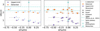 |
Fig. 1 Median lithium abundances (〈A(Li)〉) vs. median metallicity (〈[Fe/H]〉) with their respective median errors for all the stellar groups in our sample, stratified by HC groups and Li detection (orange markers indicate detected values, and purple markers indicate upper limits). Left panel: star-shaped markers depict 〈A(Li)〉 vs 〈[Fe/H]〉 for the entire sample, with each marker annotated to indicate the corresponding HC group. Right panel: similar to the left panel, but further stratified by stellar movement. Circle markers represent stars that moved inwards; x-shaped markers indicate stars that moved outwards; and square markers depict stars with a birth radius similar to their current Galactocentric distance (‘Equal’). In cyan, we additionally display the abundances for the Solar photosphere (⊙), meteorites (⨷), the Spite plateau (horizontal dashed line), and a newer SBBN estimate for A(Li) from Pitrou et al. (2021) at 2.7 dex (horizontal dot-dashed line). Note that upper limits do not include error estimations for lithium since no de facto detection was made, as shown in all other plots of the paper. |
3 Results and discussion
3.1 Confronting stellar parameters with stellar motion
3.1.1 Analysing the complete sample with A(Li) measurements and upper limits
Figure 1 displays two panels with 〈A(Li)〉 vs. 〈[Fe/H]〉 for each HC group, the left one shows the entirety of stars in each group and the right panel depicts each group stratified by motion classes1. In both panels, we include the meteoritic value of A(Li)=3.26 dex (Lodders et al. 2009), which serves as a proxy for the A(Li) of the ISM at the time of the formation of the Solar System; the current solar photospheric abundance [A(Li)=0.96 dex, Wang et al. 2021]; and the Spite plateau as a horizontal dashed line, A(Li)=2.2 dex (Spite & Spite 1982). However, as the Spite plateau does not agree with theoretical expectations, we also include the standard Big Bang nucleosynthesis (SBBN) prediction of ≃2.7 dex (Pitrou et al. 2021), consistent with the 2.6 to 2.8 dex range derived by Cooke (2024) at 95% confidence. We also note that Gao et al. (2020) identified a group of warm stars with [Fe/H] between −1.0 and −0.5 showing a Li plateau at a level consistent with the predictions of SBBN. In addition, Mucciarelli et al. (2022) found a Li plateau in metal-poor giants that, if interpreted taking into account evolutionary mixing processes, is also consistent with SBBN.
In the left panel of Fig. 1, all the HC groups are depicted with star-shaped markers for both detected A(Li) and upper limits (in orange and purple, respectively). The HC group numbers are annotated adjacent to their markers. A mild trend of increasing A(Li) with increasing [Fe/H] up to [Fe/H]=0 is observed, after which the trend inverts, except for the most metal-poor group (HC Group 3), which shows the highest 〈A(Li)〉. The explanation for this higher A(Li) could lie in their overall stellar properties (such as Teff), as we later discuss throughout this paper.
The right panel of Fig. 1 further stratifies the HC groups into motion-classified subgroups. Notably, all the stars in all HC groups classified as having moved outwards underwent significant Li depletion, especially evident for those with detected Li (orange x-shaped markers), but also for those with upper limits.
Figure 2 displays 〈A(Li)〉 vs 〈Teff〉 using the same colours and markers as in the right panel of Fig. 1. The figure clearly shows that different HC groups tend to cluster according to their motion classification, for both detected Li and upper limits. Groups of stars that underwent outwards churning have cooler 〈Teffi〉, which largely explains their depletion. In contrast, those that underwent inward churning, with higher 〈Teff〉, tend to preserve their Li. Groups of stars with unchanged motion (i.e. blurred or undisturbed; represented by the square markers) are located between the inward- and outward-churned groups.
Figures 1 and 2 illustrate the relationship between radial migration and Li depletion: stars that migrated outwards (x-shaped markers) are the coolest in the sample and experienced the most significant Li depletion. Many studies report greater Li depletion in stars with super-solar metallicities (e.g. Guiglion et al. 2016, 2019; Bensby & Lind 2018; Bensby et al. 2020; Stonkute et al. 2020), as these stars predominantly move outwards. In other words, the proportion of metal-rich stars moving outwards is higher than that of metal-poor stars, which affects the overall analysis. By classifying the stars based on different motion classifications, these relationships become evident.
We reinforce that, while complete removal of blue straggler contamination cannot be guaranteed, its impact on our sample seems negligible due to the key observational constraints we described in Sect. 2. Therefore, the majority of the Li-depleted stars in our sample occupy a parameter space distinct from significant blue straggler or blue-straggler-to-be contaminants, which could cause Li depletion due to stellar mergers or mass-transfer.
Our results agree with those of Zhang et al. (2023), who demonstrate that stars migrating outwards show marked Li depletion in the super-solar [Fe/H] regime. However, we extend this analysis by exploring additional stellar parameters, such as Teff, which further contextualise the connection between radial migration and Li depletion, as discussed throughout the current section. Additionally, our results also agree with the findings of Sun et al. (2025), who found that the most Li-rich stars in their sample (comprised of main-sequence turn-off, MSTO, stars) were formed in the outer disc and migrated inwards.
Table 1 presents several parameters for the stars in our sample, categorised by HC group numbers, motion classification, and Li measurements. This table extends Table 3 in Dantas et al. (2025). It is evident that, within each HC group, the stars that underwent Li depletion are the coolest, oldest, and least massive. To better illustrate the relation between 〈A(Li)〉 and age, t̄★, we provide an additional figure (Fig. 3).
To further analyse the effects of age and A(Li) we display in Fig. 3 〈A(Li)〉 vs. t̄★. Distinct markers are placed to distinguish between the different motion classes among the subgroups and different colours to depict the type of Li measurement, similar to Figs. 1 and 2; yet, differently from the previous figures, the solar photosphere and meteorite A(Li)s are displayed in the shape of dot-dashed and dotted cyan lines, respectively. The HC group numbers are annotated adjacent to each marker. It is noticeable that within the same groups, stars churning outwards are systematically the oldest, whereas those churning inwards are the youngest, and those that kept their orbital birth radii (blurred or undisturbed) have systematically intermediate ages.
To verify these correlations, we provide a heat map in Fig. 4, showing these parameters stratified into two panels by Li detection. These correlations are estimated via Spearman’s rank (ρ, Spearman 1904). To gauge these correlations, we assigned arbitrary numerical values to the movement directions: churned outwards (1), churned inwards (−1), or equal motion (0).
Apart from minor differences between the two panels in Fig. 4, which depict the correlations for detected Li and upper limits, respectively, the overall trends among the panels are consistent. Figure 4 confirms expected strong (anti-)correlations, such as those between stellar mass (in solar masses), 〈M〉, and t̄★; as well as between 〈Teff〉 and 〈A(Li)〉. We also find a significant correlation between t̄★ and the direction of motion, especially for stars with upper limits for A(Li) (also observable in Table 1). It is also worth mentioning that no significant (anti-)correlation has been detected regarding eccentricity, 〈e〉, with most of the other parameters, except for angular momentum in the z-direction, 〈Lz〉, which indeed there is a mild correlation; the maximum Galactic height parameter (〈Zmax〉) shows weak anti-correlation with [Fe/H] for stars with detected Li.
Our analysis reveals only a mild anti-correlation between t̄★ and [Fe/H], contrary to the stronger trends typically found in chemically homogeneous samples. This results from our sample’s composition: thin-disc dwarfs spanning a wide metallicity range ( ), originating from distinct Galactic regions with varying star formation histories. As established in Paper I (specifically refer the reader to Fig. 12 in Dantas et al. 2025), the metal-rich population primarily formed in the inner Galaxy, where intense star formation efficiently enriched the ISM. In contrast, metal-poor stars trace the outskirts, where gradual chemical evolution produces weaker age-metallicity coupling. This intrinsic diversity (encoded in the stars’ birth radii) naturally suppresses the global correlation while maintaining coherent sub-population trends.
It is noteworthy that 〈A(Li)〉 and 〈[Fe/H]〉 show no correlation or anti-correlation (ρ = −0.05) for stars with detected Li, but a weak anti-correlation for those with upper limits (ρ = −0.26). This seems to be an effect caused by the choice of using the full sample instead of the stars with the highest A(Li), as previously discussed.
We conclude our discussion of the heat map in Fig. 4 by verifying some of the results from Dantas et al. (2025) not directly tied to A(Li). We observe a mild anti-correlation between 〈Lz〉 and 〈e〉, potentially due to the effects of different stellar motion (churn, blur/lack of disturbance), though this should be treated cautiously as no significant (anti-)correlations are seen between the direction of the movement and 〈e〉, 〈Zmax〉, or 〈Lz〉.
Overall parameters for all the 1180 stars of our sample in order of decreasing 〈[Fe/H]〉 according to their HC group (‘G’).
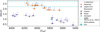 |
Fig. 2 Median lithium abundances (〈A(Li)〉) vs median effective temperatures (〈Teff〉) for all the stellar groups in our sample, stratified by metallicity (through the HC) and Li detection (orange markers indicate detected values, and purple markers indicate upper limits). Circle markers represent stars that moved inwards; X-shaped markers indicate stars that moved outwards; and square markers depict stars with similar birth and current Galactocentric distances (‘Equal’). We additionally display the Sun within this parameter space in cyan (⊙), considering Teff,⊙ = 5773 ± 16 K (Asplund et al. 2021); the Spite plateau can be seen through the horizontal dashed cyan line, as well as the SBBN estimate by Pitrou et al. (2021, dot-dashed line). |
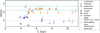 |
Fig. 3 〈A(Li)〉 vs t̄★ for all the stellar groups of our sample with Li measurements. We depict the solar photosphere and meteorite Li abundances in the shape of dotted and dot-dot-dashed cyan lines, respectively. The HC numbers are annotated adjacent to each respective marker. |
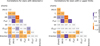 |
Fig. 4 Heat maps displaying the correlations between several parameters for all the stars in the sample stratified by Li detection (detected and upper limits, respectively, from the left to the right). We display the values of 〈[Fe/H]〉, 〈A(Li)〉, t̄★, 〈M〉, 〈Teff〉, 〈e〉, 〈Zmax〉, 〈Lz〉, and direction. We considered direction as a numerical value to classify stars churned either outwards (1) or inwards (−1), and either blurred or undisturbed (0). |
Parameters for the remaining seven stars with missing Li in order of decreasing [Fe/H].
3.1.2 Analysing the stars with missing A(Li)
Beyond our main sample of 1181 stars, we also analysed the 7 stars with missing A(Li). The goal here was to assess whether these stars simply had issues with their Li measurements or if their properties could be consistent with an even stronger Li depletion, which would have potentially impaired their measurements or upper limit estimations. In this case, we display their individual properties in Table 2.
Table 2 shows that all the stars are in the cooler range of the sample, having Teff ≤ 5839 K, which is way below 68006900 K, the estimated threshold of unmodified Li for their high metallicity (Romano et al. 2021, see Sect. 4.1 therein). Five of the seven stars show outward radial migration, while only two remain near their birth radii.
3.2 Survival analysis
3.2.1 Overview of the problem and model reasoning
Selecting an appropriate model to analyse and interpret Li depletion is a challenging endeavour, as it involves a series of assumptions that must be carefully considered in order to reconcile astrophysical expectations with suitable statistical methods. Borrowed from medical research (see, for instance, George et al. 2014; Kartsonaki 2016), survival analysis provides a powerful framework for addressing problems involving censored data in Astrophysics, as discussed in Feigelson & Babu (2012, see their Chapter 10). Censored data arise when the true value of a variable is only partially known - for example, it may be constrained within a range or only known to exceed (or fall below) a given threshold. This situation is common in observational studies, where measurement limitations or design constraints prevent full access to the quantity of interest.
In the context of our study, we encounter three types of Li information: actual measurements, upper limits, and missing values. The latter are likely due to strong depletion, although other factors may be involved, such as when the pipeline was unable to determine Li abundance due to unforeseen issues (e.g. data reduction problems). Statistically, upper limits are typically treated as left-censored observations.
However, our case is somewhat atypical. As established earlier, all stars in our sample likely experienced some level of Li depletion. This is evidenced by both their measured abundances - none approaching the primordial value from SBBN, estimated by Pitrou et al. (2021) at ~2.6-2.8 dex - and by their Teff. In an idealised scenario, stars with Teff ≳ 6800 K and A(Li) close to 2.6 dex could be considered undepleted. Consequently, from a survival analysis perspective, the event of Li depletion has already occurred for all stars in the dataset, making them, in principle, not censored.
Conversely, stars with A(Li) ≳ 2.6 dex would be right-censored, as the event (significant depletion below the primordial value) has not yet taken place: they would still be at ‘risk’. This represents a conceptual shift from the intuitive logic that above a ‘threshold’ means that the event has occurred. In survival analysis terms, we are modelling the drop below a threshold, so stars above it are considered censored because the event is pending.
Nonetheless, adopting 2.6 dex (or other values above it) as a threshold would result in a sample with no censored data, limiting the applicability of survival techniques. For this reason, we instead use a pragmatic threshold corresponding to the Spite plateau (2.2 dex; Spite & Spite 1982), modelling the drop below this value as the event of interest. This allows us to retain censored cases and better capture the depletion process within the sensitivity range of our data. In the following sections, we delve more deeply into the modelling details and the results.
3.2.2 The adopted model
Our analysis employs penalised splines within a parametric logistic survival framework to characterise the non-linear relationships between stellar parameters and A(Li). The model, implemented using the SURVIVAL package (Therneau & Grambsch 2000; Therneau 2024) in the R environment, incorporates P-spline terms with df = 1.5 (degrees of freedom) and penalty constraints for all predictors: t̄★, Teff, [Fe/H], and stellar motion direction (encoded as −1, 0, and +1 for inwardmigrating, non-migrating, and outward-migrating stars, respectively). We explicitly excluded 〈M〉 due to its high collinearity with other parameters (generalised variance inflation factor GVIF1/(2df) > 3 during preliminary testing; see Sect. 3.2.3), which would introduce redundancy without improving model performance. The splines’ adaptive flexibility captures nonlinear trends while the roughness penalty automatically prevents overfitting in data-sparse regions.
The logistic distribution was selected for its dual capacity to model both extreme A(Li) variations and typical abundance regimes. Its heavier tails accommodate chemically peculiar stars with anomalous Li content, while the sharper central peak provides enhanced precision for the bulk population. Crucially, unlike strictly positive distributions such as Weibull or LogNormal (which are suitable for modelling positive response variables, such as time - or ‘survival time’), the logistic framework naturally handles the full dynamical range of observed A(Li) values without artificial truncation.
For the analysis of Li depletion events, the data are classified into four main scenarios. First, for stars with measured A(Li) > 2.2, we consider that a significant depletion event has not yet occurred, so the data are right-censored. In this case, both the upper and lower bounds,  and
and  , are equal to the observed A(Li), reflecting that the star’s Li has not yet dropped below the threshold. Second, for stars with measured A(Li) ≤ 2.2, the event time is exactly known, as A(Li) has already dropped below the threshold (strong depletion is happening). Therefore, both the upper and lower bounds are set to the observed A(Li), and the data are not censored, representing an exact observation. Third, for stars with A(Li) flagged as upper limits, the depletion event has occurred, but the exact timing is uncertain. In this case, the upper bound,
  , is set to the measured upper limit A(Li), while the lower bound,
  , is set to -∞, indicating uncertainty about when the depletion occurred. This scenario is considered interval-censored, as the event has occurred but its exact timing is unknown. Lastly, for stars with missing Li data, we assume that the star is depleted, but the timing of the depletion is uncertain. The upper bound,
  , is set to low_li, which is the smallest observed A(Li) in the entire sample minus 0.05 dex, and the lower bound is set to -∞, reflecting complete uncertainty about when the depletion event took place. This is also treated as interval-censored data. We refer the reader to Table 3 for a summary of the censoring definitions and intervals considered in each type of Li status.
To summarise how each data type is handled in the survival analysis, we classify the observations according to their interpretation and censoring role, which we described above. With this approach, we intend to identify, given the Li status of a star, the factors that determine how far along the depletion process a star is. We then proceed to expose the mathematical representation of the adopted model, which is as follows.
 (1)
(1)
where Yi is the latent survival time [i.e. the log A(Li) at which the threshold crossing occurs], and μi is the linear predictor for the ith star, expressed as a sum of non-linear spline terms:
![Mathematical equation: \mu_i = \beta_0 + f_1(\overline{t}_{{\star},{i}}) + f_2(T_{{\rm eff},i}) + f_3(\text{[Fe/H]}_i) + f_4(\text{direction}_i),](/articles/aa/full_html/2025/07/aa54305-25/aa54305-25-eq12.png) (2)
(2)
where β0 is the model intercept and f1, . . . , f4 denote penalised smoothing splines (P-splines) with 1.5 degrees of freedom, applied to each predictor. These splines transform the raw covariates into flexible, smooth functions that accommodate non-linear dependencies while maintaining computational stability through a quadratic penalty on the second derivatives. The logistic distribution’s parameters - location (μi) and scale (σ) - are thus conditioned on the smoothed predictor space, enabling the model to capture complex relationships without a priori assumptions about functional forms. For our application, the survival function for the logistic distribution is given as
 (3)
(3)
where t represents A(Li) rather than chronological time, and μi is the spline-predicted location parameter for the i-th star. Here, S (t) quantifies the probability that a star’s A(Li) remains above the threshold t (2.2 dex), effectively framing Li depletion as a ‘survival’ process in abundance space. This approach naturally handles the decline of A(Li) while accounting for covariatedependent non-linearities through the spline terms f1, . . . , f4.
Importantly, survival analysis is not the only option for analysing the relation between A(Li) and other variables. Traditional regression techniques remain well-suited to modelling Li as a continuous variable dependent on parameters such as the ones herein used. Our use of survival methods offers an alternative perspective on the depletion process by explicitly modelling threshold crossing.
Censoring definitions for Li depletion events applied in our survival analysis.
3.2.3 Survival analysis results and discussion
The penalised spline regression model achieved exceptional explanatory power for A(Li) variations, with a scale parameter σ = 0.44 indicating highly precise predictions. In logistic survival models, σ represents residual dispersion; values <1 (here 0.44) indicate predictions closely track observations, with σ closer to 0 approaching deterministic relationships. The low σ suggests A(Li) depletion is highly predictable from these parameters, with minimal unmodelled astrophysical scatter.
The deviance statistics (χ2 = 917.66 on 7.59 effective degrees of freedom, p << 0.001)2 further underscore the model’s explanatory strength. Information criteria (AIC = 2047.57, BIC = 2086.13; AIC and BIC corresponding respectively to Akaike and Bayesian Information Criteria; see, respectively, Akaike 1974; Schwarz 1978) validated superiority over alternatives (including Gaussian distributions and unpenalised splines), with lower values indicating better parsimony-adjusted fit (Burnham & Anderson 2002). Collinearity diagnostics confirmed no concerning multicollinearity among predictors, with GVIFs all below 3 [GVIF1/(2df) values: 1.10 (t̄★), 1.06 (Teff), 1.08 ([Fe/H]), 1.09 (direction of motion), well below the conservative threshold of 2.5; see, for instance, Fox & Monette 1992].
Three key trends emerged from the parameter rankings3:
- (i)
Teff dominated as the most influential factor (z = 19.10, p < 2 × 10⁻¹⁶), with positive coefficients (1.08 to 4.24) confirming its protective role: hotter stars retain more Li until saturation above ~6000 K4. The z-value’s magnitude reflects Teff’s overwhelming dominance over other parameters, aligning with its established role in suppressing Li destruction through convective inhibition (e.g. Deal & Martins 2021, see their Figure 4; but see also Piau & Turck-Chièze 2002).
- (ii)
[Fe/H] showed the strongest negative impact (z = −10.36, p < 2 × 10⁻¹⁶), where a 0.1 dex metallicity increase accelerates depletion by 15-20% (derived from exp(−0.54 × 0.1) ≈0.85 to exp(−4.12 × 0.1) ≈ 0.66; i.e. 15-34% faster depletion). We conservatively report 15-20% for typical [Fe/H] ranges. The absolute z-score magnitude confirms metallicity as the secondary driver of depletion, likely through enhanced opacity and mixing (e.g. Piau & Turck-Chièze 2002).
- (iii)
t̄★ exhibited non-linear depletion acceleration after ~2 Gyr (z = −7.75, p = 9 × 10⁻¹⁵), with spline coefficients shifting from −0.15 to −2.25 at this inflection point - aligning with models of deep convection onset (see e.g. Baraffe et al. 2017, and empirical evidence discussed in Carlos et al. 2019; Romano et al. 2021; and Martos et al. 2023, to mention a few).
Motion direction, while considered statistically significant (z = 6.03, p = 1.6 × 10⁻⁹), had negligible practical impact (ΔA(Li) < 0.1 dex, depicting a near-constant trend). The modest z-value relative to intrinsic parameters reinforces that kinematic history is secondary to stellar physics.
The logistic distribution’s heavier tails proved essential for capturing both metal-poor stars with primordial A(Li) and metalrich outliers, a pattern Gaussian assumptions would underestimate. The results for the full survival analysis can be verified in Fig. 5, while the isolated (partial) effects of each parameter to the survival model are depicted in Fig. 6.
This analysis reveals a coherent astrophysical narrative for A(Li) evolution in stars (quantified through full predictions and partial effects in Figs. 5 and 6, respectively): Teff governs the primary survival threshold, metallicity seems to control the efficiency of depletion mechanisms, and t̄★ determines the onset of destructive mixing processes. Crucially, these intrinsic properties seem to operate hierarchically - with Teff setting the initial survival conditions, [Fe/H] modulating the depletion rate, and t̄★ activating late-stage mixing - while kinematic history plays a negligible role. The logistic framework successfully unifies these processes, capturing both the bulk behaviour of A(Li) and the extremes at metal-rich and metal-poor regimes. This supports a paradigm where Li depletion is predominantly driven by the physics of stellar interiors, with Galactic dynamics contributing minimal secondary effects (if at all).
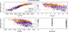 |
Fig. 5 Combined effects of Teff, t̄★, [Fe/H], and direction of motion on the predicted survival time (in this case, the predicted A(Li)), accounting for all covariates simultaneously. Predictions are shown for stars with detected A(Li) measurements (orange), upper limits (purple), and missing A(Li) values (black), with colours consistent across all figures. The curves represent the model’s output from the parametric survival regression (survreg with logistic distribution), integrating the contributions of all covariates. |
4 Summary and conclusions
In this paper, we used a sample of Galactic thin-disc stars retrieved from the final data release of the Gaia-ESO survey. All stars were previously classified into six metallicity-stratified groups via HC, with abundances ranging from super-metal-rich to metal-poor. In Dantas et al. (2025), we used a GAM to extend the MW’s chemical enrichment models described by Magrini et al. (2009) to estimate the probable birth radii of each star in our sample. This allowed us to classify these stars as having churned inwards or outwards (i.e. having suffered radial migration) or as having kept their birth radii (i.e. being either undisturbed or blurred). Using both dynamical classification and parametric survival analysis, we then probed the role of stellar evolution and radial migration in the depletion of Li, as a follow-up to our previous investigation performed in Dantas et al. (2022). Our survival modelling complemented the dynamical approach by quantifying how Teff, [Fe/H], t̄★, and direction of motion (migration or lack thereof) jointly influence Li survival probabilities. We successfully identified the relationship between the A(Li)s and the movement of these stars. Our main conclusions are as follows.
In our sample of FGK-type stars, we observe that those that migrated outwards are typically older, cooler, less massive, and exhibit higher Li depletion when compared to their stellar counterparts that either churned inwards or kept their original orbital radii within each HC group. Most importantly, this result is independent of metallicities (at all ranges). These physical parameters (Teff, [Fe/H], t̄★) are known to be the classical culprits of Li depletion.
On the other hand, the stars in our sample that migrated inwards are generally younger, hotter, and more massive, whereas those that kept their birth orbital radii have intermediate features (i.e. in between outward- and inward-churned stars). With higher temperatures, these stars manage to more efficiently preserve their photospheric Li, because of their thinner convective layers.
Still, the A(Li) of our stellar sample lies systematically below both the meteoritic value and A(Li)max values of younger Gaia-ESO iDR6 open clusters, where undepleted A(Li)s are estimated (Romano et al. 2021). This discrepancy arises because our field stars are predominantly older than 1-2 Gyr, whereas the Gaia-ESO clusters with undepleted Li either contain younger stars (<1 Gyr) or host stars hot enough to preserve their original Li (see Romano et al. 2021, their Table 2). This is strong evidence that all the stars in the current sample suffered Li depletion to some extent.
We provide an assessment of the seven stars with missing Li measurements. Their main features are consistent with a drastic Li depletion, which would explain why it has not been measured in their atmospheres. These stars are also on the cooler side of the sample, with Teff ≤ 5839 K, which is way below the unmodified Li threshold for their metallicity (~ 6800-6900 K, Romano et al. 2021).
Our survival analysis suggests that A(Li) variations across the stellar population may be shaped by three interconnected physical regimes: a temperature-dependent survival threshold, metallicity-driven depletion efficiency, and age-triggered mixing. This tripartite structure tentatively explains both the bulk of the A(Li) distribution and its outliers: from metal-poor stars showing slightly enhanced Li preservation to metal-rich stars exhibiting more rapid depletion. While kinematics appear to play a negligible role in our models, implying predominantly local stellar processes, we caution that minor residual uncertainties (such as small imperfections in NLTE corrections or potential past rotational history effects) could contribute to residual scatter. These findings broadly align with theoretical frameworks of Li evolution in stars (e.g. Somers & Pinsonneault 2015), though we emphasise that our statistical approach complements rather than supersedes existing physical models.
Building on the discussion in Guiglion et al. (2019), Romano et al. (2021), and Dantas et al. (2022), we emphasise that the Li abundance in stars displaying characteristics indicative of potential Li depletion (such as those presented in this study, e.g. Teff ≲ 6800 K) should not be regarded as a reliable indicator of the ISM Li abundance.
The high frequency of Li depletion observed in stars with super-solar metallicities (as shown in earlier studies, such as Delgado Mena et al. 2015; Bensby & Lind 2018; Guiglion et al. 2019; Dantas et al. 2022) emerges naturally from our analysis, especially through the survival regression statistics, as a consequence of three hierarchical stellar properties: Teff (setting the survival threshold), [Fe/H] (modulating depletion efficiency), and t̄★ (activating late-stage mixing). These parameters dominate the observed depletion patterns, particularly in the solar vicinity where metal-rich, outward-migrating stars are overrepresented compared to their metal-poor, inward-migrating counterparts (as shown in Paper I; Dantas et al. 2025).
Our analysis, especially our logistic survival model, demonstrates that the apparent metallicity dependence arises through two complementary mechanisms: (i) the covariance of [Fe/H] with the key depletion drivers (Teff and t̄★), reflecting a selection effect in our sample (likely tied to Gaia-ESO’s target selection; Stonkute et al. 2016); and (ii) the enhanced radiative opacity in metal-rich stars that facilitates Li destruction through deeper convective envelopes. Together, this dual interpretation bridges our statistical results with observational constraints and stellar theory, while agreeing with conclusions from previous studies (e.g. Randich et al. 2020; Charbonnel et al. 2021).
Therefore, the connection between radial migration and Li depletion appears secondary to these intrinsic stellar properties. We theorise that outward churning operates on timescales comparable to stellar evolution, causing outward-migrated stars to exhibit both old ages and characteristic Teff where Li destruction becomes efficient. This explains why the Sun (which most likely migrated from inner Galactocentric distances; see e.g. Tsujimoto & Baba 2020; Dantas et al. 2025) follows the same depletion trend as other cool old metal-rich stars. The survival framework quantitatively supports the following picture: while kinematic history was included as a potential predictor, its negligible contribution in our spline-based model confirms that migration primarily correlates with depletion through its association with temperature, metallicity, and age (the dominant parameters identified in our hierarchical analysis), rather than acting as an independent physical mechanism.
Critically, our analysis demonstrates that the observed correlation between stellar motion and Li depletion does not imply causation: a key distinction, operating through well-characterised stellar physics distinction, that is highlighted throughout this work and supported by the hierarchical dominance of Teff, [Fe/H], and t̄★ in our survival model.
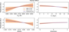 |
Fig. 6 Partial (isolated) effects of Teff, t̄★, [Fe/H], and direction of motion on the predicted survival time (in this case, the predicted A(Li)), derived from a parametric survival model (SURVREG with logistic distribution). Each subplot illustrates the dependence of the predictor on one covariate, while holding all other covariates fixed: Teff, t̄★, and [Fe/H] are set to their mean values to represent central tendencies, while the direction of motion is set to zero as a neutral reference point for directional data. Uncertainty in the partial effects is quantified by 95% (~2σ) and 99% (~3σ) confidence intervals, which account for the flexibility of the penalised splines (PSPLINE) used to model each covariate. |
Data availability
The stellar catalogue and chemo-dynamic parameters used in this work are publicly available through the VizieR service (Ochsenbein 1996) at the Centre de Données astronomiques de Strasbourg (CDS). The specific dataset, originally published in Paper I, can be accessed via DOI: https://doi.org/10.26093/cds/vizier.36960205.
Acknowledgements
The authors thank the referee, Piercarlo Bonifacio, for the kind of suggestions that contributed to the improvement of our manuscript. M.L.L.D. acknowledges Agencia Nacional de Investigación y Desarollo (ANID), Chile, Fondecyt Postdoctorado Folio 3240344. M.L.L.D. and P.B.T. acknowledge ANID Basal Project FB210003. R.S. acknowledges support from the National Science Centre, Poland, project 2019/34/E/ST9/00133. G.G. acknowledges support by Deutsche Forschungs-gemeinschaft (DFG, German Research Foundation) - project-IDs: eBer-22-59652 (GU 2240/1-1 “Galactic Archaeology with Convolutional Neural-Networks: Realising the potential of Gaia and 4MOST”). This project has received funding from the European Research Council (ERC) under the European Union’s Horizon 2020 research and innovation programme (Grant agreement No. 949173). R.S.S. acknowledges the support from the São Paulo Research Foundation under project 2024/053154. P.B.T. thanks Fondecyt Regular 2024/1240465. M.L.L.D. thanks Miuchinha for her long companionship, love, and support. This work made use of the following on-line platforms: slack (https://slack.com/), github (https://github.com/), and overleaf (https://www.overleaf.com/). This work was made with the use of the following python packages (not previously mentioned): matplotlib (Hunter 2007), numpy (Harris et al. 2020), pandas (McKinney 2010), seaborn (Waskom 2021). Based on data products from observations made with ESO Telescopes at the La Silla Paranal Observatory under programme ID 188.B-3002.
References
- Akaike, H. 1974, IEEE Trans. Automat. Control, 19, 716 [Google Scholar]
- Asplund, M., Grevesse, N., Sauval, A. J., & Scott, P. 2009, ARA&A, 47, 481 [NASA ADS] [CrossRef] [Google Scholar]
- Asplund, M., Amarsi, A. M., & Grevesse, N. 2021, A&A, 653, A141 [NASA ADS] [CrossRef] [EDP Sciences] [Google Scholar]
- Baraffe, I., Pratt, J., Goffrey, T., et al. 2017, ApJ, 845, L6 [Google Scholar]
- Bensby, T., & Lind, K. 2018, A&A, 615, A151 [NASA ADS] [CrossRef] [EDP Sciences] [Google Scholar]
- Bensby, T., Feltzing, S., Yee, J. C., et al. 2020, A&A, 634, A130 [NASA ADS] [CrossRef] [EDP Sciences] [Google Scholar]
- Borisov, S., Prantzos, N., & Charbonnel, C. 2024, A&A, 691, A142 [NASA ADS] [CrossRef] [EDP Sciences] [Google Scholar]
- Bressan, A., Marigo, P., Girardi, L., et al. 2012, MNRAS, 427, 127 [NASA ADS] [CrossRef] [Google Scholar]
- Burnham, K., & Anderson, D. 2002, Model Selection and Multimodel Inference: a Practical Information-theoretic Approach (Berlin: Springer Verlag) [Google Scholar]
- Carlos, M., Meléndez, J., Spina, L., et al. 2019, MNRAS, 485, 4052 [Google Scholar]
- Charbonnel, C., Borisov, S., de Laverny, P., & Prantzos, N. 2021, A&A, 649, L10 [NASA ADS] [CrossRef] [EDP Sciences] [Google Scholar]
- Chiappini, C. 2009, IAU Symp., 254, 191 [Google Scholar]
- Cooke, R. 2024, arXiv e-prints [arXiv:2409.06015] [Google Scholar]
- Dantas, M. L. L., Guiglion, G., Smiljanic, R., et al. 2022, A&A, 668, L7 [NASA ADS] [CrossRef] [EDP Sciences] [Google Scholar]
- Dantas, M. L. L., Smiljanic, R., Boesso, R., et al. 2023, A&A, 669, A96 [NASA ADS] [CrossRef] [EDP Sciences] [Google Scholar]
- Dantas, M. L. L., Smiljanic, R., de Souza, R. S., Tissera, P. B., & Magrini, L. 2025, A&A, 696, A205 [NASA ADS] [CrossRef] [EDP Sciences] [Google Scholar]
- Deal, M., & Martins, C. J. A. P. 2021, A&A, 653, A48 [NASA ADS] [CrossRef] [EDP Sciences] [Google Scholar]
- Dekker, H., D’Odorico, S., Kaufer, A., Delabre, B., & Kotzlowski, H. 2000, SPIE Conf. Ser., 4008, 534 [Google Scholar]
- Delgado Mena, E., Bertrán de Lis, S., Adibekyan, V. Z., et al. 2015, A&A, 576, A69 [NASA ADS] [CrossRef] [EDP Sciences] [Google Scholar]
- Deliyannis, C. P., Demarque, P., & Kawaler, S. D. 1990, ApJS, 73, 21 [NASA ADS] [CrossRef] [Google Scholar]
- Fabricius, C., Luri, X., Arenou, F., et al. 2021, A&A, 649, A5 [NASA ADS] [CrossRef] [EDP Sciences] [Google Scholar]
- Feigelson, E., & Babu, G. 2012, Modern Statistical Methods for Astronomy: With R Applications (Cambridge: Cambridge University Press) [CrossRef] [Google Scholar]
- Fields, B. D., Olive, K. A., Yeh, T.-H., & Young, C. 2020, J. Cosmology Astropart. Phys., 2020, 010 [CrossRef] [Google Scholar]
- Fox, J., & Monette, G. 1992, J. Am. Stat. Assoc., 87, 178 [Google Scholar]
- Franciosini, E., Randich, S., de Laverny, P., et al. 2022, A&A, 668, A49 [NASA ADS] [CrossRef] [EDP Sciences] [Google Scholar]
- Fu, X., Romano, D., Bragaglia, A., et al. 2018, A&A, 610, A38 [NASA ADS] [CrossRef] [EDP Sciences] [Google Scholar]
- Gao, X., Lind, K., Amarsi, A. M., et al. 2020, MNRAS, 497, L30 [Google Scholar]
- George, B., Seals, S., & Aban, I. 2014, J. Nucl. Cardiol., 21, 686 [Google Scholar]
- Gilmore, G., Randich, S., Asplund, M., et al. 2012, The Messenger, 147, 25 [NASA ADS] [Google Scholar]
- Gilmore, G., Randich, S., Worley, C. C., et al. 2022, A&A, 666, A120 [NASA ADS] [CrossRef] [EDP Sciences] [Google Scholar]
- Grisoni, V., Matteucci, F., Romano, D., & Fu, X. 2019, MNRAS, 489, 3539 [NASA ADS] [CrossRef] [Google Scholar]
- Guiglion, G., de Laverny, P., Recio-Blanco, A., et al. 2016, A&A, 595, A18 [NASA ADS] [CrossRef] [EDP Sciences] [Google Scholar]
- Guiglion, G., Chiappini, C., Romano, D., et al. 2019, A&A, 623, A99 [NASA ADS] [CrossRef] [EDP Sciences] [Google Scholar]
- Halsey, L. G., Curran-Everett, D., Vowler, S. L., & Drummond, G. B. 2015, Nat. Methods, 12, 179 [Google Scholar]
- Harris, C. R., Millman, K. J., van der Walt, S. J., et al. 2020, Nature, 585, 357 [NASA ADS] [CrossRef] [Google Scholar]
- Hastie, T., & Tibshirani, R. 1990, Generalized Additive Models, Chapman & Hall/CRC Monographs on Statistics & Applied Probability (UK: Taylor & Francis) [Google Scholar]
- Hourihane, A., François, P., Worley, C. C., et al. 2023, A&A, 676, A129 [NASA ADS] [CrossRef] [EDP Sciences] [Google Scholar]
- Hunter, J. D. 2007, Comput. Sci. Eng., 9, 90 [NASA ADS] [CrossRef] [Google Scholar]
- Kartsonaki, C. 2016, Diagnostic Histopathology, 22, 263 [Google Scholar]
- Kervella, P., Arenou, F., & Thévenin, F. 2022, A&A, 657, A7 [NASA ADS] [CrossRef] [EDP Sciences] [Google Scholar]
- Knauth, D. C., Federman, S. R., Lambert, D. L., & Crane, P. 2000, Nature, 405, 656 [Google Scholar]
- Lagarde, N., Decressin, T., Charbonnel, C., et al. 2012, A&A, 543, A108 [NASA ADS] [CrossRef] [EDP Sciences] [Google Scholar]
- Lin, M., Lucas, H. C., & Shmueli, G. 2013, Inf. Syst. Res., 24, 906 [Google Scholar]
- Llorente de Andrés, F., Chavero, C., de la Reza, R., Roca-Fàbrega, S., & Cifuentes, C. 2021, A&A, 654, A137 [NASA ADS] [CrossRef] [EDP Sciences] [Google Scholar]
- Llorente de Andrés, F., de la Reza, R., Cruz, P., et al. 2024, A&A, 684, A28 [NASA ADS] [CrossRef] [EDP Sciences] [Google Scholar]
- Lodders, K., Palme, H., & Gail, H. P. 2009, Landolt Börnstein, 4B, 712 [Google Scholar]
- Magrini, L., Sestito, P., Randich, S., & Galli, D. 2009, A&A, 494, 95 [NASA ADS] [CrossRef] [EDP Sciences] [Google Scholar]
- Martos, G., Meléndez, J., Rathsam, A., & Carvalho Silva, G. 2023, MNRAS, 522, 3217 [NASA ADS] [CrossRef] [Google Scholar]
- McKinney, W. 2010, in Proceedings of the 9th Python in Science Conference, eds. S. van der Walt & J. Millman, 56 [CrossRef] [Google Scholar]
- Mints, A., & Hekker, S. 2017, A&A, 604, A108 [NASA ADS] [CrossRef] [EDP Sciences] [Google Scholar]
- Mints, A., & Hekker, S. 2018, A&A, 618, A54 [NASA ADS] [CrossRef] [EDP Sciences] [Google Scholar]
- Molaro, P., Izzo, L., Mason, E., Bonifacio, P., & Della Valle, M. 2016, MNRAS, 463, L117 [NASA ADS] [CrossRef] [Google Scholar]
- Molaro, P., Bonifacio, P., Cupani, G., & Howk, J. C. 2024, A&A, 690, A38 [NASA ADS] [CrossRef] [EDP Sciences] [Google Scholar]
- Mucciarelli, A., Monaco, L., Bonifacio, P., et al. 2022, A&A, 661, A153 [NASA ADS] [CrossRef] [EDP Sciences] [Google Scholar]
- Murtagh, F., & Contreras, P. 2012, Data Mining and Knowledge Discovery, 2, 86 [Google Scholar]
- Murtagh, F., & Legendre, P. 2014, J. Class., 31, 274 [CrossRef] [Google Scholar]
- Nuzzo, R. 2014, Nature, 506, 150 [Google Scholar]
- Ochsenbein, F. 1996, The VizieR database of astronomical catalogues [Google Scholar]
- Olive, K. A., & Schramm, D. N. 1992, Nature, 360, 439 [Google Scholar]
- Piau, L., & Turck-Chièze, S. 2002, ApJ, 566, 419 [Google Scholar]
- Pinsonneault, M. 1997, Ann. Rev. Astron. Astrophys., 35, 557 [Google Scholar]
- Pitrou, C., Coc, A., Uzan, J.-P., & Vangioni, E. 2021, MNRAS, 502, 2474 [NASA ADS] [CrossRef] [Google Scholar]
- Randich, S., & Magrini, L. 2021, Front. Astron. Space Sci., 8, 6 [NASA ADS] [CrossRef] [Google Scholar]
- Randich, S., Gilmore, G., & Gaia-ESO Consortium 2013, The Messenger, 154, 47 [NASA ADS] [Google Scholar]
- Randich, S., Pasquini, L., Franciosini, E., et al. 2020, A&A, 640, L1 [EDP Sciences] [Google Scholar]
- Randich, S., Gilmore, G., Magrini, L., et al. 2022, A&A, 666, A121 [NASA ADS] [CrossRef] [EDP Sciences] [Google Scholar]
- Rebolo, R., Molaro, P., & Beckman, J. E. 1988, A&A, 192, 192 [NASA ADS] [Google Scholar]
- Romano, D., Matteucci, F., Molaro, P., & Bonifacio, P. 1999, A&A, 352, 117 [NASA ADS] [Google Scholar]
- Romano, D., Magrini, L., Randich, S., et al. 2021, A&A, 653, A72 [NASA ADS] [CrossRef] [EDP Sciences] [Google Scholar]
- Rukeya, R., Lü, G., Wang, Z., & Zhu, C. 2017, PASP, 129, 074201 [NASA ADS] [CrossRef] [Google Scholar]
- Ryan, S. G., Beers, T. C., Kajino, T., & Rosolankova, K. 2001, ApJ, 547, 231 [NASA ADS] [CrossRef] [Google Scholar]
- Sackmann, I. J., & Boothroyd, A. I. 1992, ApJ, 392, L71 [NASA ADS] [CrossRef] [Google Scholar]
- Sayeed, M., Ness, M. K., Montet, B. T., et al. 2024, ApJ, 964, 42 [NASA ADS] [CrossRef] [Google Scholar]
- Sbordone, L., Bonifacio, P., Caffau, E., et al. 2010, A&A, 522, A26 [NASA ADS] [CrossRef] [EDP Sciences] [Google Scholar]
- Schwarz, G. 1978, Annal. Stat., 6, 461 [Google Scholar]
- Smiljanic, R. 2020, Mem. Soc. Astron. Italiana, 91, 142 [NASA ADS] [Google Scholar]
- Smiljanic, R., Korn, A. J., Bergemann, M., et al. 2014, A&A, 570, A122 [NASA ADS] [CrossRef] [EDP Sciences] [Google Scholar]
- Somers, G., & Pinsonneault, M. H. 2015, MNRAS, 449, 4131 [NASA ADS] [CrossRef] [Google Scholar]
- Spearman, C. 1904, Am. J. Psychol., 15, 72 [Google Scholar]
- Spite, F., & Spite, M. 1982, A&A, 115, 357 [NASA ADS] [Google Scholar]
- Starrfield, S., Truran, J. W., Sparks, W. M., & Arnould, M. 1978, ApJ, 222, 600 [NASA ADS] [CrossRef] [Google Scholar]
- Stonkute, E., Koposov, S. E., Howes, L. M., et al. 2016, MNRAS, 460, 1131 [CrossRef] [Google Scholar]
- Stonkute, E., Chorniy, Y., Tautvaisiene, G., et al. 2020, AJ, 159, 90 [Google Scholar]
- Sun, T., Bi, S., Chen, X., et al. 2025, MNRAS, 536, 462 [Google Scholar]
- Therneau, T., & Grambsch, P. 2000, Modeling Survival Data: Extending the Cox Model (New York: Springer) [CrossRef] [Google Scholar]
- Therneau, T. M. 2024, A Package for Survival Analysis in R, r package version 3.8-3 [Google Scholar]
- Tsujimoto, T., & Baba, J. 2020, ApJ, 904, 137 [Google Scholar]
- Wang, E. X., Nordlander, T., Asplund, M., et al. 2021, MNRAS, 500, 2159 [Google Scholar]
- Waskom, M. L. 2021, J. Open Source Softw., 6, 3021 [CrossRef] [Google Scholar]
- Wasserstein, R. L., & Lazar, N. A. 2016, Am. Stat., 70, 129 [Google Scholar]
- Worley, C. C., Smiljanic, R., Magrini, L., et al. 2024, A&A, 684, A148 [NASA ADS] [CrossRef] [EDP Sciences] [Google Scholar]
- Zhang, H., Chen, Y., Zhao, G., et al. 2023, MNRAS, 520, 4815 [NASA ADS] [CrossRef] [Google Scholar]
All parameters used here are presented as median values, derived through previously bootstrapping this sample to estimate uncertainties (see Dantas et al. 2023, for further details).
We interpret p-values cautiously given their well-documented limitations (e.g. Lin et al. 2013; Nuzzo 2014; Halsey et al. 2015; Wasserstein & Lazar 2016), prioritising effect sizes and information criteria as more reliable evidence.
The z-score (z = Coefficient/Std. Error) measures each predictor’s relative importance in driving A(Li) variations. Larger absolute values (|z|) indicate stronger empirical evidence for the parameter’s influence, allowing hierarchical ranking: for example, |z| = 19.10 (Teff) implies 3X greater impact than |z| = 6.03 (direction of motion).
These Teff results are specific to our stellar sample, which lacks hotter stars (Teff & 6800 K) that typically preserve Li more efficiently, as discussed earlier (Sect. 1).
All Tables
Overall parameters for all the 1180 stars of our sample in order of decreasing 〈[Fe/H]〉 according to their HC group (‘G’).
Parameters for the remaining seven stars with missing Li in order of decreasing [Fe/H].
All Figures
|
Fig. 1 Median lithium abundances (〈A(Li)〉) vs. median metallicity (〈[Fe/H]〉) with their respective median errors for all the stellar groups in our sample, stratified by HC groups and Li detection (orange markers indicate detected values, and purple markers indicate upper limits). Left panel: star-shaped markers depict 〈A(Li)〉 vs 〈[Fe/H]〉 for the entire sample, with each marker annotated to indicate the corresponding HC group. Right panel: similar to the left panel, but further stratified by stellar movement. Circle markers represent stars that moved inwards; x-shaped markers indicate stars that moved outwards; and square markers depict stars with a birth radius similar to their current Galactocentric distance (‘Equal’). In cyan, we additionally display the abundances for the Solar photosphere (⊙), meteorites (⨷), the Spite plateau (horizontal dashed line), and a newer SBBN estimate for A(Li) from Pitrou et al. (2021) at 2.7 dex (horizontal dot-dashed line). Note that upper limits do not include error estimations for lithium since no de facto detection was made, as shown in all other plots of the paper. |
| In the text | |
|
Fig. 2 Median lithium abundances (〈A(Li)〉) vs median effective temperatures (〈Teff〉) for all the stellar groups in our sample, stratified by metallicity (through the HC) and Li detection (orange markers indicate detected values, and purple markers indicate upper limits). Circle markers represent stars that moved inwards; X-shaped markers indicate stars that moved outwards; and square markers depict stars with similar birth and current Galactocentric distances (‘Equal’). We additionally display the Sun within this parameter space in cyan (⊙), considering Teff,⊙ = 5773 ± 16 K (Asplund et al. 2021); the Spite plateau can be seen through the horizontal dashed cyan line, as well as the SBBN estimate by Pitrou et al. (2021, dot-dashed line). |
| In the text | |
|
Fig. 3 〈A(Li)〉 vs t̄★ for all the stellar groups of our sample with Li measurements. We depict the solar photosphere and meteorite Li abundances in the shape of dotted and dot-dot-dashed cyan lines, respectively. The HC numbers are annotated adjacent to each respective marker. |
| In the text | |
|
Fig. 4 Heat maps displaying the correlations between several parameters for all the stars in the sample stratified by Li detection (detected and upper limits, respectively, from the left to the right). We display the values of 〈[Fe/H]〉, 〈A(Li)〉, t̄★, 〈M〉, 〈Teff〉, 〈e〉, 〈Zmax〉, 〈Lz〉, and direction. We considered direction as a numerical value to classify stars churned either outwards (1) or inwards (−1), and either blurred or undisturbed (0). |
| In the text | |
|
Fig. 5 Combined effects of Teff, t̄★, [Fe/H], and direction of motion on the predicted survival time (in this case, the predicted A(Li)), accounting for all covariates simultaneously. Predictions are shown for stars with detected A(Li) measurements (orange), upper limits (purple), and missing A(Li) values (black), with colours consistent across all figures. The curves represent the model’s output from the parametric survival regression (survreg with logistic distribution), integrating the contributions of all covariates. |
| In the text | |
|
Fig. 6 Partial (isolated) effects of Teff, t̄★, [Fe/H], and direction of motion on the predicted survival time (in this case, the predicted A(Li)), derived from a parametric survival model (SURVREG with logistic distribution). Each subplot illustrates the dependence of the predictor on one covariate, while holding all other covariates fixed: Teff, t̄★, and [Fe/H] are set to their mean values to represent central tendencies, while the direction of motion is set to zero as a neutral reference point for directional data. Uncertainty in the partial effects is quantified by 95% (~2σ) and 99% (~3σ) confidence intervals, which account for the flexibility of the penalised splines (PSPLINE) used to model each covariate. |
| In the text | |
Current usage metrics show cumulative count of Article Views (full-text article views including HTML views, PDF and ePub downloads, according to the available data) and Abstracts Views on Vision4Press platform.
Data correspond to usage on the plateform after 2015. The current usage metrics is available 48-96 hours after online publication and is updated daily on week days.
Initial download of the metrics may take a while.