| Issue |
A&A
Volume 699, July 2025
|
|
|---|---|---|
| Article Number | A171 | |
| Number of page(s) | 12 | |
| Section | Stellar structure and evolution | |
| DOI | https://doi.org/10.1051/0004-6361/202554264 | |
| Published online | 07 July 2025 | |
Unevolved Li-rich stars at low metallicity: A possible formation pathway through novae
1
Astronomisches Rechen-Institut, Zentrum für Astronomie der Universität Heidelberg, Mönchhofstraße 12-14, 69120 Heidelberg, Germany
2
Institute of Astronomy (IvS), KU Leuven, Celestijnenlaan 200D, 3001, Leuven, Belgium
3
Center for Information Science, Fukui Prefectural University, 4-1-1 Matsuoka Kenjojima, Eiheiji-cho, Fukui 910-1195, Japan
4
Department of Astronomy, California Institute of Technology, 1200 East California Boulevard, Pasadena, CA 91125, USA
5
Department of Physics and Astronomy, University of California, Los Angeles, CA 90095, USA
6
Kapteyn Astronomical Institute, University of Groningen, Landleven 12, 9747 AD Groningen, The Netherlands
7
CAS Key Laboratory of Optical Astronomy, National Astronomical Observatories, Beijing 100101, China
8
School of Astronomy and Space Science, University of Chinese Academy of Sciences, Beijing 100049, China ;
Institute for Computational Cosmology, Department of Physics, Durham University, South Road, Durham DH1 3LE, UK
⋆ Corresponding author: matsuno@uni-heideberg.de
Received:
25
February
2025
Accepted:
14
May
2025
A small fraction of low-mass stars have been found to have anomalously high Li abundances. Although it has been suggested that mixing during the red giant branch phase can lead to Li production, this method of intrinsic Li production cannot explain Li-rich stars that have not yet undergone the first dredge-up. To obtain clues about the origin of such stars, we present a detailed chemical abundance analysis of four unevolved Li-rich stars with −2.1<[Fe/H]<−1.3 and 2.9<A(Li)<3.6, 0.7−1.4 dex higher Li abundances than the ones of typical unevolved metal-poor stars. One of the stars, Gaia DR3 6334970766103389824 (D25_6334), was serendipitously found in the stellar stream ED-3. The other three stars have been reported to have massive (M≳1.3 M⊙) nonluminous companions. We show that three of the four stars exhibit abundance patterns similar to the ones of known unevolved Li-rich stars, namely normal abundances in most elements except for Li and Na. These abundance similarities suggest a common origin for the unevolved Li-rich stars and low-mass metal-poor stars with massive compact companions. We also made the first detection of N abundance to unevolved Li-rich stars in D25_6334, and found that it is significantly enhanced ([N/Fe] = 1.3). The observed abundance pattern of D25_6334, spanning from C to Si, indicates that its surface has been polluted by a former intermediate-mass companion star or a nova system that involves a massive ONe white dwarf. Using a population synthesis model, we show that the nova scenario can lead to the observed level of Li enhancement and also provide an explanation for Li-rich stars without companions and those with massive compact companions.
Key words: stars: abundances / binaries: general / stars: Population II
© The Authors 2025
 Open Access article, published by EDP Sciences, under the terms of the Creative Commons Attribution License (https://creativecommons.org/licenses/by/4.0), which permits unrestricted use, distribution, and reproduction in any medium, provided the original work is properly cited.
This article is published in open access under the Subscribe to Open model. Subscribe to A&A to support open access publication.
1. Introduction
Lithium provides a unique window into the evolution and structure of low-mass stars. It is quickly destroyed at temperatures above ∼2.5×10⁶ K, which can easily be reached in stellar interiors. This results in a significant decrease in surface Li abundance of low-mass stars at the first dredge-up, when they develop a deep convective envelope that mixes the Li-depleted material from the interior to the surface. However, it has been known for more than four decades that a small fraction of low-mass red giant branch (RGB) stars show an enormous Li abundance and are called Li-rich giants (Wallerstein & Sneden 1982). Thanks to large spectroscopic surveys and the precise identification of their evolutionary status from asteroseismology, our understanding of the origin of such Li-rich giants has improved significantly in recent years (Silva Aguirre et al. 2014; Jofré et al. 2015a; Casey et al. 2016, 2019; Smiljanic et al. 2018; Singh et al. 2019, 2021; Kumar et al. 2020; Yan et al. 2021; Deepak & Lambert 2021; Martell et al. 2021; Zhou et al. 2022; Mallick et al. 2023; Tayar et al. 2023; Castro-Tapia et al. 2024). Theoretical efforts have also been made to explain the origin of enhanced lithium in evolved Li-rich stars (Cameron & Fowler 1971; Zhang et al. 2020; Schwab 2020; Mori et al. 2021; Gao et al. 2022; Denissenkov et al. 2024; Li et al. 2023). Thanks to these studies, we now know that the evolutionary phase near the red clump plays a role in producing most Li-rich stars, although it alone cannot explain all the observed Li-rich giants.
In more recent years, some Li-rich stars have also been found among unevolved stars, which have not yet undergone the first dredge-up. Such unevolved Li-rich stars are extremely rare (fewer than ten stars have been confirmed to be Li-rich from high-resolution spectroscopy), but found at low metallicity ([Fe/H] <−1.0) in the field (Li et al. 2018, hereafter L18) and globular clusters (Koch et al. 2011; Monaco et al. 2012), and at solar metallicity (Deliyannis et al. 2002; Yan et al. 2022). We focus on metal-poor unevolved Li-rich stars in this study as their Li enhancements can clearly be identified thanks the almost constant Li abundance of typical metal-poor stars (Spite & Spite 1982a, b; Charbonnel & Primas 2005)1. Their Li abundances exceed the prediction from the standard Big Bang nucleosynthesis (e.g., Coc et al. 2002; Cyburt et al. 2016), requiring the excess Li to be produced somewhere else. As they are unevolved, the Li excess cannot be explained by intrinsic nucleosynthesis and post first dredge-up mixing, making them the most challenging class of Li-rich stars to explain. Hence, pollution from an external source is discussed as a possible origin of the Li-rich stars in the literature (e.g., Koch et al. 2011; Li et al. 2018). The external source could be planets, highly evolved RGB or asymptotic giant branch (AGB) companions, or novae (L18). Better characterizing these unevolved Li-rich stars and enlarging the existing sample are of great interest to constrain their origin. This would then provide insights into the synthesis of Li in the Universe, which is still not fully understood.
Here, we report the discovery of an unevolved Li-rich metal-poor star, Gaia DR3 6334970766103389824 (hereafter D25_6334). This star was identified as a member of the stellar stream ED-3 from its kinematics (Dodd et al. 2023) and selected as a target for follow-up high-resolution spectroscopy, to study the stream's progenitor (Dodd et al. 2025, hereafter D25). The star has an effective temperature (Teff) of 6417 K and surface gravity (log g) of 4.27, and our high-resolution spectroscopic observation reveals it to be a metal-poor star with [Fe/H]=−2.1 and an extremely high Li abundance of A(Li) = 3.5, which is approximately 1.3 dex higher than in typical unevolved metal-poor stars (e.g., Charbonnel & Primas 2005). We report the detailed abundance pattern of the star, including the first measurement of N and Al abundances for an unevolved Li-rich star, to discuss its possible origins.
We complement this discovery with a detailed abundance analysis of three metal-poor main-sequence turn-off stars from El-Badry et al. (2024a, hereafter E24). These stars are identified as having massive, nonluminous companions, which are candidates for neutron stars. Interestingly, all three metal-poor stars with [Fe/H]<−1 in E24 were reported to be Li-rich, which might suggest a possible link between the unevolved Li-rich stars and the metal-poor stars with massive compact companions. While one of the stars, Gaia DR3 6328149636482597888 (hereafter E24_6328), has been extensively studied in El-Badry et al. (2024b), the other two stars, Gaia DR3 1350295047363872512 and 5136025521527939072 (hereafter E24_1350 and E24_5136), have not been subjected to detailed abundance analysis before now. We investigate the link between these three stars with massive compact companions and the previously identified unevolved Li-rich stars by comparing their abundance patterns and discuss if they can be explained by a common scenario.
This paper is organized as follows. In Sections 2 and 3, we describe the data and analysis of the spectra, respectively. After presenting the results in Section 4, we discuss the possible origin of unevolved Li-rich stars in Section 5. We then conclude in Section 6.
2. Data
D25_6334 was identified as a member of the stellar stream ED-3 from its kinematics and followed up with the Ultraviolet and Visual Echelle Spectrograph (UVES; Dekker et al. 2000) of the Very Large Telescope (program ID: 0111.D-0263(A), P.I. E. Dodd). The spectrum was obtained with one of the standard setups of UVES, which covers the wavelength range from 328 nm to 683 nm with a resolving power of about 55 000. We used the phase 3 product for further analysis. We have also used another archival spectrum of the same star obtained with the same instrument one year earlier by Ceccarelli et al. (2024) under the program ID 0109.B-0522(B) to check for radial velocity variation.
We analyzed the high-resolution spectra used by E24 for the three stars; the spectrum of E24_1350 was obtained with the High Resolution Echelle Spectrometer (HIRES; Vogt et al. 1994) on the Keck I telescope, that of E24_6328 was obtained with the Magellan Inamori Kyocera Echelle (MIKE; Bernstein et al. 2003) on the Magellan Clay telescope, and that of E24_5136 was obtained with the Tillinghast Reflector Echelle Spectrograph (TRES; Fürész 2008) on the 1.5 m Tillinghast telescope. The spectral resolutions of the instruments are R∼55 000, 40 000–55 000, and 44 000, and the wavelength coverages are 365–800 nm, 385–910 nm, and 333–967 nm, respectively. Readers are referred to E24 for the details of the observations and data reduction. Note that while these spectra cover a wider wavelength range in the red region than the UVES spectrum, we only analyzed the region that is in common with the UVES spectrum (328–683 nm) for consistency.
3. Analysis
The analysis mostly follows the method described in D25. Below we summarize the analysis and describe differences. We performed the abundance analysis primarily with MOOG (Sneden 1973), a spectral synthesis code under one-dimensional, local thermodynamic equilibrium (LTE) assumptions, unless otherwise specified. For D25_6334, the stellar parameters were estimated from the Gaia and 2MASS photometry using the color-Teff relation of Mucciarelli et al. (2021), the bolometric correction of Casagrande & VandenBerg (2014), and the extinction map of Lallement et al. (2022). The microturbulent velocity (ξ) was estimated by minimizing the trend between Fe abundances derived from individual Fe I lines and their reduced equivalent widths. We also validated the Teff with a spectroscopic method based on a differential abundance analysis using the Python package q2 (Ramírez et al. 2014). It utilizes the excitation equilibrium of Fe I lines, using HD84937 as the reference star, for which we adopted Teff = 6356 K (Heiter et al. 2015), log g = 4.13 (Giribaldi et al. 2021), ξ = 1.39 km s−1 (Jofré et al. 2015b), and [Fe/H]=−1.97 (Amarsi et al. 2022). We also confirmed that the Hα wings are consistent with Teff∼6400 K using the grid of synthetic spectra from Amarsi et al. (2018)2. The Teff and log g for the E24 stars were taken from E24 but the microturbulent velocity and metallicity were rederived by the same method as for D25_6334.
Abundances were derived from equivalent widths for Fe and spectral synthesis for Li, C, N, Na, Mg, Al, Si, Mn, Cu, Sr, Y, and Ba, La, and Eu, with hyperfine structure splitting considered for Na, Al, Mn, Ba, and Eu. For the Li lines, we analyzed both 6104 and 6708 Å lines and used interpolated 3D non-LTE synthetic spectra from BREIDABLIK (Wang et al. 2021, 2024) instead of MOOG. Abundances of Na and Al were corrected for non-LTE effects using the grid of Lind et al. (2022). Table 1 summarizes measured stellar parameters and abundances of key elements as well as the properties of the star, and the abundances of the three stars from E24 are summarized in Table 2. The complete information on the linelist and abundances other than the ones reported in Table 1 are provided in D25.
The property of D25_6334.
The abundances of E24_6328 have been reported in El-Badry et al. (2024b). We confirm that our abundance measurements are largely consistent with theirs; for 17 elements in common, the mean difference is 0.05 dex in [X/Fe] with a standard deviation of 0.15 dex. A notable difference is found for a few elements, namely Na, Co, and Eu. Our Na abundance is significantly lower ([Na/Fe] = 0.00) than theirs ([Na/Fe] = 0.24), which could partly be due to the non-LTE correction of 0.11 dex applied in this study. The Co abundance in this study is based on just one line; thus, the abundance is less reliable than the other elements. The largest difference is seen in Eu abundance; our Eu abundance is higher ([Eu/Fe] = 0.49) than El-Badry et al. (2024b) ([Eu/Fe] = 0.09). This difference is likely due to the inclusion of a weak Eu line at 6645 Å in their analysis, which we do not consider a detectable line. The abundance pattern of E24_6328 is now more consistent with the r-process-dominated pattern of neutron-capture elements. This is more common in metal-poor stars without significant enhancements in s-process elements, such as Ba and La.
The radial velocity of D25_6334 was measured during the abundance analysis by comparing the observed wavelengths of Fe lines with the laboratory wavelengths. Although we obtained an uncertainty of 0.05 km s−1 from the scatter in this comparison, this does not include the systematic uncertainty of the wavelength calibration and is likely an underestimate (see the discussion in the next section).
4. Results
Both the spectroscopic and photometric methods suggest that D25_6334 is around the main-sequence turn-off point and has not experienced the first dredge-up. Fig. A.1 shows a portion of the spectrum of D25_6334. Both Li lines are well fit by a Li abundance of A(Li) = 3.46, which is about 1.3 dex higher than in typical metal-poor stars (Fig. 1), which makes this star join the group of unevolved Li-rich stars. It has the highest surface gravity among the previously known unevolved Li-rich stars and is one of the few Li-rich stars that have not entered even the subgiant phase. Most elements, including those of C, Al, s-process elements, such as Sr and Ba, show a typical abundance of metal-poor stars at a similar metallicity. The exceptions are N and Na; their abundances are [N/Fe] = 1.3 and [Na/Fe] = 1.04, respectively. As far as we know, we determined N abundance for the first time in an unevolved Li-rich star. Fig. A.1 confirms that the strength of NH lines is consistent with the high N abundance ratio.
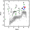 |
Fig. 1. Li abundance as a function of log g. The red square is D25_6334. The blue squares are the three metal-poor stars in E24. Li-rich stars in the literature are shown with black circles (field stars) and green triangles (globular cluster stars), where filled symbols are from L18 and Koch et al. (2011) and open symbols are from the compilation by Mucciarelli et al. (2024). The gray dots are stars with [Fe/H]<−1.3 from the GALAH survey (Buder et al. 2021; Wang et al. 2024). |
E24_1350 and E24_5136 show clear Na enhancement. The NH feature, which we used for N abundance measurement for D25_6334, is not covered in the spectra of these two stars. E24_6328 shows a slight C depletion, slight N enhancement, and subtle Na enhancement compared to typical metal-poor stars, but each of these signatures is subtle and does not represent a significant deviation from typical metal-poor stars. We do not detect any abundance anomalies in other elements for the three stars.
These abundance features of D25_6334 and three E24 stars are consistent with the properties of the six previously identified, unevolved Li-rich stars shown in Fig. 2 (Koch et al. 2011; Pasquini et al. 2014; Li et al. 2018, 2022). D25_6334, E24_1350, and E24_5136 show clear Na enhancement similar to most of the Li-rich stars, while the Na enhancement in E24_6328 is tenuous, which is also seen in a minor fraction of Li-rich stars. There has been no measurement of N abundance for unevolved Li-rich stars in the literature, and hence we cannot conclude if the N enhancement seen in D25_6334 is common among unevolved Li-rich stars.
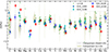 |
Fig. 2. Abundance patterns of D25_6334, the three stars from E24, and Li-rich stars from L18, compared to typical metal-poor stars, which are shown as violin plots. One of the comparison samples is taken from D25, in which abundances were derived consistently with the present study. The other comparison sample was taken from Li et al. (2022), which mostly contains stars with [Fe/H]<−2. Note that Li-rich stars in L18 were reanalyzed by Li et al. (2022), and we used the latter abundance for consistency. Five unevolved Li-rich stars in Li et al. (2018) are shown with filled symbols, and the other more evolved Li-rich stars are shown with open symbols. |
While the three stars from E24 are known to have massive nonluminous companions, other known unevolved Li-rich stars do not necessarily show radial velocity variation (Koch et al. 2012; Li et al. 2018). There is no evidence for the presence of a companion star in the radial velocity measurements of D25_6334. The relative radial velocity between the two UVES observations was estimated to be 0.36 km s−1 by cross-correlating the two spectra. This is likely to be insignificant compared to the systematic uncertainty, which can be up to ∼0.5 km s−1 (Whitmore et al. 2010). Further, we note that the telluric lines in the two spectra are shifted by around 0.5 km s−1. While all the currently available measurements seem to be consistent with each other, future multi-epoch spectroscopy and astrometry that will be available following Gaia DR4 will provide a more robust conclusion on the binarity of D25_6334. For now, we simply note that D25_6334 is similar to the majority of the known unevolved Li-rich stars in the sense that they have not shown radial velocity variation so far (Li et al. 2018; Aoki et al. 2022).
We also note that there is no indication of ongoing stellar activity in the spectrum of D25_6334. Neither emission lines, fast rotation, nor infrared excess are detected for the object.
5. Discussion
The origin of Li-rich stars is still an open question. One of the proposed scenarios is the production of Li in the observed star itself during a certain evolutionary phase near the red clump phase. While this could be the case for the Li-rich stars in the red clump phase (Schwab 2020; Mori et al. 2021; Gao et al. 2022; Denissenkov et al. 2024; Li et al. 2023), it is unlikely for unevolved Li-rich stars, which have not undergone even the first dredge-up. Other scenarios include the engulfment of planets or planetesimal material (e.g., Alexander 1967; Siess & Livio 1999), transfer of Li-rich material from an evolved companion, and Li production inside the star and transport of the produced Li to the surface through merger-induced mixing (Kravtsov et al. 2024).
In this section, we interpret the abundance pattern of D25_6334 and attempt to narrow down the origin of unevolved Li-rich stars, assuming that the enhanced Li and other features of D25_6334 in its abundance pattern are related and that its abundance patterns are representative of unevolved Li-rich stars. Since D25_6334 has one of the largest [Na/Fe] values among the unevolved Li-rich stars, the second assumption may not be valid. However, we stick to this assumption and only discuss D25_6334 in the present study. This is because most other objects do not have N abundance measurements, which plays a crucial role in interpreting the abundance pattern as we see below. The only other object with a N abundance measurement is E24_6328, but it does not exhibit a Na enhancement – a common feature among most Li-rich stars – and hence may not be a good representative of unevolved Li-rich stars.
Since D25_6334 is unevolved, it is relatively safe to assume that the surface chemical composition has not been altered by the evolution of the star itself since its formation or the event that led to the Li enhancements, allowing us to use all the elements, including C and N, to constrain the formation mechanism. We have also shown that at least two of the three metal-poor stars from E24 show abundance patterns similar to D25_6334 and other known unevolved Li-rich stars, suggesting that the formation models need to be able to explain the presence of Li-rich stars without companions and those with massive compact companions.
As is discussed in L18, the planet engulfment scenario is unlikely for metal-poor Li-rich stars, since planets are expected to be rare in metal-poor environments (e.g., Wang & Fischer 2015; Andama et al. 2024). The high [N/Fe] and [Na/Fe] abundances are also difficult to explain by this scenario, since they have lower condensation temperatures than Li (Lodders 2003). The merger-induced nucleosynthesis and mixing also seems unlikely, since the production of C, which requires a high temperature (≳108 K), would be needed to explain the enhanced C + N abundance of [C+N/Fe] = 0.72.
The remaining scenario is the transfer of Li-rich material from (a) companion(s). We discuss here two possibilities: pollution from a giant star and pollution from a classical nova (Fig. 3). Below, the abundance pattern of D25_6334 is compared to the theoretical chemical yields of giant star models and nova models to see if either of these scenarios can explain the observed abundance. We express the predicted abundance pattern as a mixture of material with a typical abundance pattern of metal-poor stars and the theoretical chemical yields of nucleosynthesis in a giant and nova. We define the non-polluted abundance in [X/H] ([X/H]0) using the median [X/Fe] values of all 41 stars in D25 and the metallicity of D25_6334. The theoretical chemical yields in [X/H] ([X/H]model) are obtained from [X/Fe] (Ventura et al. 2013; Cristallo et al. 2015), overproduction factors (Karakas 2010; Doherty et al. 2014), or yields (Ritter et al. 2018) assuming [Fe/H]=−2.1 for giant star models and from the mass fraction of elements in ejecta for nova models (José & Hernanz 1998; José et al. 2020; Starrfield et al. 2020, 2024). We then fit the observed [X/H] of D25_6334 ([X/H]target) by minimizing the following mean squared error:
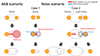 |
Fig. 3. Schematic diagrams of formation scenarios of unevolved Li-rich stars considered in this study. In the AGB scenario shown in the leftmost column, the pollution occurs from a giant star to the currently observed star. The donor star is now expected to be a white dwarf. The remaining columns show scenarios in which pollution from a classical nova is considered. Depending on whether the currently observed star was the donor or not, we further divided the nova scenario into cases 1 and 2. The final state of the nova scenario can be a single, binary, or triple-star system. |
![$$ MSE(\mu ) = \sum _{i} \left ( {\mathrm {[{X}/H]}}_{i,{\rm target}}-\log (\mu 10^{ {\mathrm {[{X}/H]}}_{i, {\rm model}}}+(1-\mu )10^{ {\mathrm {[{X}/H]}}_{i,0}}) \right ) ^2, $$](/articles/aa/full_html/2025/07/aa54264-25/aa54264-25-eq1.gif)
where μ is the dilution factor with 0<μ<1, which is the ratio of the hydrogen mass of an accretion origin (XaccMacc) to the total hydrogen mass after the accretion in the convective envelope of D25_6334 (XenvMenv). We used abundances of C, N, Na, Mg, Al, and Si as these are provided in all the models considered here. Li is not included in this fitting because theoretical prediction tends to be highly uncertain, but we discuss if the observed Li abundance of D25_6334 and those of typical unevolved Li-rich stars can be reproduced by the combination of μ and the expected range of Li production. We also note that s-process elements are not included either, since they are not provided in every model, but we do compare the predicted Sr and Ba abundances with the observation when available.
5.1. Pollution from a giant star
A comparison to AGB star models is of particular interest, since Li production is suggested in AGB stars (Sackmann & Boothroyd 1992). The high C + N abundance also requires the companion to be an AGB star, as C needs to be synthesized through He-burning and some of the produced C needs to be converted to N before the mass transfer event. We thus considered AGB models from Karakas (2010), Ventura et al. (2013), Cristallo et al. (2015, FRUITY), and Ritter et al. (2018, NuGrid) and super AGB models from Doherty et al. (2014) and compared them to the observed abundance pattern of D25_6334. Depending on the availability, we chose models that match the metallicity of D25_6334, [Fe/H]∼−2.1, i.e., Z = 0.0003 for Ventura et al. (2013) and Cristallo et al. (2015) and Z = 0.0001 for Karakas (2010), Ritter et al. (2018), and Doherty et al. (2014). The results of the fitting are shown in Fig. 4 and summarized in Fig. 5.
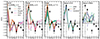 |
Fig. 4. Abundance pattern of D25_6334 (black points) compared to the theoretical chemical yields from AGB stars from Ventura et al. (2013, V13), Cristallo et al. (2015, FRUITY), Karakas (2010, K10), Ritter et al. (2018, NuGrid), and Doherty et al. (2014, D14) and those from nova models from José & Hernanz (1998, JH98), José et al. (2020, J20), Starrfield et al. (2020, S20), and Starrfield et al. (2024, S24). The small gray dots show abundances that a star with the same metallicity as D25_6334 would have if it had [X/Fe] values equal to the median values of all the stars in D25. The yield from each model is diluted with the non-polluted abundance (see text). |
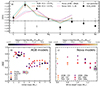 |
Fig. 5. Summary of the comparison between the observed abundance pattern of D25_6334 and the theoretical chemical yields from AGB stars and nova models. Panel a) is the same as Fig. 4 but only for four selected models. Panels b) and c) summarize the square root of the sum of the mean squared error for each model for AGB scenario (b) and for nova scenario (c). The color indicates the dilution factor, defined as the ratio of the hydrogen mass of accretion origin to the total hydrogen mass in the envelope after the accretion (see text). The four models selected in panel a) are highlighted with open circles. They are the 3.0 M⊙ and 3.5 M⊙ AGB models from Ventura et al. (2013), the “ONe6” nova model from José & Hernanz (1998), and the 1.35 M⊙ nova model from Starrfield et al. (2024). |
Although no single model of AGB stars can fit the observed abundance pattern of D25_6334 perfectly, we can still obtain some insights from the comparison. Except for the FRUITY model, high [N/Fe] and [N/C] ratios are realized in intermediate-mass AGB stars with the initial mass of Mini≳3 M⊙ as a result of hot bottom burning. Such models also predict high Na abundances at Mini≲5 M⊙. This may suggest that the most promising companion is an AGB star with Mini∼4 M⊙. Among such intermediate-mass AGB models, 3 M⊙ and 3.5 M⊙ models from Ventura et al. (2013) particularly show good fits to the observed abundance pattern of D25_6334 (Fig. 5). The good match of the observed abundance pattern with the intermediate-mass AGB models is consistent with the scenario proposed by Sayeed et al. (2024) for more metal-rich Li-rich stars at the base of RGB. However, we note that their conclusion is based on slight s-process enhancements, such as in Sr and Ba, in the Li-rich stars, which is not observed in D25_6334. Such intermediate-mass AGB stars are indeed expected to produce some s-process elements, but s-process enhancements might be at most subtle after the dilution (see FRUITY and Nugrid model predictions in Fig. 4).
In the two best-fitting models from Ventura et al. (2013), the accreted mass consists of about 10% of the final convective envelope. Theoretical predictions show that the surface Li abundance of AGB stars can be A(Li)∼4−5 (e.g., Choplin et al. 2024), which is also confirmed by some observations (e.g., Abia & Isern 1997, 2000). The observed Li abundance of most unevolved Li-rich stars (A(Li)∼3) can easily be reproduced with the obtained dilution factor and the expected Li yield from AGB stars.
While the two models from Ventura et al. (2013) might seem promising from the arguments above, the behavior of AGB yields with initial mass is not straightforward and is highly model-dependent, as is seen in Figures 4 and 5. Thus, we cannot robustly conclude that pollution from an intermediate-mass AGB star is the origin of the Li-rich stars. Further refinements and observational constraints on the AGB evolution are highly desired to reduce the uncertainty in the AGB yields and to come to a more robust conclusion.
In the scenario of pollution from an intermediate-mass AGB star, the presence of a white dwarf companion with ∼0.8−0.9 M⊙ is expected (Ventura et al. 2013). D25_6334, however, shows no observational evidence for the presence of a white-dwarf companion. The RUWE in Gaia DR3, which is an indicator of deviation in astrometry from a single star solution and can be diagnostic of the presence of companions (Penoyre et al. 2020; Belokurov et al. 2020; Castro-Ginard et al. 2024), is small, and there is no variation in radial velocity. If it does not currently have a companion, it might have lost the companion through a dynamical interaction with other objects, or it might have been born from a gas cloud that was rich in AGB ejecta. Future epoch astrometry from the Gaia mission and long-term monitoring of radial velocity variation would be needed to put a strong constraint on the presence of a companion. L18 also reported that the majority of unevolved Li-rich stars do not show radial velocity variation, which implies that D25_6334 is not an exception. Moreover, Li-rich stars known to have companions from E24 have companion masses of >1.2 M⊙, which is inconsistent with the companion mass expected for an intermediate-mass AGB star (0.8−0.9 M⊙). Massive super AGB stars that would leave a massive white dwarf companion do not produce enough Na and are unable to explain the observed Na enhancements (Fig. 4). These inconsistencies between the observations and the expectations are a challenge to the AGB pollution scenario, motivating us to consider other scenarios.
5.2. Pollution from a classical nova
Novae are known from both theoretical studies (Arnould & Norgaard 1975; Starrfield et al. 1978, 2020, 2024; Boffin et al. 1993; Hernanz et al. 1996; José & Hernanz 1998; Denissenkov et al. 2014, 2021; José et al. 2020) and observational studies (Tajitsu et al. 2015, 2016; Izzo et al. 2015, 2018; Molaro et al. 2016, 2020, 2022; Selvelli et al. 2018; Arai et al. 2021) to produce Li. We note here that models tend to underestimate Li production by an order of magnitude compared to the observations (see discussions in Kemp et al. 2022; Gao et al. 2024) and we mainly adopt the observationally constrained Li yield in the following discussion. Pollution from a nova has been proposed in the literature as an origin of excess-Li in Li-rich giants, but it does not seem to be the dominant formation channel of Li-rich giants (Gratton & D’Antona 1989; Casey et al. 2019). However, the viability of this nova pollution scenario for unevolved Li-rich stars has only briefly been discussed in L18 and has not been explored in detail. Here, we use abundance ratios of unevolved Li-rich stars, theoretical and observational constraints on the nova nucleosynthesis, and a population synthesis model of novae to study the viability of the nova channel on unevolved Li-rich stars.
In Figures 4 and 5, we show the fitting results of the nova models of José & Hernanz (1998), José et al. (2020), Starrfield et al. (2020), and Starrfield et al. (2024) to the observed abundance pattern of D25_63343. The ONe6 model from José & Hernanz (1998) provides the best match among the nova models considered here with μ∼10−4.2. The model has a white dwarf mass of 1.35 M⊙ and the degree of mixing between the core and the envelope is 50%. The second-best model is also a nova by a massive ONe white dwarf; the 1.35 M⊙ ONe white dwarf model of Starrfield et al. (2024) fits the abundance pattern of D25_6334 with μ∼10−3.9. The match between the observation and these massive ONe white dwarf models is better than most of the AGB models; the exceptions are just the 3 M⊙ and 3.5 M⊙ models from Ventura et al. (2013), where the fit is similarly good. Since the observations of novae suggest A(Li)∼7 (Kemp et al. 2022), the obtained dilution factors would lead to A(Li)∼3, which is in line with the observed Li abundance of D25_6334.
Thus, we consider the nova pollution scenario to be as promising as the AGB pollution scenario in terms of reproducing the abundance pattern. The main differences between the intermediate-mass AGB models and massive ONe white dwarf novae are the insufficient Na production in the former and the insufficient N production in the latter. Both models predict a mild enhancement in Al, which is not observed in D25_6334. We note that the nova models are calculated for solar metallicity, and the nucleosynthesis in novae at low metallicity has not been extensively studied. According to José et al. (2007), N/C and Na/Al ratios increase at lower metallicity, which is promising for reproducing the abundance pattern.
A nova system needs at least one white dwarf that accumulates material from the companion donor star to explode. One can consider two cases for a star to be polluted by nova ejecta and to be Li-rich (see Fig. 3): case 1, in which the polluted star itself is the donor to the white dwarf, and case 2, in which the star is an outer tertiary to a close binary system that underwent nova explosions. Given that the Li-rich stars considered in the present study are unevolved, and hence have small radii and negligible mass-loss rates through winds, case 1 implies a close binary system transferring mass through Roche-lobe overflow. On the other hand, case 2 does not have any constraints on the separation for the occurrence of novae, but introduces dynamical stability constraints and increases the difficulty in accreting nova ejecta due to increased separation from the accreting white dwarf. In both cases, the distance between the nova and the Li-rich star has to be small enough for sufficient pollution to occur.
The total mass of 7Li in the convective envelope of a Li-rich star (Menv(Li)) can be expressed in terms of its current surface Li abundance (A(Li)), the mass of the convective envelope (Menv, typically 10−3 M⊙ for a metal-poor turn-off star (e.g., Richard et al. 2002; Matrozis & Stancliffe 2016), and the mass fraction of hydrogen (X):
Since the initial Li abundance before the pollution is expected to be around the Spite plateau value (A(Li)∼2.2) (e.g., Spite & Spite 1982a, b; Charbonnel & Primas 2005; Wang et al. 2024), about 85% of Menv(Li) needs to be accreted by the star to be Li-rich. The mass of Li produced in a single nova explosion (Mnova(Li)) can be expressed in terms of the ejecta mass (Mej, typically 10−5 M⊙; José & Hernanz 1998) and the Li mass fraction in it (XLi). Given the observed 7Li or 7Be abundance of classical nova of A(7Li)∼7 (see discussions presented in Kemp et al. 2022; Gao et al. 2024) and the typical mass fraction of hydrogen predicted to be X∼0.3 from nova simulations (José & Hernanz 1998), the mass fraction of Li in the ejecta is expected to be around XLi∼2×10⁻⁵. Thus,
Considering the high nova ejecta velocities, we assume a purely geometric accretion scenario based on the radius of the polluted star and its distance to the nova. The fraction of nova ejecta accreted by the polluted star, facc, is

where R★ is the radius of the star, and d is the distance between the nova and the star. Hence, the total amount of Li that is accreted by the star from Nnova nova explosions can be expressed as


or

Note that these two conditions are the same but are expressed in different units for d. For a star to be Li-rich,
must be satisfied.
Based on these estimates, we discuss cases 1 and 2 in the following using the nova population synthesis model of Kemp et al. (2021). Since we expect small d, ∼ a few solar radii for case 1, we compare Eq. (1) and Eq. (5). It is clear that only a few nova explosions are enough to cause the required amount of Li accretion. While this seems very promising, this scenario has some difficulties in explaining the observed properties of Li-rich stars. As was previously discussed, this scenario presents difficulties when confronted with the lack of close binary companions among most unevolved Li-rich stars. The implied very-low-mass end states (<0.5 M⊙) of this channel (Kemp et al. 2021) are also inconsistent with the effective temperatures and surface gravities of the Li-rich stars.
We therefore discarded case 1 and proceeded to assess the possibility of tertiary pollution described in case 2. In this scenario, the separation between the nova and the tertiary has to be wide enough for the system to be dynamically stable and close enough for the tertiary to be sufficiently polluted by the nova ejecta. We considered triple-star systems consisting of an inner binary that is drawn from the population synthesis model of Kemp et al. (2021) and an outer tertiary with a mass of 0.8 M⊙. We estimated the minimum separation between the nova and the tertiary over the period between the first and the last H nova explosion of the inner binary system using the stability criterion of Eggleton & Kiseleva (1995). The largest value of this period is taken as the minimum separation for the tertiary to be on a stable orbit (aouter,min)4. We then discussed if the condition Eq. (7) could be met for the tertiary with the separation of aouter,min.
Since the parameters that span the widest ranges among different systems in Eqs. (1) and (6) are Nnova and d, the latter of which was now set to aouter,min, we show the number of nova explosions (Nnova) and aouter,min in Fig. 6. With all other parameters fixed to the default, the dashed blue line corresponds to the condition in Eq. (7), while the solid line running parallel to it corresponds to Menv = 5Macc(Li). The latter runs through a region where the number of systems is significantly reduced, which allows us to more clearly separate the systems into two groups with the solid line than with the dashed line. Motivated by the clear separation by the solid line and its proximity to the condition Eq. (7), we selected models below this line as promising candidates for achieving sufficient Li accretion from the inner binary to the tertiary. As the parameters such as XLi and Mej still contain large uncertainties, we consider the use of the solid line instead of the dashed line to be a reasonable choice.
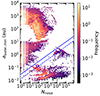 |
Fig. 6. Distribution of nova systems from Kemp et al. (2021) in the space of the minimum separation between the nova and the tertiary (aouter,min) for the stability of the triple-star system and the number of nova explosions (Nnova). The dashed blue line corresponds to the condition Eq. (7), while the solid blue line marks the selection of promising models. The reason for the use of the solid line instead of the dashed line is explained in the text. |
This nova pollution scenario predicts the presence of Li-rich stars without a companion and ones with massive compact companions. The stacked histograms in Figure 7 show the end states of the selected promising binary systems. Interestingly, there is a peak at around the total mass of 1.25 M⊙, which is close to the companion masses of E24_1350 and E24_5136, and the white dwarf mass of the most favored models in the abundance comparisons presented in Fig. 5. There is a tail toward the high mass end among the systems with two remnants, most of which contain two compact objects with a minor contribution from systems comprising one compact object and a normal star. These systems might be an explanation for the companion of E24_6328. It is also promising that some, although not many, nova systems leave no remnants; their tertiary would be observed as a single star like most Li-rich stars.
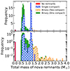 |
Fig. 7. Stacked histogram showing the total mass of remnant systems. The systems are classified by the number of remnants and the number of compact remnants. The upper panel is with the linear scale on the y axis and the lower panel is with the log scale. |
We should, however, note that the nova population synthesis model of Kemp et al. (2021) is based on evolutions in binary systems. Ideally, a dedicated population synthesis model of triple star models is needed for further investigation. First, it needs to be investigated how the outer tertiary can be brought onto an orbit with a sufficiently small separation before the inner binary starts its nova phase. Binary systems going through nova explosions often experience orbital shrinking due to common envelope evolutions. If we were to make a figure similar to Fig. 6 using the minimum separation of a stable triple system at the initial condition of the binary system, almost no models would be selected as promising. Thus, while there are stable orbits for the tertiary to be Li-rich during the nova explosions, the same orbits are not stable when stars are born.
Second, the evolution of triple star systems needs to be followed after the last nova explosion in order to make a comparison with the binary status of the Li-rich stars. The single compact remnant cases in Fig. 7 form through a merger of two objects after the last nova explosion in the system. The system often loses significant mass during this merger process. This raises the question of whether the tertiary can avoid further mass accretion on top of the Li-rich surface and if the tertiary and the remnant can remain bound. This point is a more serious concern for the E24 systems, as their companions are found at the distance of 1−3 au. Due to the mass loss, the separation between the tertiary and the single compact remnant will be widened, and thus it might be difficult to reproduce the binary separation and the mass of the unseen companion of the E24 systems. The modeling of triple-star systems by Shariat et al. (2023, 2025) confirms this finding; the minimum separation possible seems to be in the range of 5−10 au. Future consistent modeling of nova explosions in triple-star systems is desired to conclude if the formation of Li-rich stars with massive compact companions is possible in the nova pollution scenario.
The presence of the tertiary will likely change the evolution of the inner binary system as well. It might reduce the orbital separation of the inner binary, and hence enhance the interaction through the Kozai-Lidov mechanism or dynamical instability, which might lead to a shorter recurrence time of novae (Knigge et al. 2022) and/or the enhanced formation rate of nova systems ending up as type Ia supernova and leaving no remnants (Rajamuthukumar et al. 2023).
5.3. Association with the ED-3 stream
An interesting property of D25_6334 is that it was identified as a member of ED-3. If the progenitor of the stream is a globular cluster, the enhanced N and Na abundances might result from the same formation mechanism as the second-generation stars in globular clusters (see Bastian & Lardo 2018, for a review). However, the metallicity of D25_6334 is significantly lower than the majority of the other stars in the stream, by ∼0.4 dex (D25), indicating that the star does not originate from the same gas cloud as the other stars in the stream if the main progenitor of the stream is a disrupted globular cluster. Since it is still possible that D25_6334 originates from a different globular cluster, future O abundance measurements are of interest to see if the star is a second-generation star from a globular cluster.
If D25_6334 is confirmed to have a globular cluster origin, it will join NGC 6397 #1657 studied by Koch et al. (2011) as an unevolved Li-rich star in globular clusters. The size of such a sample is still small, but it is interesting to see if the formation of unevolved Li-rich stars and multiple populations in globular clusters are related. We note, however, that no globular cluster is known to host a Li-rich population, and thus no clear evidence for the preferred formation of Li-rich stars in globular clusters is known so far. Furthermore, NGC 6397 #1657 does not show N or Na enhancements (Pasquini et al. 2014), features observed in D25_6334. This difference implies that there is likely no relation between the formation of unevolved Li-rich stars and the formation of multiple populations in globular clusters.
An alternative scenario for the formation of the ED-3 stream is that it was a small dwarf galaxy that includes a globular cluster (D25). In this case, it is possible that D25_6334 is a field star in the dwarf galaxy. It is not clear if the formation environment plays a significant role in the formation of unevolved Li-rich stars. In order to investigate this with a larger sample, it is necessary to search for unevolved Li-rich stars among stars that have formed in dwarf galaxies and now in the Milky Way halo, since unevolved stars in surviving dwarf galaxies are out of reach of high-resolution spectroscopy. Such accreted stars can be identified through their kinematics and chemical abundances (e.g., Nissen & Schuster 2010; Helmi et al. 2018)
6. Conclusion
In this paper, we report on the discovery of one new unevolved Li-rich star with a low metallicity ([Fe/H]=−2.1) and the detailed abundance patterns for three similarly Li-rich stars reported in E24. While D25_6334 seems to be a single star, the latter three stars, E24_1350, E24_5136, and E24_6328, are known to each host a relatively massive nonluminous companion. D25_6334 and two of the three stars in E24 show Na enhancements in addition to their Li-excess, a common feature in Li-rich stars. D25_6334 also shows a significant N-excess, and the N abundance of E24_6328 might also be enhanced, but N measurements for the other objects are difficult because of limited wavelength coverage. No noteworthy peculiarities are seen in other elements, including C, Al, and s-process elements, for the four objects. Based on the similarities in the abundance ratios, we suggest that the unevolved Li-rich stars at low metallicity and the metal-poor stars in E24 are in the same class of objects. This would require formation models of unevolved Li-rich stars to reproduce Li-rich stars both with and without close companions.
We also discuss the possible polluters that provided the excess Li, N, and Na to the unevolved Li-rich stars from the abundance pattern of D25_6334, covering C, N, Na, Mg, Al, and Si. The considered polluters include AGB stars modeled by Karakas (2010), Ventura et al. (2013), Cristallo et al. (2015), Ritter et al. (2018), and Doherty et al. (2014) and novae modeled by José & Hernanz (1998), José et al. (2020), Starrfield et al. (2020), and Starrfield et al. (2024). Among the AGB models, two AGB models with 3 and 3.5 M⊙ from Ventura et al. (2013) provide the best matches; however, the results are clearly highly model-dependent, since AGB yields calculated by different groups show a wide variety. In case of pollution from a nova, models involving massive ONe white dwarfs show as good fits as the ones from most AGB models. In either case, further theoretical refinements and observational constraints are needed to make a more robust conclusion; we need more evidence to select the most realistic AGB model, and we need nova models calculated at low metallicity as well as their tests against observations.
While both the AGB and nova scenarios can reproduce the observed abundance pattern of D25_6334, the AGB scenarios predict the presence of a white dwarf companion, which is inconsistent with the observed binary frequency among unevolved Li-rich stars. This inconsistency motivated us to further investigate the nova scenario. We studied the potential configurations that can lead to sufficient mass accretion to the currently observed star in the nova scenario. For unevolved Li-rich stars, the only viable configuration is in triple star systems in which the currently observed star is the outer tertiary to the inner binary that forms a nova system. We selected promising binary configurations that can host a tertiary on a dynamically stable orbit with a small separation and lead to a large number of nova explosions so that sufficient pollution can happen. Interestingly, some such binary systems, although not many, leave no remnants, which is consistent with the observation that a significant fraction of unevolved Li-rich stars do not show any radial velocity variation. They could also leave remnants, a single compact object, binary compact objects, or a binary consisting of a compact object and a star, which could explain the presence of Li-rich stars with massive nonluminous companions, such as those from E24.
The properties of the Li-enhanced binaries discovered by E24 are most readily explained in the nova scenario if the luminous stars are tertiaries orbiting inner binaries containing a massive ONe white dwarf accreting from a low-mass star or brown dwarf. Given the systems’ ancient ages, it is plausible that the accretion rates in the inner binaries would have fallen to sufficiently low levels that no signatures of ongoing accretion are detectable (Knigge et al. 2011). Whether such a scenario can be realized with realistic triple evolution models remains to be seen.
While this paper presents a proof of concept for the nova-pollution scenario, further observational and theoretical studies are needed for a more robust conclusion. First, more intensive radial velocity monitoring is needed to quantify the binary frequency among unevolved Li-rich stars. Second, measurements of detailed abundance patterns, including C, N, O, Na, Mg, and Al, are needed for more objects to obtain better constraints on the polluters. In particular, it is of interest to study if the N enhancements seen in D25_6334 are a common feature among such stars. Theoretically, a population synthesis model of triple star systems is necessary to fully explore the viability of the nova pollution scenario. Population synthesis and nucleosynthesis models also need to be studied at low metallicity.
A measurement of the N isotope ratio provides a robust test for separating the nova and AGB pollution scenarios. Both nova and AGB models can produce enhanced N, but the N isotope ratio is expected to be different between the two sources. If the enhanced N mainly comes from nova, some stars might have a very high 15N abundance, and the isotope ratio 15N/14N could exceed 1 (José & Hernanz 1998). On the other hand, AGB models are not expected to produce a detectable amount of 15N. We thus encourage future attempts to measure the N isotope ratio from analysis of molecular lines in very high-resolution, high-S/N spectra of unevolved Li-rich stars.
Acknowledgments
We thank the anonymous referee for the constructive comments that improved the manuscript. We thank Ko Takahashi and Takuma Suda for the helpful discussions. We also thank Luca Sbordone for his advice on the analysis of the Hα line. TM is supported by a Gliese Fellowship at the Zentrum für Astronomie, University of Heidelberg, Germany. This research was supported in part by Grants-in-Aid for Scientific Research (24K07040) from Japan Society for the Promotion of Science and by a Spinoza Grant from the Dutch Research Council (NWO) awarded to AH.
We note that we re-reduced the raw UVES data to check the blaze function using the UVES data reduction pipeline version 6.4.6 (Ballester et al. 2000).
We used the 25–75% mixing recipe for Starrfield et al. (2020) and Starrfield et al. (2024).
References
- Abia, C., & Isern, J. 1997, MNRAS, 289, L11 [NASA ADS] [CrossRef] [Google Scholar]
- Abia, C., & Isern, J. 2000, ApJ, 536, 438 [NASA ADS] [CrossRef] [Google Scholar]
- Alexander, J. B. 1967, Observatory, 87, 238 [NASA ADS] [Google Scholar]
- Amarsi, A. M., Nordlander, T., Barklem, P. S., et al. 2018, A&A, 615, A139 [NASA ADS] [CrossRef] [EDP Sciences] [Google Scholar]
- Amarsi, A. M., Liljegren, S., & Nissen, P. E. 2022, A&A, 668, A68 [NASA ADS] [CrossRef] [EDP Sciences] [Google Scholar]
- Andama, G., Mah, J., & Bitsch, B. 2024, A&A, 683, A118 [NASA ADS] [CrossRef] [EDP Sciences] [Google Scholar]
- Aoki, W., Li, H., Matsuno, T., et al. 2022, ApJ, 931, 146 [NASA ADS] [CrossRef] [Google Scholar]
- Arai, A., Tajitsu, A., Kawakita, H., & Shinnaka, Y. 2021, ApJ, 916, 44 [Google Scholar]
- Arnould, M., & Norgaard, H. 1975, A&A, 42, 55 [NASA ADS] [Google Scholar]
- Ballester, P., Modigliani, A., Boitquin, O., et al. 2000, Messenger, 101, 31 [NASA ADS] [Google Scholar]
- Bastian, N., & Lardo, C. 2018, ARA&A, 56, 83 [Google Scholar]
- Belokurov, V., Penoyre, Z., Oh, S., et al. 2020, MNRAS, 496, 1922 [Google Scholar]
- Bernstein, R., Shectman, S. A., Gunnels, S. M., Mochnacki, S., & Athey, A. E. 2003, in Instrument Design and Performance for Optical/Infrared Ground-based Telescopes, eds. M. Iye, & A. F. M. Moorwood, SPIE Conf. Ser., 4841, 1694 [NASA ADS] [CrossRef] [Google Scholar]
- Boffin, H. M. J., Paulus, G., Arnould, M., & Mowlavi, N. 1993, A&A, 279, 173 [Google Scholar]
- Buder, S., Sharma, S., Kos, J., et al. 2021, MNRAS, 506, 150 [NASA ADS] [CrossRef] [Google Scholar]
- Cameron, A. G. W., & Fowler, W. A. 1971, ApJ, 164, 111 [NASA ADS] [CrossRef] [Google Scholar]
- Casagrande, L., & VandenBerg, D. A. 2014, MNRAS, 444, 392 [Google Scholar]
- Casey, A. R., Ruchti, G., Masseron, T., et al. 2016, MNRAS, 461, 3336 [NASA ADS] [CrossRef] [Google Scholar]
- Casey, A. R., Ho, A. Y. Q., Ness, M., et al. 2019, ApJ, 880, 125 [Google Scholar]
- Castro-Ginard, A., Penoyre, Z., Casey, A. R., et al. 2024, A&A, 688, A1 [NASA ADS] [CrossRef] [EDP Sciences] [Google Scholar]
- Castro-Tapia, M., Aguilera-Gómez, C., & Chanamé, J. 2024, A&A, 690, A367 [NASA ADS] [CrossRef] [EDP Sciences] [Google Scholar]
- Ceccarelli, E., Massari, D., Mucciarelli, A., et al. 2024, A&A, 684, A37 [NASA ADS] [CrossRef] [EDP Sciences] [Google Scholar]
- Charbonnel, C., & Primas, F. 2005, A&A, 442, 961 [NASA ADS] [CrossRef] [EDP Sciences] [Google Scholar]
- Choplin, A., Siess, L., Goriely, S., & Martinet, S. 2024, Galaxies, 12, 66 [Google Scholar]
- Coc, A., Vangioni-Flam, E., Cassé, M., & Rabiet, M. 2002, Phys. Rev. D, 65, 043510 [Google Scholar]
- Cristallo, S., Straniero, O., Piersanti, L., & Gobrecht, D. 2015, ApJS, 219, 40 [Google Scholar]
- Cyburt, R. H., Fields, B. D., Olive, K. A., & Yeh, T. -H. 2016, Rev. Mod. Phys., 88, 015004 [NASA ADS] [CrossRef] [Google Scholar]
- Deepak, & Lambert, D. L. 2021, MNRAS, 505, 642 [Google Scholar]
- Dekker, H., D’Odorico, S., Kaufer, A., Delabre, B., & Kotzlowski, H. 2000, in Optical and IR Telescope Instrumentation and Detectors, eds. M. Iye, & A. F. Moorwood, SPIE Conf. Ser., 4008, 534 [Google Scholar]
- Deliyannis, C. P., Steinhauer, A., & Jeffries, R. D. 2002, ApJ, 577, L39 [Google Scholar]
- Denissenkov, P. A., Truran, J. W., Pignatari, M., et al. 2014, MNRAS, 442, 2058 [NASA ADS] [CrossRef] [Google Scholar]
- Denissenkov, P. A., Ruiz, C., Upadhyayula, S., & Herwig, F. 2021, MNRAS, 501, L33 [Google Scholar]
- Denissenkov, P. A., Blouin, S., Herwig, F., Stott, J., & Woodward, P. R. 2024, MNRAS, 535, 1243 [NASA ADS] [CrossRef] [Google Scholar]
- Dodd, E., Callingham, T. M., Helmi, A., et al. 2023, A&A, 670, L2 [NASA ADS] [CrossRef] [EDP Sciences] [Google Scholar]
- Dodd, E., Matsuno, T., Helmi, A., et al. 2025, A&A, submitted [2502.17353] [Google Scholar]
- Doherty, C. L., Gil-Pons, P., Lau, H. H. B., et al. 2014, MNRAS, 441, 582 [NASA ADS] [CrossRef] [Google Scholar]
- Eggleton, P., & Kiseleva, L. 1995, ApJ, 455, 640 [NASA ADS] [CrossRef] [Google Scholar]
- El-Badry, K., Rix, H. -W., Latham, D. W., et al. 2024a, Open J. Astrophys., 7, 58 [Google Scholar]
- El-Badry, K., Simon, J. D., Reggiani, H., et al. 2024b, Open J. Astrophys., 7, 27 [NASA ADS] [Google Scholar]
- Fürész, G. 2008, Design and Application of High Resolution and Multiobject Spectrographs: Dynamical Studies of Open Clusters, Ph.D. Thesis, University of Szeged, Hungary [Google Scholar]
- Gao, J., Zhu, C., Yu, J., et al. 2022, A&A, 668, A126 [NASA ADS] [CrossRef] [EDP Sciences] [Google Scholar]
- Gao, J., Zhu, C., Lü, G., et al. 2024, ApJ, 971, 4 [Google Scholar]
- Giribaldi, R. E., da Silva, A. R., Smiljanic, R., & Cornejo Espinoza, D. 2021, A&A, 650, A194 [NASA ADS] [CrossRef] [EDP Sciences] [Google Scholar]
- Gratton, R. G., & D’Antona, F. 1989, A&A, 215, 66 [NASA ADS] [Google Scholar]
- Heiter, U., Jofré, P., Gustafsson, B., et al. 2015, A&A, 582, A49 [NASA ADS] [CrossRef] [EDP Sciences] [Google Scholar]
- Helmi, A., Babusiaux, C., Koppelman, H. H., et al. 2018, Nature, 563, 85 [Google Scholar]
- Hernanz, M., Jose, J., Coc, A., & Isern, J. 1996, ApJ, 465, L27 [NASA ADS] [CrossRef] [Google Scholar]
- Izzo, L., Della Valle, M., Mason, E., et al. 2015, ApJ, 808, L14 [NASA ADS] [CrossRef] [Google Scholar]
- Izzo, L., Molaro, P., Bonifacio, P., et al. 2018, MNRAS, 478, 1601 [NASA ADS] [CrossRef] [Google Scholar]
- Jofré, E., Petrucci, R., García, L., & Gómez, M. 2015a, A&A, 584, L3 [NASA ADS] [CrossRef] [EDP Sciences] [Google Scholar]
- Jofré, P., Heiter, U., Soubiran, C., et al. 2015b, A&A, 582, A81 [Google Scholar]
- José, J., & Hernanz, M. 1998, ApJ, 494, 680 [Google Scholar]
- José, J., García-Berro, E., Hernanz, M., & Gil-Pons, P. 2007, ApJ, 662, L103 [Google Scholar]
- José, J., Shore, S. N., & Casanova, J. 2020, A&A, 634, A5 [EDP Sciences] [Google Scholar]
- Karakas, A. I. 2010, MNRAS, 403, 1413 [NASA ADS] [CrossRef] [Google Scholar]
- Kemp, A. J., Karakas, A. I., Casey, A. R., et al. 2021, MNRAS, 504, 6117 [NASA ADS] [CrossRef] [Google Scholar]
- Kemp, A. J., Karakas, A. I., Casey, A. R., et al. 2022, ApJ, 933, L30 [Google Scholar]
- Knigge, C., Baraffe, I., & Patterson, J. 2011, ApJS, 194, 28 [Google Scholar]
- Knigge, C., Toonen, S., & Boekholt, T. C. N. 2022, MNRAS, 514, 1895 [NASA ADS] [CrossRef] [Google Scholar]
- Koch, A., Lind, K., & Rich, R. M. 2011, ApJ, 738, L29 [NASA ADS] [CrossRef] [Google Scholar]
- Koch, A., Lind, K., Thompson, I. B., & Rich, R. M. 2012, Mem. Soc. Astron. Ital. Suppl., 22, 79 [Google Scholar]
- Kravtsov, V., Dib, S., & Calderón, F. A. 2024, MNRAS, 527, 7005 [Google Scholar]
- Kumar, Y. B., Reddy, B. E., Campbell, S. W., et al. 2020, Nat. Astron., 4, 1059 [NASA ADS] [CrossRef] [Google Scholar]
- Lallement, R., Vergely, J. L., Babusiaux, C., & Cox, N. L. J. 2022, A&A, 661, A147 [NASA ADS] [CrossRef] [EDP Sciences] [Google Scholar]
- Li, H., Aoki, W., Matsuno, T., et al. 2018, ApJ, 852, L31 [NASA ADS] [CrossRef] [Google Scholar]
- Li, H., Aoki, W., Matsuno, T., et al. 2022, ApJ, 931, 147 [NASA ADS] [CrossRef] [Google Scholar]
- Li, X. -F., Shi, J. -R., Li, Y., Yan, H. -L., & Zhang, J. -H. 2023, ApJ, 943, 115 [NASA ADS] [CrossRef] [Google Scholar]
- Lind, K., Nordlander, T., Wehrhahn, A., et al. 2022, A&A, 665, A33 [NASA ADS] [CrossRef] [EDP Sciences] [Google Scholar]
- Lodders, K. 2003, ApJ, 591, 1220 [Google Scholar]
- Mallick, A., Singh, R., & Reddy, B. E. 2023, ApJ, 944, L5 [NASA ADS] [CrossRef] [Google Scholar]
- Martell, S. L., Simpson, J. D., Balasubramaniam, A. G., et al. 2021, MNRAS, 505, 5340 [NASA ADS] [Google Scholar]
- Matrozis, E., & Stancliffe, R. J. 2016, A&A, 592, A29 [NASA ADS] [CrossRef] [EDP Sciences] [Google Scholar]
- Molaro, P., Izzo, L., Mason, E., Bonifacio, P., & Della Valle, M. 2016, MNRAS, 463, L117 [NASA ADS] [CrossRef] [Google Scholar]
- Molaro, P., Izzo, L., Bonifacio, P., et al. 2020, MNRAS, 492, 4975 [NASA ADS] [CrossRef] [Google Scholar]
- Molaro, P., Izzo, L., D’Odorico, V., et al. 2022, MNRAS, 509, 3258 [Google Scholar]
- Monaco, L., Villanova, S., Bonifacio, P., et al. 2012, A&A, 539, A157 [NASA ADS] [CrossRef] [EDP Sciences] [Google Scholar]
- Mori, K., Kusakabe, M., Balantekin, A. B., Kajino, T., & Famiano, M. A. 2021, MNRAS, 503, 2746 [NASA ADS] [CrossRef] [Google Scholar]
- Mucciarelli, A., Bellazzini, M., & Massari, D. 2021, A&A, 653, A90 [NASA ADS] [CrossRef] [EDP Sciences] [Google Scholar]
- Mucciarelli, A., Bonifacio, P., Monaco, L., Salaris, M., & Matteuzzi, M. 2024, A&A, 689, A89 [NASA ADS] [CrossRef] [EDP Sciences] [Google Scholar]
- Nissen, P. E., & Schuster, W. J. 2010, A&A, 511, L10 [NASA ADS] [CrossRef] [EDP Sciences] [Google Scholar]
- Pasquini, L., Koch, A., Smiljanic, R., Bonifacio, P., & Modigliani, A. 2014, A&A, 563, A3 [Google Scholar]
- Penoyre, Z., Belokurov, V., Wyn Evans, N., Everall, A., & Koposov, S. E. 2020, MNRAS, 495, 321 [NASA ADS] [CrossRef] [Google Scholar]
- Rajamuthukumar, A. S., Hamers, A. S., Neunteufel, P., Pakmor, R., & de Mink, S. E. 2023, ApJ, 950, 9 [CrossRef] [Google Scholar]
- Ramírez, I., Meléndez, J., Bean, J., et al. 2014, A&A, 572, A48 [Google Scholar]
- Richard, O., Michaud, G., & Richer, J. 2002, ApJ, 580, 1100 [Google Scholar]
- Ritter, C., Herwig, F., Jones, S., et al. 2018, MNRAS, 480, 538 [NASA ADS] [CrossRef] [Google Scholar]
- Sackmann, I. J., & Boothroyd, A. I. 1992, ApJ, 392, L71 [NASA ADS] [CrossRef] [Google Scholar]
- Sayeed, M., Ness, M. K., Montet, B. T., et al. 2024, ApJ, 964, 42 [NASA ADS] [CrossRef] [Google Scholar]
- Schwab, J. 2020, ApJ, 901, L18 [NASA ADS] [CrossRef] [Google Scholar]
- Selvelli, P., Molaro, P., & Izzo, L. 2018, MNRAS, 481, 2261 [NASA ADS] [CrossRef] [Google Scholar]
- Shariat, C., Naoz, S., Hansen, B. M. S., et al. 2023, ApJ, 955, L14 [Google Scholar]
- Shariat, C., Naoz, S., El-Badry, K., et al. 2025, ApJ, 978, 47 [Google Scholar]
- Siess, L., & Livio, M. 1999, MNRAS, 308, 1133 [Google Scholar]
- Silva Aguirre, V., Ruchti, G. R., Hekker, S., et al. 2014, ApJ, 784, L16 [NASA ADS] [CrossRef] [Google Scholar]
- Singh, R., Reddy, B. E., Bharat Kumar, Y., & Antia, H. M. 2019, ApJ, 878, L21 [NASA ADS] [CrossRef] [Google Scholar]
- Singh, R., Reddy, B. E., Campbell, S. W., Kumar, Y. B., & Vrard, M. 2021, ApJ, 913, L4 [NASA ADS] [CrossRef] [Google Scholar]
- Smiljanic, R., Franciosini, E., Bragaglia, A., et al. 2018, A&A, 617, A4 [NASA ADS] [CrossRef] [EDP Sciences] [Google Scholar]
- Sneden, C. 1973, ApJ, 184, 839 [Google Scholar]
- Spite, M., & Spite, F. 1982a, Nature, 297, 483 [NASA ADS] [CrossRef] [Google Scholar]
- Spite, F., & Spite, M. 1982b, A&A, 115, 357 [NASA ADS] [Google Scholar]
- Starrfield, S., Truran, J. W., Sparks, W. M., & Arnould, M. 1978, ApJ, 222, 600 [NASA ADS] [CrossRef] [Google Scholar]
- Starrfield, S., Bose, M., Iliadis, C., et al. 2020, ApJ, 895, 70 [NASA ADS] [CrossRef] [Google Scholar]
- Starrfield, S., Bose, M., Iliadis, C., et al. 2024, ApJ, 962, 191 [NASA ADS] [CrossRef] [Google Scholar]
- Tajitsu, A., Sadakane, K., Naito, H., Arai, A., & Aoki, W. 2015, Nature, 518, 381 [NASA ADS] [CrossRef] [Google Scholar]
- Tajitsu, A., Sadakane, K., Naito, H., et al. 2016, ApJ, 818, 191 [NASA ADS] [Google Scholar]
- Tayar, J., Carlberg, J. K., Aguilera-Gómez, C., & Sayeed, M. 2023, AJ, 166, 60 [NASA ADS] [CrossRef] [Google Scholar]
- Ventura, P., Di Criscienzo, M., Carini, R., & D’Antona, F. 2013, MNRAS, 431, 3642 [Google Scholar]
- Vogt, S. S., Allen, S. L., Bigelow, B. C., et al. 1994, in Instrumentation in Astronomy VIII, eds. D. L. Crawford, & E. R. Craine, SPIE Conf. Ser., 2198, 362 [Google Scholar]
- Wallerstein, G., & Sneden, C. 1982, ApJ, 255, 577 [NASA ADS] [CrossRef] [Google Scholar]
- Wang, J., & Fischer, D. A. 2015, AJ, 149, 14 [NASA ADS] [CrossRef] [Google Scholar]
- Wang, E. X., Nordlander, T., Asplund, M., et al. 2021, MNRAS, 500, 2159 [Google Scholar]
- Wang, E. X., Nordlander, T., Buder, S., et al. 2024, MNRAS, 528, 5394 [CrossRef] [Google Scholar]
- Whitmore, J. B., Murphy, M. T., & Griest, K. 2010, ApJ, 723, 89 [Google Scholar]
- Yan, H. -L., Zhou, Y. -T., Zhang, X., et al. 2021, Nat. Astron., 5, 86 [NASA ADS] [CrossRef] [Google Scholar]
- Yan, T. S., Shi, J. R., Wang, L., et al. 2022, ApJ, 929, L14 [NASA ADS] [CrossRef] [Google Scholar]
- Zhang, X., Jeffery, C. S., Li, Y., & Bi, S. 2020, ApJ, 889, 33 [NASA ADS] [CrossRef] [Google Scholar]
- Zhou, Y., Wang, C., Yan, H., et al. 2022, ApJ, 931, 136 [NASA ADS] [CrossRef] [Google Scholar]
Appendix A: Spectrum of D25_6334
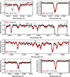 |
Fig. A.1. Portion of the spectrum of D25_6334. The observed spectrum is shown with black dots, and the best-fit synthetic spectra are shown with red lines. The shaded regions show spectra computed with the abundance of the element of ±0.2 dex from the best-fit. The gray lines in the middle two panels show the synthetic spectra with extremely low abundances of C and N, respectively. Note that while spectral fitting was done in LTE, non-LTE correction was applied to Na and Al abundances. |
All Tables
All Figures
|
Fig. 1. Li abundance as a function of log g. The red square is D25_6334. The blue squares are the three metal-poor stars in E24. Li-rich stars in the literature are shown with black circles (field stars) and green triangles (globular cluster stars), where filled symbols are from L18 and Koch et al. (2011) and open symbols are from the compilation by Mucciarelli et al. (2024). The gray dots are stars with [Fe/H]<−1.3 from the GALAH survey (Buder et al. 2021; Wang et al. 2024). |
| In the text | |
|
Fig. 2. Abundance patterns of D25_6334, the three stars from E24, and Li-rich stars from L18, compared to typical metal-poor stars, which are shown as violin plots. One of the comparison samples is taken from D25, in which abundances were derived consistently with the present study. The other comparison sample was taken from Li et al. (2022), which mostly contains stars with [Fe/H]<−2. Note that Li-rich stars in L18 were reanalyzed by Li et al. (2022), and we used the latter abundance for consistency. Five unevolved Li-rich stars in Li et al. (2018) are shown with filled symbols, and the other more evolved Li-rich stars are shown with open symbols. |
| In the text | |
|
Fig. 3. Schematic diagrams of formation scenarios of unevolved Li-rich stars considered in this study. In the AGB scenario shown in the leftmost column, the pollution occurs from a giant star to the currently observed star. The donor star is now expected to be a white dwarf. The remaining columns show scenarios in which pollution from a classical nova is considered. Depending on whether the currently observed star was the donor or not, we further divided the nova scenario into cases 1 and 2. The final state of the nova scenario can be a single, binary, or triple-star system. |
| In the text | |
|
Fig. 4. Abundance pattern of D25_6334 (black points) compared to the theoretical chemical yields from AGB stars from Ventura et al. (2013, V13), Cristallo et al. (2015, FRUITY), Karakas (2010, K10), Ritter et al. (2018, NuGrid), and Doherty et al. (2014, D14) and those from nova models from José & Hernanz (1998, JH98), José et al. (2020, J20), Starrfield et al. (2020, S20), and Starrfield et al. (2024, S24). The small gray dots show abundances that a star with the same metallicity as D25_6334 would have if it had [X/Fe] values equal to the median values of all the stars in D25. The yield from each model is diluted with the non-polluted abundance (see text). |
| In the text | |
|
Fig. 5. Summary of the comparison between the observed abundance pattern of D25_6334 and the theoretical chemical yields from AGB stars and nova models. Panel a) is the same as Fig. 4 but only for four selected models. Panels b) and c) summarize the square root of the sum of the mean squared error for each model for AGB scenario (b) and for nova scenario (c). The color indicates the dilution factor, defined as the ratio of the hydrogen mass of accretion origin to the total hydrogen mass in the envelope after the accretion (see text). The four models selected in panel a) are highlighted with open circles. They are the 3.0 M⊙ and 3.5 M⊙ AGB models from Ventura et al. (2013), the “ONe6” nova model from José & Hernanz (1998), and the 1.35 M⊙ nova model from Starrfield et al. (2024). |
| In the text | |
|
Fig. 6. Distribution of nova systems from Kemp et al. (2021) in the space of the minimum separation between the nova and the tertiary (aouter,min) for the stability of the triple-star system and the number of nova explosions (Nnova). The dashed blue line corresponds to the condition Eq. (7), while the solid blue line marks the selection of promising models. The reason for the use of the solid line instead of the dashed line is explained in the text. |
| In the text | |
|
Fig. 7. Stacked histogram showing the total mass of remnant systems. The systems are classified by the number of remnants and the number of compact remnants. The upper panel is with the linear scale on the y axis and the lower panel is with the log scale. |
| In the text | |
|
Fig. A.1. Portion of the spectrum of D25_6334. The observed spectrum is shown with black dots, and the best-fit synthetic spectra are shown with red lines. The shaded regions show spectra computed with the abundance of the element of ±0.2 dex from the best-fit. The gray lines in the middle two panels show the synthetic spectra with extremely low abundances of C and N, respectively. Note that while spectral fitting was done in LTE, non-LTE correction was applied to Na and Al abundances. |
| In the text | |
Current usage metrics show cumulative count of Article Views (full-text article views including HTML views, PDF and ePub downloads, according to the available data) and Abstracts Views on Vision4Press platform.
Data correspond to usage on the plateform after 2015. The current usage metrics is available 48-96 hours after online publication and is updated daily on week days.
Initial download of the metrics may take a while.