| Issue |
A&A
Volume 699, July 2025
|
|
|---|---|---|
| Article Number | A260 | |
| Number of page(s) | 7 | |
| Section | Planets, planetary systems, and small bodies | |
| DOI | https://doi.org/10.1051/0004-6361/202554197 | |
| Published online | 16 July 2025 | |
No planet around the K giant star 42 Draconis★
1
Thüringer Landessternwarte Tautenburg,
Sternwarte 5,
07778
Tautenburg,
Germany
2
Department of Earth & Planetary Sciences, Weizmann Institute of Science,
Rehovot
76100,
Israel
3
Astronomical Institute, Czech Academy of Sciences,
251 65
Ondrejov,
Czech Republic
4
McDonald Observatory, The University of Texas at Austin,
Austin,
TX
78712,
USA
★★ Corresponding author: This email address is being protected from spambots. You need JavaScript enabled to view it.
Received:
20
February
2025
Accepted:
7
May
2025
Abstract
Context. Published radial-velocity (RV) measurements of the K giant star 42 Dra taken over a three-year time span reveal variations consistent with a 3.9 Jupiter-mass companion in a 479-d orbit.
Aims. This exoplanet can be confirmed if these variations are long-lived and coherent. Continued monitoring may also reveal additional companions.
Methods. We acquired additional RV measurements of 42 Dra; the data now span 15 years. Standard periodogram analyses were used to investigate the stability of the planet’s RV signal. We also investigated variations in the spectral line shapes using the bisector velocity span as well as infrared photometry from the COBE mission.
Results. The recent RV measurements do not follow the published planet orbit. An orbital solution using the 2004–2011 data yields a period and eccentricity consistent with the published values, but the RV amplitude decreased by a factor of four since the earlier measurements. Including some additional RV measurements taken between 2014 and 2018 reveals a second period at 530 d. The interference (beating) of this period with the one at 479 d may account for the observed amplitude variations. The planet hypothesis is conclusively ruled out by COBE/DIRBE 1.25 μ photometry, which shows variations with the planet orbital period as well as a 170 d period.
Conclusions. The RV of 42 Dra shows significant amplitude variations, which along with the COBE/DIRBE photometry firmly established that there is no giant planet around this star. The presence of multi-periodic variations suggests that we are seeing stellar oscillations in this star, most likely oscillatory convection modes. These oscillations may account for some of the long-period RV variations attributed to planets around K giant stars that may skew the statistics of planet occurrence around intermediate-mass stars. Long-term monitoring with excellent sampling is required to exclude amplitude variations in the long periods found in the RV of K giant stars.
Key words: stars: oscillations / planetary systems / stars: individual: 42 Dra / stars: variables: general
Based in part on observations obtained at the 2-m Alfred Jensch Telescope at the Thüringer Landessternwarte Tautenburg.
© The Authors 2025
 Open Access article, published by EDP Sciences, under the terms of the Creative Commons Attribution License (https://creativecommons.org/licenses/by/4.0), which permits unrestricted use, distribution, and reproduction in any medium, provided the original work is properly cited.
This article is published in open access under the Subscribe to Open model. This email address is being protected from spambots. You need JavaScript enabled to view it. to support open access publication.
1 Introduction
Radial velocity (RV) surveys of K giant stars have shown to be effective means of probing planet formation around intermediate-mass (IM) stars of 1.3–2 M⊙. These measurements for IM main-sequence stars are not conducive for RV planet-search surveys, since A to early F stars have high effective temperatures, which results in relatively few spectral lines. These stars also tend to have high rates of rotation. A low number of broad spectral lines results in an RV precision of several tens to hundreds of meters per second making the detection of substellar companions difficult. On the other hand, IM stars that have evolved up the giant branch have cooler effective temperatures, and thus more spectral lines and much slower rotation rates. They are therefore highly amenable to Doppler surveys for planet searches. There have been several studies of planetary companions to K giant stars with the Doppler method (e.g., Frink et al, 2002; Setiawan et al. 2003; Döllinger et al. 2007; Johnson et al. 2007; Sato et al. 2008; Niedzielski et al. 2009; Wittenmyer et al. 2011; Jones et al. 2011; Lee et al. 2012). These surveys have discovered over 100 giant planets around IM evolved stars. However, K giants have their own disadvantages for Doppler surveys. First, these stars have p-mode oscillations that introduce intrinsic variations in the form of RV jitter. The amplitudes are proportional to the luminosity of the star (Kjeldsen & Bedding 1995), so this RV jitter becomes larger as one moves up the giant branch. For stars near the bottom of the giant branch, this is as low as a few meters per second and can be as high as tens of meters per second for a more evolved star. Second, they can exhibit rotational modulation due to stellar structure most likely associated with magnetic activity. The expected rotational periods are several hundreds of days, which is comparable to the orbital periods found for many sub-stellar companions to K giant stars. The first hint for rotational modulation induced RV variations was in α Boo. Hatzes & Cochran (1993) found RV variations with a period of 231 d, nearly identical to the 233 d rotational period inferred from He I 10 830 Å variations by Lambert (1987). Finally, these stars may have new and unknown types of oscillations.
Unfortunately, we know very little about activity and stellar structure on slowly rotating single giant stars, or even the presence of long-period oscillations. To exclude the possibility of rotational modulation as a source of the RV variability, most investigators look for variations in standard activity indicators. These include photometry, often utilizing the archival photometry from the astrometric space mission HIPPARCOS, Ca II H & K, the Ca II infrared triplet, or Hα (e.g., Hatzes et al. 2015). If variations are found in any of these indicators with the same period as the RV variations, serious doubt is cast on the planet hypothesis.
Stellar line bisectors have also become a common tool for proving the planet hypothesis. If any surface inhomogeneities (spots, abundance, convective velocities, etc.) are present, they will likely be accompanied by variable distortions in the spectral line shapes. Indeed, it is these line distortions that mimic an RV variation by causing a shift in the centroid of the spectral line as the star rotates. Line bisector measurements were used to show that the RV variations of HD 166435 were due spots rather than a short-period giant planet (Queloz et al. 2001) as well as to confirm the planet hypothesis for 51 Peg b (Hatzes et al. 1998).
Spectral line bisector variations generally require spectra taken at very high resolving power (R = λ/δλ ≥ 100 000). With data taken at lower spectral resolutions, a lack of bisector variations is a necessary condition to confirm a planet, but it is by no means a sufficient one. A case in point is the purported planet around TW Hya. RV measurements showed evidence of the presence of a short-period Jupiter-mass planet around this T Tauri star (Setiawan et al. 2008). These measurements were taken at reasonably high resolution (resolving power, R = λ/δλ = 45 000). An observed lack of a correlation between the RV and the spectral line bisector variations presumably “confirmed” the planet. However, subsequent RV measurements taken in the infrared showed that these had one-third of the amplitude of the optical measurements (Huélamo et al. 2008). The periodic RV signal was clearly due to spots. So, the generally accepted procedure for confirming the planetary nature of periodic RV signal is to look at as many ancillary data as possible. If one does not see the RV period in any of these, then the planet hypothesis is “confirmed”. However, for giant stars this lack of variability may lead to false conclusions.
In an extensive study of Aldebaran, Hatzes et al. (2015) analyzed 30 years of RV data for this star. These seemed to show a long-lived periodic signal at 629-d that was interpreted as being due to a planetary companion. There were no variations at the 629-d RV period in the equivalent widths of the activity indicators Hα or Ca II λ8662, HIPPARCOS photometry, or in the spectral line shapes. An additional, intermittent signal at 520-d was seen in the RV residuals, Hα and Ca II, and at one-third of this period in the spectral line bisectors. The planet hypothesis was the logical conclusion. However, Reichert et al. (2019) argued against the planet hypothesis based on additional RV measurements. These showed that the ~620-d period had phase shifts, and there were times when it was not present at all.
The K giant star γ Dra also showed evidence of a “fake” planet. Seven years of RV measurements showed coherent, long-lived periodic variations at 702 d consistent with an 11 MJup companion (Hatzes et al. 2018). The lack of variability at this period in the Ca II S-index, spectral line shapes, and HipparCOS photometry seemed to support the planet hypothesis. In fact, the authors were preparing a paper as a planet discovery around γ Dra when more RV measurements spanning an additional two years became available. These showed that the 702-d period disappeared during 2011–2017, only to return in 2014, but with a phase shift. This behaviour was reminiscent of that seen in Aldebaran and thus refuted the planet hypothesis.
At the Thüringer Landessternwarte Tautenburg (TLS), we have been monitoring a sample of K giant stars with the Doppler method to search for exoplanet companions. This program has resulted in discoveries of the planetary companions around 4 UMa (Döllinger et al. 2007), 42 Dra and HD 139357 (Döllinger et al. 2009b; hereafter D09), 11 UMi, and HD 32518 (Döllinger et al. 2009a). RV measurements of the giant star 42 Dra varied with a period 479.1 d and a K-amplitude of K = 110.5 m s−1. This was consistent with the presence of a substellar companion with a minimum mass of 3.9 MJup. HIPPARCOS photometry showed no variations with the RV period. Furthermore, the RV signal seemed to be relatively long-lived and coherent, having the same amplitude for almost three full orbital periods (or about 3.3 years). No bisector measurements were performed on the star, but measurements of the equivalent width of the Hα line showed no correlation with the RV data. The RV variations showed all the earmarks of them stemming from a planetary companion.
We continued to monitor 42 Dra with RV measurements for an additional nine years, three of which had good cadence. This was not only to confirm the planet hypothesis for the 479-d variations (given the experience with Aldebaran and γ Dra), but also to look for additional companions. An examination of the infrared photometry from the COBE mission was also done. All these show that the RV variations seen in 42 Dra do not arise from the orbital reflex motion of the host star due to a substellar companion.
Stellar Parameters for 42 Dra.
2 Stellar parameters
Since stellar parameters for evolved stars are often not included in catalogs such as Gaia (Gaia Collaboration 2021) or the TESS Input Catalog (Paegert et al. 2021), we derived these values using the open-source package Stellar Parameters of Giants and more (Stock et al. 2018). SPOG+ uses Bayesian inference along with observational data to derive fundamental stellar properties, which are listed in Table 1 with the input parameters and their sources. All parameters are very well-constrained, and we found that they are in good agreement with those stated in other papers (e.g., Yu et al. 2023; Khalatyan et al. 2024).
The stellar radius from SPOG+ also agrees well with the radius measured via interferometry. Baines et al. (2018) measured an angular diameter of 2.048 ± 0.009 mas for 42 Dra. Using the Gaia parallax, this results in a stellar radius of R = 19.78 ± 0.17 R⊙.
RV measurements for 42 Dra 2004–2011.
RV measurements for 42 Dra 2014–2018.
3 Data acquisition
From 2008–2011, observations were made with very good cadence using the Tautenburg Coude Echelle Spectrograph (TCES) of the 2-m Alfred Jensch Telescope. The spectral data covered a wavelength region of 4700 Å to 7400 Å at a spectral resolving power of R = 67 000. An iodine absorption cell placed in the optical path was used to provide the wavelength reference for the precise stellar RVs (see Hatzes et al. 2005).
Between 2014 and 2018, additional measurements were made, but with significantly reduced cadence. These were also taken with a different instrumental setup, namely a new echelle grating and a new CCD detector. These data will have a different zero-point offset compared to the 2008–2011 measurements.
Table 2 lists the RV measurements from 2004–2011. These include values derived from previously published data. Since the RV analysis was done on the full data set, values differ from the those published in D09. Table 3 is for the RV measurements from 2014–2018. RVs were produced with the pipeline viper (Zechmeister et al. 2021; Köhler et al. 2025).
Our approach is to first examine the data taken in 2008 − 2011 when the “planet” signal was present to see if these give early hints that it is not a planet. RV measurements in the final years were added to the analysis to shed light on the true nature of the RV variations.
4 Results
Figure 1 shows the RV measurements from 2004–2011 as well as the orbital solution of D09 whose parameters are P = 479.1 ± 6.2 d, e = 0.38 ± 0.06, ω = 218.7 ± 10.6 degrees, and K = 110.5 ± 10.6 m s−1. Clearly, the measurements taken from JD = 2 454 600 to 2 455 600 do not fit the orbit.
We performed an orbital solution using the 2004–2011 data set. The parameters are listed in Table 4. The period and eccentricity agree with the orbital solution of D09, but the full data set yields a slightly shorter period of 474 d. In the discussion that follows we refer to the planet period by its original value of 479 d. Overall, one could still conclude that the signal of the planetary companion was present for at least seven years. However, there is a discrepancy in that the current K-amplitude (65 m s−1) is nearly a factor of two smaller than the earlier K-amplitude of 110 m s−1.
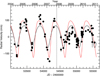 |
Fig. 1 RV measurements for 42 Dra. The vertical dashed line marks the boundary between the old and new RV measurements. The dashed curve is the orbital solution from D09, and the solid curve shows a new solution based on the 2004–2011 data. |
Orbital solution for hypothetical 42 Dra b.
4.1 Amplitude variations
We investigated whether the high cadence data from 2004 − 2011 alone were sufficient to provide strong evidence against the planet hypothesis. The top panel of Figure 2 shows the LombScargle (L-S) periodogram (Scargle 1982) of the data up to JD = 2 454 337. One sees the significant signal at a frequency of ν = 0.0021 d−1, near the orbital frequency that was first reported in D09. On the other hand, the periodogram for the RV data from JD = 2 454 660–2 455 549 shows no significant peak at the planet’s orbital period (central panel). The strongest peak is at ν = 0.00327 d−1 (P = 305 d) and is moderately significant with a false alarm probability (FAP) ≈0.3%.
We checked whether the original 479 d period could have been detected in the RV data JD = 2 454 660–245 549 if it were indeed present. We sampled the original orbital solution shown in Figure 1 in the same manner as the real data and added noise at a level of 55 m s−1. This value is much higher than our typical measurement error, but it is the level of the scatter about the orbital solution. It is also consistent with the level of RV jitter expected from stellar oscillations in this star (see below).
The lower panel of Figure 2 shows the periodogram of the synthetic data, but only using those time stamps from the middle panel. Clearly, we should have easily detected the orbital motion even when using only the new RV measurements.
The RV data show a clear variation in the amplitude of the 479-d signal. We took our revised orbital solution and used the parameters to fit the RV data up to JD = 2 454 530. All parameters were kept fixed, and only the K-amplitude was allowed to vary. This resulted in K = 96.6 ± 6.3 m s−1 (upper panel of Fig. 3). We then fit the RV data taken after JD = 245 660, again allowing only the RV amplitude to vary. We removed two data points in the fit in order to provide a larger time gap between the two subset data. This resulted in K = 27.4 ± 6.1 m s−1 (lower panel of Fig. 3). If the 479-d period was present, its RV amplitude was reduced by about a factor of four from the earlier measurements. This is inconsistent with the orbital reflex motion of the host star due to a companion.
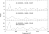 |
Fig. 2 (Top) Lomb–Scargle periodogram of RV measurements up to JD = 2 454 337. (Middle) Periodogram of RV measurements taken after JD ≈ 2 454 660. (Bottom) Periodogram of a simulated orbit over the same time range as the middle panel. The 479-d period should have been present in the periodogram of the latter RV measurements. |
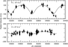 |
Fig. 3 (Top) Orbital solution of the data up to JD ≈ 2 454 400. The K-amplitude is 97 m s−1. (Bottom) Orbital solution to the RV data taken from JD ≈2 454 400–2 455 600. All orbital parameters except the RV amplitude were kept fixed for both data subsets. The K-amplitude for the latter data is 27 m s−1. |
4.2 Frequency analysis of the full data set
We then performed a frequency analysis of the full RV data set covering JD = 2 453 128–2 458 156 (2004–2018), which is shown in Figure 4. This was done using a pre-whitening procedure. Periodic signals were sequentially found and subtracted, and a search for additional signals was carried out on the residuals. The process was stopped when the final peak had a FAP < 0.01. The FAP was estimated from the height of the peak compared to the surrounding noise level. This signal-to-noise ratio (SNR) can be converted into a FAP (Kuschnig et al. 1997; Hatzes 2019). Three significant frequencies were found and are shown in Table 5. The curve in Fig. 4 shows a fit to the RV data using the first two periods (487-d and 530-d), which better demonstrates the interference (beating) between these two dominant periods.
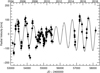 |
Fig. 4 Complete RV measurements of 42 Dra from 2004–2018 (points). The curve represents a two-component fit with two periods: P1 = 487.3 d and P2 = 530 d. |
Frequencies found in full RV data set.
4.3 Examination of the indicators for planet confirmation
As discussed in the introduction, it is wise to look for variations with the RV period in other quantities. If these show variations with the same period as the RV, the planet hypothesis can be rejected. D09 examined the equivalent width of Hα in 42 Dra and found no variations with the RV period, but the authors did not investigate any line shape variations. Here, we take a closer look at the spectral line shapes as well as the HIPPARCOS photometry.
4.3.1 Spectral line shape variations
To investigate changes in the spectral line shapes, we calculated the cross-correlation function (CCF) using the spectral region 4790–4900 Å and the first observation as a template. This region is largely free of the iodine absorption lines that we used for our wavelength calibration. We then calculated the bisector of the CCF – the locus of the midpoints calculated from both sides of the CCF having the same flux value. A linear least-squares fit was then applied to the CCF bisectors. We finally converted this slope between the CCF height values of 0.3–0.85 to an equivalent velocity, which we call the bisector velocity span (BVS).
The top panel of Fig. 5 shows the L-S periodogram of the BVS measurements for 2004–2011 when the planet signal was present. There is a modest peak at a frequency of ν = 0.001497 ± 0.000060 d−1 (P = 671 ± 28 d) with an amplitude of ≈60 m s−1. This frequency is significantly different from the orbital frequency of the purported planet. A bootstrap analysis (see below) indicates a relatively low FAP of ≈5 × 10⁻⁴. The crucial point is that the BVS frequency does not coincide with the orbital frequency.
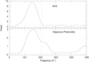 |
Fig. 5 (Top) Lomb-Scargle periodogram of the bisector velocity span (BVS) during the time when the planet signal was present. (Bottom) Lomb–Scargle periodogram of the HIPPARCOS photometry. We note that the photometry was not contemporaneous with the BVS measurements. The dashed vertical line shows the orbital frequency of the purported planet. |
4.3.2 HIPPARCOS photometry revisited
D09 showed that there were no significant variations in the HIPPARCOS photometry with the same period as the RV variations. We took another look at the HIPPARCOS photometry to see if there were any low frequency signals in the data that could coincide with the BVS variations. The lower panel of Fig. 5 shows the low frequency end of the L–S periodogram of the HIPPARCOS photometry. There is indeed a peak at ν = 0.00145 ± 0.00018 d−1 (P = 690 ± 90 d) that is consistent with the one seen in the BVS, but the signal is not very significant (FAP ~ 0.05). The HIPPARCOS photometry does not refute the planet hypothesis.
4.4 DIRBE photometry: final refutation of the planet hypothesis
Price et al. (2010) extracted weekly average near-infrared fluxes for 2652 stars in the all-sky maps of the Diffuse Infrared Background Experiment on the Cosmic Background Explorer (COBE/DIRBE; hereafter DIRBE photometry). We used the time series of 1.25 μm fluxes for 42 Dra to search for periodic signals. Fig. 6 shows the L-S periodogram of the DIRBE photometry. The strongest peak coincides with the orbital frequency of the planet shown by the vertical dashed line. There is a second strong peak at ν = 0.00589 d−1 (P = 169.8 d). Fig. 7 shows the DIRBE photometry phased to the 479-d period.
We assessed the FAP using the boot-strap method (Murdoch et al. 1993). In this method, the RV data are randomly shuffled many (105) times, all while keeping the time stamps fixed. The fraction of random power larger than the data power yields the FAP. Since we are interested in the FAP at a known frequency in the data, we employed a “windowing” bootstrap (Hatzes 2019). The FAP is determined via bootstrap over a modest sized window centered on the frequency of interest. The window was then successively narrowed and a new FAP calculated. The final FAP was the extrapolated value at zero width for the window at the frequency of interest. This resulted in a FAP ≈ 2 × 10⁻³ that random noise could produce the observed power exactly at the planet orbital frequency.
We also assessed the FAP of the second peak using the bootstrap, but over a larger frequency range of ν = 0–0.02 d−1 since the 169.8-d period is not a known signal. After removing the contribution of the 479-d signal, we found a FAP ≈ 0.01; thus, a peak would have higher power anywhere in the frequency range of interest.
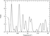 |
Fig. 6 Lomb–Scargle periodogram of DIRBE 1.25 μm photometry. The dashed vertical line shows the orbital frequency of the purported planet. |
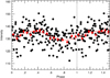 |
Fig. 7 DIRBE photometry phased to the 479-d “orbital” period. The red squares show phase-binned values. The curve represents a sine fit to the data. Data measurements are repeated to the right of the vertical dashed line. |
4.5 Short-term RV variations
As part of our study of 42 Dra we investigated the short-term RV variability by observing the star with high cadence over several nights. Figure 8 shows the best time series from these observations (RV values are listed in Table 6).
A detailed study of the short-term variations is beyond the scope of this work – our observations are too sparse. Nevertheless, we performed a frequency analysis to assess the rough timescales and amplitudes involved. This resulted in two dominant signals, one with frequency ν1 = 0.768 d−1 (P1 = 1.3 d) and RV amplitude K1 = 79.3 m s−1, and one with ν2 = 1.21 d−1 (P = 0.82 d) and RV amplitude K2 = 49.2 m s−1. The curve in the figure shows the two-component fit.
Clearly, these are p-mode oscillations. Kjeldsen & Bedding (1995) gave simple scaling relations for the frequency of maximum power, νmax, and amplitudes for these stellar oscillations. Using the stellar parameters of 42 Dra, these scaling relationships give νmax ≈ 0.88 d−1 (P = 1.14 d), close to our value for ν1. These relationships also give a predicted velocity amplitude of ≈30 m s−1.
Kjeldsen & Bedding (2011) gave revised scaling relations for the oscillation amplitude – taking into account the stellar temperature – with a stronger dependence on the stellar mass. These require a knowledge of the mode lifetimes, which are not well known for an evolved K giant star such as 42 Dra. Assuming a mode lifetime comparable to that of the Sun (≈2.9 days) results in a velocity amplitude of ≈15 m s−1. However, red giant stars can have mode lifetimes of up to a month (De Ridder et al. 2009) or even more for a giant such as 42 Dra. This results in a predicted oscillation amplitude of ≈50 m s−1. Thus, the observed amplitudes for the short-term variations in 42 Dra are entirely consistent with stellar oscillations.
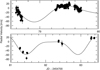 |
Fig. 8 Short-term RV variability of 42 Dra over several nights. The curve is a two-period fit with period, P1 = 1.3 d, amplitude K1 = 79.3 m s−1; P = 0.82 d, K2 = 49.2 m s−1. |
Short-term RV measurements for 42 Dra.
5 Discussion
Precise RV measurements of 42 Dra taken between 2004 and 2008 reveal variations with a period of 479 d and an amplitude of 110 m s−1 that were attributed to a planetary companion (D09). This detection passed all the standard tests for planet confirmation. There were no Hα variations indicative of activity. HIPPARCOS photometry and line bisectors showed variations with a period of 690-d that were well separated from the orbital period of the purported planet. Furthermore, the 479-d variations were coherent and present for at least four years. As a planet detection, 42 Dra b was as solid as many other claimed planets. The original conclusion by D09 seemed reasonable.
Additional RV monitoring of this star tells another story. RV measurements taken between 2008 and 2011 show that the K-amplitude decreased abruptly from about 100 m s−1 to 27 m s−1. Furthermore, if one only considers the RV data from 2008 to 2011, a peak in the periodogram appears at the wrong period. Simulations using the published orbital solution sampled in the same manner as the real data indicate that we should have found the planet signal in the subset data. Even in the 2008–2011 data there were indications that the planet was not real, which was finally confirmed by the DIRBE photometry; this showed significant periodic variations exactly at the orbital period of the planet.
A frequency analysis of the full data set spanning 2004–2018 reveals a possible origin of the amplitude variations. This results in an additional period at 530 d. The beating of these two closely spaced periods can mimic amplitude variations (Fig. 4). It is impossible for these two periods to be planetary companions as this would require giant planets in nearly the same orbit. This system would be dynamically unstable.
It is beyond the scope of this paper to perform a detailed dynamical analysis. However, the stability can be estimated by the Hill radius, rH, given by
![Mathematical equation: $\[r_H \approx a\left(\frac{m}{3 M}\right)^{1 / 3},\]$](/articles/aa/full_html/2025/07/aa54197-25/aa54197-25-eq4.png)
where a and m are the semi-major axis and mass of the smaller body, and M is the mass of the star. A minimum separation of approximately 3.5 RH is widely accepted as the minimum requirement for long-term stability. Using the amplitudes and periods from Table 5, our two hypothetical planets would have masses of approximately 3.2 MJup and 2 MJup and semi-major axes of 1.24 AU and 1.32 AU, respectively. Each planet has a Hill radius rH ≈ 0.1, which is comparable to the minimum separation. This suggests an unstable system.
Gladman (1993) also established the stability of a three-body system based on the Hill criterion. Consider a two-planet system with mass m1 and m2 in orbit around a star of mass M. We can denote the semi-major axis of the outer planet by a = 1 + Δ, where Δ is the fractional separation, If the mass ratios of the two planets with respect to the host star are given by μ1 and μ2, orbits are most likely stable if
![Mathematical equation: $\[\Delta>2.4\left(\mu_1+\mu_2\right)^{1 / 3}.\]$](/articles/aa/full_html/2025/07/aa54197-25/aa54197-25-eq5.png)
For the hypothetical planets of 42 Dra, Δ = 0.08, μ1 = 2.8 × 10⁻³, and μ2 = 1.9 × 10⁻³. In this case, Δ is less than 2.4(μ1 + μ2)1/3 = 0.4, so the system is unstable.
It is not clear what the nature of the 479-d RV period is, the one initially attributed to a companion. One candidate would be rotational modulation by surface features. So far, at least five periods have been identified in 42 Dra: ≈480 d (RV and DIRBE photometry), 535 d (RV), 294 d (RV), 690 d (HIPPARCOS photometry and BVS), and 170 d (DIRBE photometry). These are not harmonics of each other, which is typical for rotational modulation, so only one can be the rotation period. The fact that the 479-d period is also seen in the DIRBE photometry suggests that this may be due to rotational modulation by surface features. However, photometric variations were also seen at 690-d in the HIPPARCOS photometry, albeit with lower significance.
One can estimate the rotational period from the radius and the rotational velocity of the star. Jofre et al. (2015) measured a projected rotational velocity v sin i = 1.76 ± 0.45 km s−1 which yields a maximum rotation period of 554 ± 142 d. This is consistent with either the 479-d period or the 690-d period found in the HIPPARCOS photometry and the BVS. We cannot be certain which of these is the rotation period.
Given the large number of periods that may be present in the RV and photometry of 42 Dra, the simplest explanation is that these arise from stellar oscillations. Long-period RV variations with comparable periods have been found in other evolved stars. For example, Jorissen et al. (2016) found RV variations with a K-amplitude of 540 m s−1 and a period P = 285 d in the carbon-enhanced metal-poor (CEMP) star HE 0017+0055. Since variability with similar periods was found in other CEMP stars, they proposed that the RV variations may be due to envelope oscillations. Oscillatory convective modes were suggested for the long-period RV variations in γ Dra (Hatzes et al. 2018). Additional studies, both observational and theoretical, are needed to confirm the type of oscillations seen in 42 Dra. 42 Dra is yet another case where all the standard tools of planet confirmation of an RV discovery seem to have failed. This only emphasizes that when confirming such long-period RV variations in K giant stars, one needs to look not only at as many ancillary measurements as possible (which may still fail), but also to take measurements spanning more than a decade to search for amplitude variations and closely spaced periods. Long-term monitoring of K giants with planet candidates may be essential in order to confirm the planet hypothesis. Additionally, one can use RV measurements taken at infrared wavelengths to confirm planet detections around K giant stars (Trifonov et al. 2015).
Long-period RV variations attributable to stellar oscillations have been found in several K giant stars. This raises the question of how many planets around evolved stars are false planets. The “fake” planets around evolved IM stars may skew the statistics on the frequency of giant planet formation around more stars more massive than the sun, which could have implications for planet formation theories.
It is worth noting that producing “real” planets also has implications in public outreach. Recently, the International Astronomical Union (IAU) started to assign proper names to exoplanets that have been discovered, many of these with the RV method. The planet around 42 Dra was assigned the name Orbitar1, which will now have to be retracted. This is not the first planet to be refuted, nor will it be the last. Besides K giant stars, this has happened with the “disappearance” of planets around the main-sequence stars GL 581 (Forveille et al. 2011; Robertson et al. 2014) and α Cen B (Hatzes 2013; Rajpaul et al. 2016). The 3.2 M⊕ planet claimed around Barnard’s Star (Ribas et al. 2018) was later shown to be a false positive due to the one-year alias of a stellar activity signal (Lubin et al. 2021).
The effort to broaden the appeal of the exciting field of exoplanet research and of 42 Dra b (Orbitar) shows the public that science is a learning process. Scientists sometimes reach false conclusions when in pursuit of the truth. There will continue to be cases where forms of intrinsic stellar variability (sometimes unknown) can mimic a planet signal. Astronomers and the public should realize that many RV planet discoveries are still candidates that must be confirmed by independent methods. We note that the Gaia mission can provide astrometric observations that could confirm the planetary nature of the long-period RV variations in K giant stars. A naming convention is commendable, but it is more important that the IAU adopt a set of criteria that exoplanet discoveries have to pass before they are declared as bona fide planets. The complex RV variability of K giants only highlights our ignorance regarding stellar phenomena in these stars. Continued studies of these stars are required to determine which variations are companions and which are due to intrinsic stellar variability, and these may require dedicated surveys lasting ten years or more.
Data availability
Full Tables 2, 3 and 6 are available at the CDS via anonymous ftp to cdsarc.cds.unistra.fr (130.79.128.5) or via https://cdsarc.cds.unistra.fr/viz-bin/cat/J/A+A/699/A260
Acknowledgements
This research has made use of the SIMBAD database operated at CDS, Strasbourg, France. APH acknowledges the support of DFG grants HA 3279/5-1 and HA 3279/8-1.
References
- Abdurro’uf, Accetta, K., Aerts, C., et al. 2022, ApJS, 259, 35 [NASA ADS] [CrossRef] [Google Scholar]
- Baines, E. K., Armstrong, J. T., Schmitt, H. R., et al. 2018, AJ, 155, 30 [Google Scholar]
- De Ridder, J., Barban, C., Baudin, F., et al. 2009, Nature, 459, 398 [Google Scholar]
- Döllinger, M. P., Hatzes, A. P., Pasquini, L., et al. 2007, A&A, 472, 649 [NASA ADS] [CrossRef] [EDP Sciences] [Google Scholar]
- Döllinger, M. P., Hatzes, A. P., Pasquini, L., et al. 2009a, A&A, 499, 935 [NASA ADS] [CrossRef] [EDP Sciences] [Google Scholar]
- Döllinger, M. P., Hatzes, A. P., Pasquini, L., et al. 2009b, A&A, 505, 1311 [NASA ADS] [CrossRef] [EDP Sciences] [Google Scholar]
- Forveille, T., Bonfils, X., Delfosse, X., et al. 2011, arXiv e-prints [arXiv:1109.2505] [Google Scholar]
- Frink, S., Mitchell, D. S., Quirrenbach, A., et al. 2002, ApJ, 576, 478 [Google Scholar]
- Gaia Collaboration (Brown, A. G. A., et al.) 2021, A&A, 649, A1 [NASA ADS] [CrossRef] [EDP Sciences] [Google Scholar]
- Gladman, B. 1993, Icarus, 106, 247 [Google Scholar]
- Gontcharov, G.A., Mosenkov, A.V. 2017, MNRAS, 472, 3805 [NASA ADS] [CrossRef] [Google Scholar]
- Hatzes, A. P. 2013, ApJ, 770, 133 [NASA ADS] [CrossRef] [Google Scholar]
- Hatzes, A.P., & Cochran, W. D. 1993, ApJ, 413, 339 [CrossRef] [Google Scholar]
- Hatzes, A. P., Cochran, W. D., & Bakker, E.J. 1998, ApJ, 408, 380 [Google Scholar]
- Hatzes, A. P., Guenther, E. W., Endl, M., et al. 2005, A&A 437, 743 [NASA ADS] [CrossRef] [EDP Sciences] [Google Scholar]
- Hatzes, A. P., Cochran, W. D., Endl, M., et al. 2015, A&A, 580, A31 [NASA ADS] [CrossRef] [EDP Sciences] [Google Scholar]
- Hatzes, A.P., Cochran, W. D., Endl, M., et al. 2018, AJ, 155, 120 [NASA ADS] [CrossRef] [Google Scholar]
- Hatzes, A. P. 2019, The Doppler Method for the Detection of Exoplanets, ed. A. P. Hatzes, IOP ebooks (Bristol, UK: IOP Publishing) [Google Scholar]
- Høg, E., Fabricius, C., Makarov, V. V., et al. 2000, A&A, 355, 27 [Google Scholar]
- Huélamo, N., Figueira, P., Bonfils, X., et al. 2008, A&A, 489, 9 [Google Scholar]
- Jofre, E., Petrucci, R., Saffe, C., et al. 2015, A&A, 574, A50 [Google Scholar]
- Johnson, J. A., Fischer, D. A., Marcy, G. W., et al. 2007, ApJ, 665, 785 [Google Scholar]
- Jones, M. I., Jenkins, J. S., Rojo, P., & Melo, C. H. F. 2011, A&A, 536, A71 [NASA ADS] [CrossRef] [EDP Sciences] [Google Scholar]
- Jorissen, A., Van Eck, S., Van Winckel, H., et al. 2016, A&A, 586, A158 [NASA ADS] [CrossRef] [EDP Sciences] [Google Scholar]
- Khalatyan, A., Anders, F., Chiappini, C., et al. 2024, A&A, 691, A98 [NASA ADS] [CrossRef] [EDP Sciences] [Google Scholar]
- Kjeldsen, H., & Bedding, T. R. 1995, A&A, 87, 106 [Google Scholar]
- Kjeldsen, H., & Bedding, T. R. 2011, A&A, 529, L8 [NASA ADS] [CrossRef] [EDP Sciences] [Google Scholar]
- Köhler, J., Zechmeister, M., Hatzes, A., et al. 2025, A&A, 698, A44 [NASA ADS] [CrossRef] [EDP Sciences] [Google Scholar]
- Kuschnig, R., Weiss, W. W., Gruber, R., et al. 1997, A&A, 328, 544 [Google Scholar]
- Lambert, D. L. 1987, ApJS, 65, 255 [NASA ADS] [CrossRef] [Google Scholar]
- Lee, B.-C., Mkrtichian. D. E., Han, I., Park, M.-G., & Kim, K.-M. 2012, A&A, 548, A118 [NASA ADS] [CrossRef] [EDP Sciences] [Google Scholar]
- Lubin, J., Robertson, P., Stefansson, G., et al. 2021, AJ, 162, 61 [NASA ADS] [CrossRef] [Google Scholar]
- Murdoch, K. A., Hearnshaw, J. B., & Clark, M. 1993, ApJ, 413, 349 [CrossRef] [Google Scholar]
- Niedzielski, A., Goździewski, Wolszczan, A., et al. 2009 ApJ, 693276 [Google Scholar]
- Paegert, M., Stassun, K. G., Collins, K. A., et al. 2021, arXiv e-prints [arXiv:2108.04778] [Google Scholar]
- Price, S. D., Smith, B. J., Kuchar, T. A., et al. 2010, ApJ Supp., 190, 203 [Google Scholar]
- Queloz, D., Henry, G. W., Sivan, J. P., et al. 2001, A&A, 379, 279 [NASA ADS] [CrossRef] [EDP Sciences] [Google Scholar]
- Rajpaul, V., Aigrain, S., & Roberts, S. 2016, MNRAS, 456, 6 [Google Scholar]
- Reichert, K., Reffert, S., Stock, S., et al. 2019, A&A, 625, A22 [NASA ADS] [CrossRef] [EDP Sciences] [Google Scholar]
- Ribas, I., Tuomi, M., Reiners, A., et al. 2018, Nature, 563, 365 [Google Scholar]
- Robertson, P., Mahadevan, S., Endl, M., & Roy, A. 2014, Science, 345, 440 [Google Scholar]
- Sato, B., Izumiura, H., Toyota, E., et al. 2008, PASJ, 60, 539 [NASA ADS] [Google Scholar]
- Scargle, J. D. 1982, ApJ, 263, 835 [Google Scholar]
- Setiawan, J., Hatzes, A. P., von der Lühe, O., et al. 2003, A&A, 398, 19 [Google Scholar]
- Setiawan, J., Henning, Th., Launhardt, R., et al. 2008 Nature, 451, 385 [Google Scholar]
- Stock, S., Reffert, S., & Quirrenbach, A. 2018, A&A, 616, A33 [NASA ADS] [CrossRef] [EDP Sciences] [Google Scholar]
- Trifonov, T., Reffert, S., Zechmeister, M., et al. 2015, A&A, 582, A54 [NASA ADS] [CrossRef] [EDP Sciences] [Google Scholar]
- Wittenmyer, R. A., Endl, M., Wang, L., et al. 2001, ApJ, 743, 184 [Google Scholar]
- Yu, J., Khanna, S., Themessl, N., et al. 2023, ApJS, 264, 41 [NASA ADS] [CrossRef] [Google Scholar]
- Zechmeister, M., Köhler, J., & Chamarthi, S. 2021, Astrophysics Source Code Library [record ascl:2108.006] [Google Scholar]
All Tables
All Figures
|
Fig. 1 RV measurements for 42 Dra. The vertical dashed line marks the boundary between the old and new RV measurements. The dashed curve is the orbital solution from D09, and the solid curve shows a new solution based on the 2004–2011 data. |
| In the text | |
|
Fig. 2 (Top) Lomb–Scargle periodogram of RV measurements up to JD = 2 454 337. (Middle) Periodogram of RV measurements taken after JD ≈ 2 454 660. (Bottom) Periodogram of a simulated orbit over the same time range as the middle panel. The 479-d period should have been present in the periodogram of the latter RV measurements. |
| In the text | |
|
Fig. 3 (Top) Orbital solution of the data up to JD ≈ 2 454 400. The K-amplitude is 97 m s−1. (Bottom) Orbital solution to the RV data taken from JD ≈2 454 400–2 455 600. All orbital parameters except the RV amplitude were kept fixed for both data subsets. The K-amplitude for the latter data is 27 m s−1. |
| In the text | |
|
Fig. 4 Complete RV measurements of 42 Dra from 2004–2018 (points). The curve represents a two-component fit with two periods: P1 = 487.3 d and P2 = 530 d. |
| In the text | |
|
Fig. 5 (Top) Lomb-Scargle periodogram of the bisector velocity span (BVS) during the time when the planet signal was present. (Bottom) Lomb–Scargle periodogram of the HIPPARCOS photometry. We note that the photometry was not contemporaneous with the BVS measurements. The dashed vertical line shows the orbital frequency of the purported planet. |
| In the text | |
|
Fig. 6 Lomb–Scargle periodogram of DIRBE 1.25 μm photometry. The dashed vertical line shows the orbital frequency of the purported planet. |
| In the text | |
|
Fig. 7 DIRBE photometry phased to the 479-d “orbital” period. The red squares show phase-binned values. The curve represents a sine fit to the data. Data measurements are repeated to the right of the vertical dashed line. |
| In the text | |
|
Fig. 8 Short-term RV variability of 42 Dra over several nights. The curve is a two-period fit with period, P1 = 1.3 d, amplitude K1 = 79.3 m s−1; P = 0.82 d, K2 = 49.2 m s−1. |
| In the text | |
Current usage metrics show cumulative count of Article Views (full-text article views including HTML views, PDF and ePub downloads, according to the available data) and Abstracts Views on Vision4Press platform.
Data correspond to usage on the plateform after 2015. The current usage metrics is available 48-96 hours after online publication and is updated daily on week days.
Initial download of the metrics may take a while.