© The Authors 2025

1. Introduction

Light nuclear clusters such as hydrogen or helium isotopes are expected to be produced in hot and dense stellar matter, and their abundance is known to affect the dynamical properties of core-collapse supernovae (Arcones et al. 2008; Sumiyoshi & Roepke 2008; Furusawa et al. 2013, 2017; Fischer et al. 2014, 2020) and binary neutron star (NS) mergers (Bauswein et al. 2013; Rosswog 2015; Radice et al. 2018; Psaltis et al. 2024). Even if the weak rates directly involving light clusters are low (Fischer et al. 2020), their abundance is in competition with that of heavy nuclei (Pais et al. 2019), which indirectly affects the neutrino dynamics, and the size and proton fraction of nucleosynthesis seeds (Nedora et al. 2021).

The possible relevance of light clusters in NS physics is much less addressed in the literature. In this paper we explore the possibility that such light composites play the role of impurities in the crustal lattice. Formed from core-collapse supernova explosions, NSs are born hot, with temperatures exceeding several 10¹⁰ K (Haensel et al. 2007). In these conditions, the crust of the proto-NS is a liquid plasma composed of different nuclear species, including light clusters in a background of electrons and nucleons. It is generally assumed that, as the NS crust cools, this multicomponent plasma remains in full thermodynamic equilibrium until the crust crystallizes, and that the composition at the crystallization temperature coincides with the ground-state composition, namely a sequence of pure layers, each consisting of a one-component ideal Coulomb crystal. In this situation, the only nuclear species relevant for the description of a NS are heavy ions with atomic numbers on the order of Z≈20−40.

However, the crustal lattice is not expected to be strictly perfect and can present different defects that are collectively known as impurities. They are quantified via an “impurity parameter” that measures the importance of charge fluctuations at each depth of the crust. In magneto-thermal simulations of NS evolution, this (possibly density-dependent) impurity parameter is typically calibrated on observational cooling data (Viganò et al. 2013). A high impurity parameter value lowers the electrical and thermal conductivity and seems to be needed for a better description of different astrophysical observations concerning isolated X-ray pulsars and late-time cooling in binaries (Pons et al. 2013; Newton 2013; Deibel et al. 2017; Hambaryan et al. 2017; Tan et al. 2018).

If the presence of highly resistive layers due to the existence of impurities seems well established, its physical origin and the actual value of the impurity parameter are less clear. Classical molecular dynamics simulations suggest that the innermost part of the inner crust is composed of disordered and amorphous nuclear matter, with the coexistence of different exotic complex shapes (Schneider et al. 2014; Horowitz et al. 2015; Caplan et al. 2021; Newton et al. 2022). The onset of this pasta mantle is, however, model-dependent (Dinh Thi et al. 2021; Shchechilin et al. 2023), and the most extended part of the inner crust is believed to be composed of standard spherical nuclei (Shchechilin et al. 2024). In the spherical regime it has been suggested that if the one-component plasma approximation is released, different ion species might persist as impurities in the whole catalyzed crust due to the non-adiabaticity of the cooling dynamics (Goriely et al. 2011; Fantina et al. 2020; Carreau et al. 2020; Potekhin & Chabrier 2021; Dinh Thi et al. 2023a). Fantina et al. (2020) and Dinh Thi et al. (2023a) computed the impurity factor self-consistently within a multicomponent approach at different temperatures close to the crystallization temperature. The latter work finds that high impurity parameter values, between Q_imp≈5 and Q_imp≈100, can be obtained in the inner crust, even in the density region where deformed pasta structures are not expected, due to the simultaneous presence at finite temperatures of very neutron-rich light isotopes (Z≈2−3, A≳10) and heavy (Z≈20−30, A≳100) ions. In that study, a single energy functional was employed, and the cluster free energy was computed with the compressible liquid drop (CLD) model, which provides a poor description of the lightest nuclei. Moreover, Dinh Thi et al. (2023a) reached no strong conclusions regarding the possible impact of “non-exotic” composite particles such as α, deuterons, or tritons on the impurity parameter, Q_imp. It is therefore interesting to explore a more accurate and microscopic description of these light-cluster free energies in a dense nuclear medium, and to study possible model dependences. To consider such strongly bound light particles together with heavy nuclei, one has to go beyond the density functional treatment in the Wigner-Seitz approximation and explicitly include them as independent (point-like) quasi-particles, as is done in this work.

From the studies of Fantina et al. (2020) and Dinh Thi et al. (2023a) we expect that important charge fluctuations can only occur if the charge distribution has a multimode structure, with clusters of very different sizes appearing with comparable probability. We therefore considered a simplified theoretical setting in which the one-component plasma approximation is kept for the dominant ion species, but hydrogen and helium isotopes are added, as proposed in previous works (Avancini et al. 2012; Ferreira & Providencia 2012). In the present work, both heavy and light clusters, which were first introduced in Pais et al. (2019), are included within a relativistic mean-field (RMF) formalism; the heavy cluster is described by a CLD model, and the H and He isotopes are taken as new explicit degrees of freedom of the system. The advantage of this description is that in-medium modifications of light-cluster energies in the medium are easily introduced as a modification of the couplings of nucleons bound in clusters with effective mesonic fields (Pais et al. 2018). This effective coupling modification was extensively calibrated on ab initio calculations (Röpke 2015, 2020; Ren et al. 2024) and experimental constraints (Qin et al. 2012; Bougault et al. 2020), in particular for the FSU functional (Pais et al. 2020; Custódio et al. 2020, 2024). Within this formalism, fluctuations of the dominant ion species in the different Wigner-Seitz cells are neglected, as is the possible presence of exotic neutron-rich clusters (Pais et al. 2019). The resulting Q_imp values therefore represent a lower limit to the crustal impurities. Nevertheless, this approach allows us to address the importance of the possible contribution of non-exotic composite particles and their impact on the impurity parameter, independently from the effect of the nuclear distribution discussed in Dinh Thi et al. (2023a).

The paper is organized as follows: In Sect. 2 we introduce the formalism used in this work; in Sect. 2.1 we describe the treatment of homogeneous matter, in Sect. 2.2 that of the (heavier) clusters through the CLD model, and in Sect. 2.3 the treatment of light clusters. We present our numerical results in Sect. 3, and we draw our conclusions in Sect. 4. In this work we consider natural units, where ℏ=c=k_B = 1.

2. Formalism

Each layer of the NS inner crust is described as a collection of identical neutral cells constituted of a single spherical nucleus, and a uniform distribution of dripped neutrons and point-like light clusters, all interacting with and through effective meson fields. The nucleus is treated as a CLD with bulk, surface, and Coulomb terms, in the same spirit as in Pais et al. (2015). Since we studied the liquid phase of the crust, translational degrees of freedom are also associated with the nuclear droplet.

In the following subsections we describe in further detail the theoretical treatment of homogeneous matter (Sect. 2.1), which is used for the bulk part of the droplet energy as well as for the dripped neutrons, the finite-size and translational terms associated with the nuclear droplet within a CLD model (Sect. 2.2), and the treatment of the light clusters (Sect. 2.3).

2.1. Homogeneous matter

Our formalism is based on the nonlinear (NL) Walecka model in the mean-field approximation (Furnstahl et al. 1996, 1997). Within this approach, we considered a homogeneous infinite system of nucleons with mass M (protons p and neutrons n) interacting with and through three meson fields: an isoscalar-scalar field (ϕ) with mass m_s, an isoscalar-vector field (V^μ) with mass m_v and an isovector-vector field (b^μ) with mass m_ρ, for the isospin dependence. Protons and electrons interact through the electromagnetic field A^μ. The Lagrangian density is given as

$$\mathcal{L}={\displaystyle \sum _{j=p,n}}{\mathcal{L}}_j+{\mathcal{L}}_e+{\mathcal{L}}_{\sigma }+{\mathcal{L}}_{\omega }+{\mathcal{L}}_{\rho }+{\mathcal{L}}_{\omega \rho }+{\mathcal{L}}_{\gamma }.$$(1)

The nucleon and electron terms read, respectively,

$${\mathcal{L}}_j={\overline{\psi }}_j\left[{\gamma }_{\mu }{\mathit{iD}}^{\mu }-M^{*}\right]{\psi }_j,$$(2)

$${\mathit{iD}}^{\mu }=i{\partial }^{\mu }-g_v{V}^{\mu }-\frac{g_{\rho }}{2}\tau ·b^{\mu }-e\frac{1+{\tau }_3}{2}{A}^{\mu },$$(3)

$${\mathcal{L}}_e={\overline{\psi }}_e\left[{\gamma }_{\mu }\left(i{\partial }^{\mu }+e{A}^{\mu }\right)-m_e\right]{\psi }_e,$$(4)

and the nucleon Dirac effective mass is given by

$$M^{*}=M-g_s\varphi .$$(5)

The meson and electromagnetic field Lagrangian densities are given by

$${\mathcal{L}}_{\sigma }=\frac{1}{2}\left({\partial }_{\mu }\varphi {\partial }^{\mu }\varphi -m_s^2{\varphi }^2-\frac{1}{3}\kappa {\varphi }^3-\frac{1}{12}\lambda {\varphi }^4\right),$$(6)

$${\mathcal{L}}_{\omega }=-\frac{1}{4}{\mathrm{\Omega }}_{\mu \nu }{\mathrm{\Omega }}^{\mu \nu }+\frac{1}{2}{m}_v^2{V}_{\mu }{V}^{\mu }+\frac{1}{4!}\xi g_v^4(V_{\mu }{V}^{\mu }{)}^2,$$(7)

$${\mathcal{L}}_{\rho }=-\frac{1}{4}{\text{B}}_{\mu \nu }·{\text{B}}^{\mu \nu }+\frac{1}{2}{m}_{\rho }^2{b}_{\mu }·b^{\mu },$$(8)

$${\mathcal{L}}_{\gamma }=-\frac{1}{4}{F}_{\mu \nu }{F}^{\mu \nu },$$(9)

$${\mathcal{L}}_{\omega \rho }={\mathrm{\Lambda }}_v{g}_v^2{g}_{\rho }^2{\text{b}}_{\mu }·{\text{b}}^{\mu }{V}_{\mu }{V}^{\mu },$$(10)

where Ω_μν=∂_μV_ν−∂_νV_μ, B_μν=∂_μb_ν−∂_νb_μ−g_ρ(b_μ×b_ν), and F_μν=∂_μA_ν−∂_νA_μ. The NL ℒ_ωρ term affects the density dependence of the symmetry energy. The models comprise the following parameters: three coupling constants of the mesons to the nucleons, g_s, g_v, and g_ρ, the mixing ωρ coupling, Λ_v, the bare nucleon mass M, the electron mass m_e, the masses of the mesons, the electromagnetic coupling constant $e=\sqrt{4\pi /137}$, and the self-interacting coupling constants κ, λ, and ξ. In this Lagrangian density, τ are the Pauli matrices.

Concerning the choice of the nuclear interactions, we used two families of models: NL models – namely FSU (Todd-Rutel & Piekarewicz 2005), FSU2R (Negreiros et al. 2018), NL3ωρ (Horowitz & Piekarewicz 2001; Pais & Providência 2016), and NLset21 (Malik et al. 2024) – and density-dependent (DD) models – namely TW (Typel & Wolter 1999), DD2 (Typel et al. 2010), and DDME2 (Lalazissis et al. 2005). For NL models, the couplings of the mesons to the nucleons are fixed, and the meson terms included in the Lagrangian density are up to quartic order, as defined above. For DD models, the couplings of the mesons to the nucleons vary with the density. In this case, the self-interaction couplings, κ,λ, and the mixing ωρ coupling, Λ_v, are zero, and the g_s, g_v, and g_ρ couplings are given by the DD functions (Typel & Wolter 1999; Typel et al. 2010; Lalazissis et al. 2005)

$$g_i=g_{i_0}{f}_i(x),i=s,v,$$(11)

$$f_i(x)=a_i\frac{1+b_i(x+d_i{)}^2}{1+c_i(x+d_i{)}^2},$$(12)

$$g_{\rho }=g_{{\rho }_0}exp(-a_{\rho }(x-1)),$$(13)

with x=ρ/ρ₀. The reader can refer to Typel & Wolter (1999), Typel et al. (2010), and Lalazissis et al. (2005) for the values of the parameters a_i,b_i,c_i,d_i for each DD model. DDME2 was fitted to reproduce the properties of symmetric and asymmetric matter, binding energies, and neutron and charge radii of stable nuclei. Moreover, this model is able to reproduce two-solar-mass NSs. DD2 also reproduces properties of finite nuclei and is based on the TW model, the first DD model that appeared in the literature. FSU, on the other hand, is not able to produce two-solar-mass NSs, but it describes the properties of nuclear matter well at and below saturation density (Grill et al. 2014), which is the range of densities considered in this work. However, FSU2R was constructed in order to correct the two-solar-mass problem, and differs from FSU in the isovector sector. NLset21 is a recent model chosen from a set of NL models constructed using Bayesian techniques (Malik & Providência 2022) that fulfill astrophysical, chiral effective-field-theory (EFT) neutron-matter calculations, and also closely reproduce the symmetric matter properties at saturation. NL3ωρ is a model from the NL3 family; it has the same isoscalar properties as NL3, but differs in the isovector properties. Since NL3 has a very large slope of the symmetry energy, L_sym,0 = 118 MeV, the NL3ωρ model is constructed by adding a term mixing ω and ρ mesons in order to lower the value of L_sym,0: the mixing term is varied and the corresponding isovector coupling is calculated so that the symmetry energy at ρ = 0.1 fm⁻³ has the same value as in NL3.

The equilibrium state of asymmetric nuclear matter is characterized by the distribution functions, f_0k±, of particles (+) and antiparticles (−) k=p,n,e, given by

$$f_{0j\pm }=\frac{1}{1+e^{({ϵ}_{0j}\mp {\nu }_j)/T}},j=p,n$$(14)

with

$${ϵ}_{0j}=\sqrt{p^2+{M^{*}}^2},{\nu }_j={\mu }_j-g_v{V}_0^{(0)}-\frac{g_{\rho }}{2}{\tau }_j{b}_0^{(0)},$$(15)

and

$$f_{0e\pm }=\frac{1}{1+e^{({ϵ}_{0e}\mp {\mu }_e)/T}},$$(16)

$${ϵ}_{0e}=\sqrt{p^2+m_e^2},$$(17)

where μ_k is the chemical potential of particle k=p,n,e. The net particle number densities are readily calculated from the distribution functions as

$${\rho }_j=\frac{1}{{\pi }^2}{\displaystyle \int }\mathit{dp}{p}^2\left(f_{0j+}+f_{0j-}\right).$$(18)

In the mean-field approximation, the thermodynamic quantities of interest are given in terms of the meson fields, which are replaced by their constant expectation values (denoted by a subscript “0”).

For homogeneous neutral nuclear matter, the energy density, the entropy density, the free energy density, and the pressure are given, respectively, by

$$\begin{array}{cc}\hfill \mathcal{E}& =\frac{1}{{\pi }^2}\sum _{j=p,n}{\displaystyle \int }\mathit{dp}{p}^2{ϵ}_{0j}\left(f_{0j+}+f_{0j-}\right)\hfill \\ \hfill & +\frac{m_v^2}{2}{V}_0^2+\frac{\xi g_v^4}{8}{V}_0^4+\frac{m_{\rho }^2}{2}{b}_0^2+\frac{m_s^2}{2}{\varphi }_0^2\hfill \\ \hfill & +\frac{k}{6}{\varphi }_0^3+\frac{\lambda }{24}{\varphi }_0^4+3{\mathrm{\Lambda }}_v{g}_{\rho }^2{g}_v^2{V}_0^2{b}_0^2,\hfill \end{array}$$(19)

$$\begin{array}{cc}\hfill \mathcal{S}& =-\frac{1}{{\pi }^2}\sum _{j=p,n}\int \mathit{dp}{p}^2[f_{0j+}ln{f}_{0j+}\hfill \\ \hfill & +(1-f_{0j+})ln(1-f_{0j+})+f_{0j-}ln{f}_{0j-}\hfill \\ \hfill & +(1-f_{0j-})ln(1-f_{0j-})],\hfill \end{array}$$(20)

$$\mathcal{F}=\mathcal{E}-\mathit{TS},$$(21)

$$\begin{array}{cc}\hfill P& =\frac{1}{3{\pi }^2}\sum _{j=p,n}\int \mathit{dp}\frac{p^4}{{ϵ}_{0j}}\left(f_{0j+}+f_{0j-}\right)\hfill \\ \hfill & +\frac{m_v^2}{2}{V}_0^2+\frac{\xi g_v^4}{24}{V}_0^4+\frac{m_{\rho }^2}{2}{b}_0^2-\frac{m_s^2}{2}{\varphi }_0^2\hfill \\ \hfill & -\frac{k}{6}{\varphi }_0^3-\frac{\lambda }{24}{\varphi }_0^4+{\mathrm{\Lambda }}_v{g}_{\rho }^2{g}_v^2{V}_0^2{b}_0^2.\hfill \end{array}$$(22)

For the DD models, there is an extra term in the pressure P→P+ρΣ₀ with

$$\rho {\mathrm{\Sigma }}_0=\rho [{g^{\prime }}_v{V}_0\rho +{g^{\prime }}_{\rho }{b}_0({\rho }_p-{\rho }_n)-{g^{\prime }}_s{\varphi }_0{\rho }_s],$$(23)

where $g_i^{\prime }$ denotes the derivative of the couplings with respect to the density. This rearrangement term, Σ₀, appears in the vector self-energy due to the density dependence of the couplings.

For the electrons, we have

$${\mathcal{E}}_e=\frac{1}{{\pi }^2}\int \mathit{dp}{p}^2{ϵ}_{0e}\left(f_{0e+}+f_{0e-}\right),$$(24)

$$\begin{array}{cc}\hfill {\mathcal{S}}_e& =-\frac{1}{{\pi }^2}\int \mathit{dp}{p}^2[f_{0e+}ln{f}_{0e+}+(1-f_{0e+})ln(1-f_{0e+})\hfill \\ \hfill & +f_{0e-}ln{f}_{0e-}+(1-f_{0e-})ln(1-f_{0e-})],\hfill \end{array}$$(25)

$${\mathcal{F}}_e={\mathcal{E}}_e-{\mathit{TS}}_e,$$(26)

$$P_e=\frac{1}{3{\pi }^2}\int \mathit{dp}\frac{p^4}{{ϵ}_{0e}}\left(f_{0e+}+f_{0e-}\right).$$(27)

2.2. Inhomogeneous matter in the compressible liquid drop model

The simplest treatment of a nucleus immersed in a sea of dripped nucleons is to divide each cell of volume V_W into two separated regions of constant density, such that V_W=V^I+V^II; here, the higher density region (I) represents the nucleus, and the lower density one (II) the background nucleon gas. The baryonic number and charge of the nucleus are therefore given by

$$A_{\mathrm{heavy}}=V^I{\rho }^I,$$(28)

$$Z_{\mathrm{heavy}}=V^I{\rho }^I{y}_p^I,$$(29)

with ρ^I being the baryonic density in the dense phase. In this picture, the interface between the two regions is sharp, and all thermodynamical quantities are linear combinations of the corresponding quantities in the two phases. In particular, the free energy of a cell reads

$${\mathcal{F}}_W=f{\mathcal{F}}^I+(1-f){\mathcal{F}}^{\mathit{II}}+{\mathcal{F}}_e,$$(30)

where f=V^I/V_W is the volume fraction of the nucleus, ℱ_e is given by Eq. (26), and ℱ^I(II) is a short-hand notation for the baryonic free energy density of homogeneous matter (see Eq. (21)) evaluated at densities $({\rho }_p^{I(\mathit{II})},{\rho }_n^{I(\mathit{II})})$.

In the CLD model, the existence of an extended interface between the nucleus and the gas is taken into account by adding a surface and a Coulomb term in the energy density of each cell (see, e.g., Avancini et al. 2012). The Coulomb and surface terms are given by

$${\mathcal{F}}_{\mathrm{Coul}}=2f{e}^2\pi \mathrm{\Phi }{R}^2{\left({\rho }_p^I-{\rho }_p^{\mathit{II}}\right)}^2,$$(31)

$${\mathcal{F}}_{\mathrm{surf}}=3f\sigma /R,$$(32)

where R=(3V^I/4π)^1/3 is the radius of the nucleus, σ is the surface-energy coefficient, and Φ is given by

$$\mathrm{\Phi }=\frac{1}{5}\left(2+f-3f^{1/3}\right).$$(33)

For this work, we used the functional form for the surface-energy coefficient σ proposed in Lattimer & Swesty (1991), which was validated on extended Thomas-Fermi calculations, and only depends on the proton fraction of the nucleus, $y_p^I={\rho }_p^I/{\rho }^I$:

$$\sigma ={\sigma }_0\frac{2^{p+1}+b_s}{{y_p^I}^{-p}+b_s+(1-y_p^I{)}^{-p}}{h}_t,$$(34)

with

$$\begin{array}{cc}\hfill h_t& ={\left(1-(T/T_c{)}^2\right)}^2,\mathrm{if}T<T_c,\hfill \\ \hfill h_t& =0,\mathrm{if}T\ge T_c,\hfill \\ \hfill T_c& =87.76{\left(\frac{K_0}{375}\right)}^{1/2}{\left(\frac{0.155}{{\rho }_0}\right)}^{1/3}{y}_p^I(1-y_p^I)·\hfill \end{array}$$(35)

In this expression, K₀ (in MeV) and ρ₀ (in fm⁻³), respectively, denote the incompressibility and density of symmetric nuclear matter at saturation, while σ₀, b_s and p are free parameters that must be optimized for each nuclear model. To do so, we considered the prediction of the CLD model for the mass of a nucleus with mass number A and proton number Z in a vacuum:

$$\begin{array}{cc}\hfill M(A,Z)& =m_{p}Z+m_n(A-Z)\hfill \\ \hfill & +\frac{A}{{\rho }_0(y_p)}\mathcal{E}({\rho }_0(y_p),\delta ,T=0)\hfill \\ \hfill & +4\pi R^2\sigma +\frac{3}{5}\frac{Z^2}{R},\hfill \end{array}$$(36)

where y_p=Z/A, δ = 1−2y_p, the nuclear radius is R=(4πρ₀(y_p)/3)^−1/3A^1/3, and the bulk density ρ₀(y_p) is given by the equilibrium density of nuclear matter at proton fraction y_p, defined by $\partial \mathcal{E}/\partial \rho {|}_{y_p,{\rho }_0(y_p),T=0}=0$. For each model, the associated surface parameters σ₀, b_s, and p are determined by a χ² fit of Eq. (36) to the experimental atomic mass evaluation 2016 (AME2016; Audi et al. 2017).

Finally, since we modeled finite-temperature matter, a translational free-energy term that accounts for the droplet center-of-mass motion should also be considered. It has to be noted that an excess Coulomb energy term, which takes into account the free energy induced by Coulomb interactions of droplets, should be added to the free energy (see, e.g., Chap. 2 of Haensel et al. 2007). However, we neglected this term in the present work, and employed a more conventional picture of the ion motion, as described below, and of the Coulomb interaction, Eq. (31), as evaluated in the Wigner-Seitz approximation considering a rigid electron background without polarization, exchange, and correlation effects¹. If we consider the thermal motion as for an ideal gas, the translational term reads (Haensel et al. 2007)

$$\begin{array}{cc}\hfill {\mathcal{F}}_{\mathrm{trans}}& =\frac{F_{\mathrm{trans}}}{V_W}=\frac{T}{V_W}\left[ln\left(\frac{{\lambda }^3}{V_W{A}_{\mathrm{heavy}}^{3/2}}\right)-1\right]\hfill \\ \hfill & =\frac{\mathit{fT}}{V^I}\left[ln\left(\frac{f{\lambda }^3}{{V^I}^{5/2}{{\rho }^I}^{3/2}}\right)-1\right],\hfill \end{array}$$(37)

where the mass number of the heavy cluster is given by Eq. (28), and the nucleon thermal wavelength is given by $\lambda ={\left(\frac{2\pi {\hslash }^2}{\mathit{MT}}\right)}^{1/2}$. As discussed by many authors (Lattimer & Swesty 1991; Sedrakian 1996; Magierski & Bulgac 2004; Martin & Urban 2016; Dinh Thi et al. 2023b), the ideal gas approximation is not very realistic in the dense medium of the inner crust. Following Dinh Thi et al. (2023b, see the discussion in their Sect. 2), we therefore considered an effective mass number for the heavy cluster, A^*, where the neutron gas density is removed to account for the fact that unbound neutrons do not participate to the translational motion of the ion:

$$A^{*}=A_{\mathrm{heavy}}(1-{\rho }_n^{\mathit{II}}/{\rho }^I)=V^I({\rho }^I-{\rho }_n^{\mathit{II}}).$$(38)

As in Dinh Thi et al. (2023b), we neglected here the possible contribution of unbound protons to the effective mass number, in view of the relatively low temperatures considered in this work. Moreover, the finite size of the nucleus implies that the free volume available for the ion motion is reduced with respect to the whole volume of the cell (Lattimer et al. 1985). The volume fraction f (defined after Eq. (30)) should be replaced by $f^{*}=V^I/V_W^{*}$, with $V_W^{*}=4/3\pi (R_W-R{)}^3$, where R_W is the radius of the Wigner-Seitz cell. This volume is related to that of the cluster by $V_W^{*}=V^I/f(1-f^{1/3}{)}^3$. If we substitute these expressions in Eq. (37), the translational free energy density becomes

$${\mathcal{F}}_{\mathrm{trans}}^{*}=\frac{F_{\mathrm{trans}}^{*}}{V_W}=\frac{\mathit{fT}}{V^I}\left[ln\left(\frac{{\lambda }^3}{V_W^{*}{A}^{*3/2}}\right)-1\right]$$(39)

$$=\frac{\mathit{fT}}{V^I}\left[ln\left(\frac{f{\lambda }^3}{{V^I}^{5/2}({\rho }^I-{\rho }_n^{\mathit{II}}{)}^{3/2}(1-f^{1/3}{)}^3}\right)-1\right].$$

By minimizing the sum ℱ_surf+ℱ_Coul+ℱ_trans with respect to the size R of the droplet, one gets

$${\mathcal{F}}_{\mathrm{surf}}=2{\mathcal{F}}_{\mathrm{Coul}}-3{\mathcal{F}}_{\mathrm{trans}}-\frac{15\mathit{fT}}{2V^I}.$$(40)

This expression holds if we consider either the effective or ideal gas expression for the translational energy term. With the addition of the surface, Coulomb, and translational terms, the total free energy density in the cell, Eq. (30), is modified to

$$\begin{array}{cc}\hfill {\mathcal{F}}_W& =f{\mathcal{F}}^I+(1-f){\mathcal{F}}^{\mathit{II}}+{\mathcal{F}}_e\hfill \\ \hfill & +{\mathcal{F}}_{\mathrm{surf}}+{\mathcal{F}}_{\mathrm{Coul}}+{\mathcal{F}}_{\mathrm{trans}}.\hfill \end{array}$$(41)

2.3. Inclusion of light clusters

In this work, besides considering a heavy cluster, we also added different H and He isotopes to the system, namely deuterons d≡²H, tritons t≡³H, heliums h≡³He, α−particles α≡⁴He, and 6He≡⁶He, along the line of Pais et al. (2019). These light clusters are considered structure-less and point-like, with an effective mass that depends on the density, and are added as new degrees of freedom to the system. In-medium effects are also taken into account in a two-fold way: via a parameter, x_s, that defines the strength of the coupling of the light cluster to the σ-meson and was fixed to experimental constraints, and via a binding energy shift term, to take into account the Pauli principle, avoiding therefore double counting (Pais et al. 2019, 2020). In the present study we define the coupling of the light cluster j with A_j nucleons as x_sA_jg_s (see Pais et al. 2018). The larger the scalar x_s factor, the larger the dissolution density of the clusters, as this parameter increases their binding energies.

This amounts to adding to the Lagrangian density Eq. (1) the extra contribution of these new degrees of freedom:

$${\displaystyle \sum _{j=p,n}}{\mathcal{L}}_j\to {\displaystyle \sum _{j=p,n,\mathrm{d},\mathrm{t},\mathrm{h},\alpha ,6\mathrm{He}}}{\mathcal{L}}_j.$$(42)

The Lagrangian density term for the Fermionic clusters, t and h, has the same form as for the nucleons (see Eq. (2)) with the substitution g_v→A_jg_v, g_s→x_sA_jg_s, $M^{*}\to M_j^{*}$. Here, A_j is the mass number of the composite particle, its effective mass is given by

$$M_j^{*}=A_{j}M-x_s{A}_j{g}_s{\varphi }_0-\left(B_j^0+\delta B_j\right),$$(43)

where $B_j^0$ is the isotope binding energy in the vacuum, and δB_j and x_s are effective modifications of the binding energy and scalar meson coupling, accounting for the mass shift of the bound composite in the dense medium; see Pais et al. (2019) for details. For the scalar-isoscalar J = 0 particles (α and ⁶He) we have

$${\mathcal{L}}_j=\frac{1}{2}(i{D}_j^{\mu }{\varphi }_j{)}^{*}(i{D}_{\mu j}{\varphi }_j)-\frac{1}{2}{\varphi }_j^{*}{\left(M_j^{*}\right)}^2{\varphi }_j,$$(44)

with ${\mathit{iD}}_j^{\mu }=i{\partial }^{\mu }-A_j{g}_v{\omega }^{\mu }$, while the Lagrangian density of the vector-isoscalar J = 1 particle (deuteron) reads

$$\begin{array}{cc}\hfill {\mathcal{L}}_j& =\frac{1}{4}(i{D}_j^{\mu }{\varphi }_j^{\nu }-i{D}_j^{\nu }{\varphi }_j^{\mu }{)}^{*}(i{D}_{j\mu }{\varphi }_{j\nu }-i{D}_{j\nu }{\varphi }_{j\mu })\hfill \\ \hfill & -\frac{1}{2}{\varphi }_j^{\mu *}{\left(M_j^{*}\right)}^2{\varphi }_{j\mu }.\hfill \end{array}$$(45)

The number densities of the different light composites are given by Eq. (18) as for the nucleon densities, but the distributions depend on quantum statistics:

$$f_{0j\pm }=\frac{1}{\eta +e^{({ϵ}_{0j}\mp {\nu }_j)/T}},$$(46)

with ${\nu }_j={\mu }_j-A_j{g}_v{V}_0^{(0)}$, and η = 1 (−1) for fermions (bosons). Note that at the temperatures considered in the present study α particles do not condensate.

The contribution of light clusters is added to the bulk free energy ℱ and all other thermodynamic quantities defined in Eqs. (19), (20), (21), and (22). The chemical equilibrium condition with the nucleons implies the definition of the chemical potentials for the composite particles (j = d,t,h,α,⁶He):

$${\mu }_j=N_j{\mu }_n+Z_j{\mu }_p,$$(47)

where N_j(Z_j) is the neutron (proton) number of the composite.

The total baryon density and the condition of charge neutrality read

$$\rho =f{\rho }^I+(1-f){\rho }^{\mathit{II}},$$(48)

$${\rho }_c=f{\rho }_p^I+(1-f){\rho }_p^{\mathit{II}}+{\displaystyle \sum _j}{Z}_j{\rho }_j(1-f),$$(49)

$$={\rho }_e=y_p\rho ,$$(50)

with j = d,t,h,α,⁶He, y_p the global proton fraction, and for the light clusters ${\rho }_j^{\mathit{II}}={\rho }_j$; ρ^II is the baryonic density in the gas phase.

Finally, we define the following quantities, as in Avancini et al. (2012): The mass fraction of the gas (unbound nucleons) is written as

$$Y_{\mathrm{free}}=(y_p^{\mathit{II}}+y_n^{\mathit{II}})(1-f){\rho }^{\mathit{II}}/\rho ,$$(51)

with $y_{p(n)}^{I(\mathit{II})}={\rho }_{p(n)}^{I(\mathit{II})}/{\rho }^{I(\mathit{II})}$. The total mass fraction of the light composites is given by

$$Y_{\mathrm{light}}={\displaystyle \sum _{j=\mathrm{d},\mathrm{t},\mathrm{h},\alpha {,}^6\mathrm{He}}}{y}_j^{\mathit{II}}(1-f){\rho }^{\mathit{II}}/\rho ,$$(52)

and the mass fraction of the heavy ion is given by

$$Y_{\mathrm{heavy}}=f{\rho }^I/\rho ,$$(53)

with $y_j^{I(\mathit{II})}$ being the mass fraction bound in each of the light clusters:

$$y_j^{I(\mathit{II})}=A_j\frac{{\rho }_j^{I(\mathit{II})}}{{\rho }^{I(\mathit{II})}}·$$(54)

2.4. Equilibrium composition

The fractions of the different components of the Wigner-Seitz cell in equilibrium are determined from the minimization of the total free energy (Baym et al. 1971; Lattimer et al. 1985; Bao et al. 2014; Pais et al. 2015), which in our model includes the light clusters as well as surface, Coulomb, and translational terms of the heavy cluster. This minimization is done with respect to four variables: the size of the nuclear droplet, R, its baryonic and proton density, ρ^I, ${\rho }_p^I$, and its volume fraction within the cell, f. The equilibrium conditions become

$${\mu }_n^I={\mu }_n^{\mathit{II}}+\frac{3T}{2V^I{\rho }^I}-\frac{{\mathcal{F}}_{\mathrm{surf}}}{f}{\beta }_p,$$(55)

$$\begin{array}{cc}\hfill {\mu }_p^I& ={\mu }_p^{\mathit{II}}-\frac{2{\mathcal{F}}_{\mathrm{Coul}}}{f(1-f)({\rho }_p^I-{\rho }_p^{\mathit{II}})}\hfill \\ \hfill & +\frac{3T}{2V^I{\rho }^I}+\frac{{\mathcal{F}}_{\mathrm{surf}}}{f}{\beta }_n,\hfill \end{array}$$(56)

$$\begin{array}{cc}\hfill P^I& =P^{\mathit{II}}-\frac{2{\mathcal{F}}_{\mathrm{Coul}}}{({\rho }_p^I-{\rho }_p^{\mathit{II}})}\left(\frac{{\rho }_p^I}{f}+\frac{{\rho }_p^{\mathit{II}}}{(1-f)}\right)\hfill \\ \hfill & +{\mathcal{F}}_{\mathrm{Coul}}\left(\frac{3}{f}+\frac{1}{\mathrm{\Phi }}\frac{\partial \mathrm{\Phi }}{\partial f}\right)+\frac{{\mathcal{F}}_{\mathrm{surf}}}{f}\left({\beta }_n{\rho }_p^I-{\beta }_p{\rho }_n^I\right)\hfill \\ \hfill & -\frac{5T}{V^I}-\frac{2{\mathcal{F}}_{\mathrm{trans}}}{f},\hfill \end{array}$$(57)

with

$$\begin{array}{cc}\hfill {\beta }_n& =\frac{{\rho }_n^I}{{\rho }^{I^2}}\left\{p\frac{(1-y_p^I{)}^{-1-p}-y_p^{I^{-1-p}}}{{y_p^I}^{-p}+b_s+(1-y_p^I{)}^{-p}}-\frac{1}{h_t}\frac{d{h}_t}{{\mathit{dy}}_p^I}\right\},\hfill \\ \hfill {\beta }_p& =\frac{{\rho }_p^I}{{\rho }^{I^2}}\left\{p\frac{(1-y_p^I{)}^{-1-p}-y_p^{I^{-1-p}}}{{y_p^I}^{-p}+b_s+(1-y_p^I{)}^{-p}}-\frac{1}{h_t}\frac{d{h}_t}{{\mathit{dy}}_p^I}\right\},\hfill \\ \hfill y_p^I& =\frac{{\rho }_p^I}{{\rho }^I}·\hfill \end{array}$$(58)

If instead we consider the effective translational energy, we get

$${\mu }_n^I={\mu }_n^{\mathit{II}}+\frac{3T}{2V^I({\rho }^I-{\rho }_n^{\mathit{II}})(1-f)}-\frac{{\mathcal{F}}_{\mathrm{surf}}}{f}{\beta }_p,$$(59)

$$\begin{array}{cc}\hfill {\mu }_p^I& ={\mu }_p^{\mathit{II}}-\frac{2{\mathcal{F}}_{\mathrm{Coul}}}{f(1-f)({\rho }_p^I-{\rho }_p^{\mathit{II}})}+\frac{3T}{2V^I({\rho }^I-{\rho }_n^{\mathit{II}})}\hfill \\ \hfill & +\frac{{\mathcal{F}}_{\mathrm{surf}}}{f}{\beta }_n,\hfill \end{array}$$(60)

$$\begin{array}{cc}\hfill P^I& =P^{\mathit{II}}-\frac{2{\mathcal{F}}_{\mathrm{Coul}}}{({\rho }_p^I-{\rho }_p^{\mathit{II}})}\left(\frac{{\rho }_p^I}{f}+\frac{{\rho }_p^{\mathit{II}}}{(1-f)}\right)\hfill \\ \hfill & +{\mathcal{F}}_{\mathrm{Coul}}\left(\frac{3}{f}+\frac{1}{\mathrm{\Phi }}\frac{\partial \mathrm{\Phi }}{\partial f}\right)+\frac{{\mathcal{F}}_{\mathrm{surf}}}{f}\left({\beta }_n{\rho }_p^I-{\beta }_p{\rho }_n^I\right)\hfill \\ \hfill & +\frac{3\mathit{fT}}{2V^I({\rho }^I-{\rho }_n^{\mathit{II}})}\left(\frac{{\rho }^I}{f}+\frac{{\rho }^{\mathit{II}}}{1-f}\right)\hfill \\ \hfill & -\frac{T}{V^I}\left(\frac{15}{2}-\frac{1}{1-f^{1/3}}\right)-\frac{2{\mathcal{F}}_{\mathrm{trans}}^{*}}{f}·\hfill \end{array}$$(61)

We note that there are additional terms in both the chemical potentials and the mechanical equilibrium conditions compared to those that would be obtained in a simple thermodynamic phase equilibrium μ^I=μ^II,P^I=P^II. These terms result from the inclusion of the surface, Coulomb, and translational energy terms in the total energy minimization. The Coulomb repulsion and the translational energy induce additional positive terms, while the surface tension reduces the internal cluster pressure. Since we consider a surface-tension parametrization that depends on $y_p^I={\rho }_p^I/{\rho }^I$, there is also an extra term that appears in the equilibrium conditions.

2.5. Impurity parameter

Let us now define the impurity factor, Q_imp. The number densities of the heavy ion and of the light composites are given by

$${\rho }_{\mathrm{heavy}}=\rho \frac{Y_{\mathrm{heavy}}}{A_{\mathrm{heavy}}}=\frac{1}{V_W},$$(62)

$${\rho }_{\mathrm{light}}={\displaystyle \sum _{j=\mathrm{d},\mathrm{t},\mathrm{h},\alpha {,}^6\mathrm{He}}}{\rho }_j,$$(63)

with Y_heavy given by Eq. (53), and the number of nucleons in the heavy cluster given by Eq. (28). With these definitions, we can now write the number fraction of the heavy cluster and of the light clusters:

$$X_{\mathrm{heavy}}=\frac{{\rho }_{\mathrm{heavy}}}{{\rho }_{\mathrm{heavy}}+{\rho }_{\mathrm{light}}},$$(64)

$$X_j=\frac{{\rho }_j}{{\rho }_{\mathrm{heavy}}+{\rho }_{\mathrm{light}}}·$$(65)

The average and squared average atomic number of clusters in a single cell, whatever their size, can then be written as

$$\langle Z\rangle =Z_{\mathrm{heavy}}{X}_{\mathrm{heavy}}+{\displaystyle \sum _{j=\mathrm{d},\mathrm{t},\mathrm{h},\alpha {,}^6\mathrm{He}}}{Z}_j{X}_j,$$(66)

$$\langle Z^2\rangle =Z_{\mathrm{heavy}}^2{X}_{\mathrm{heavy}}+{\displaystyle \sum _{j=\mathrm{d},\mathrm{t},\mathrm{h},\alpha {,}^6\mathrm{He}}}{Z}_j^2{X}_j,$$(67)

which allows us to write Q_imp=〈Z²〉−〈Z〉², with Z_heavy given by Eq. (29).

3. Results and discussions

The calculations in this paper were performed using four NL models, FSU, FSU2R, NL3ωρ, and NLset21, and three DD models, TW, DD2, and DDME2, to illustrate the model dependence of the results. These models fulfill several constraints, as discussed in Sect. 2. As mentioned in Sect. 2.3, apart from the heavy cluster, we also included five light clusters, namely ²H, ³H, ³He, ⁴He and ⁶He. We performed the calculations at β equilibrium, which is expected to be achieved in late cooling stages of proto-NS (Camelio et al. 2017), and for temperatures close to the expected crystallization temperature of the NS crust. For comparison, we also carried out calculations at a representative fixed proton fraction, namely y_p = 0.3. The optimal surface parameters obtained from the fit to the experimental mass table AME2016 (Audi et al. 2017) for these models are displayed in Table 1. Moreover, the nuclear-matter parameters calculated at saturation density are listed in Table 2. The models differ mainly in the density dependence of the symmetry energy.

To evaluate the reliability of the different models, we started by checking if the RMF models, NL and DD, are consistent with the latest ab initio pure neutron-matter calculations from chiral-EFT theory. To this aim, we plot in Fig. 1 the energy per neutron as a function of density. We observe that only the FSU2R model fails this constraint, although the parametrization was constrained by pure neutron-matter pressure from the ab initio calculation obtained in Hagen et al. (2015).

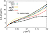Fig. 1. Energy per baryon of pure neutron matter as a function of the total baryon density at T = 0 MeV for all models considered in this work. Lines with stars indicate the overlapping region of several chiral-EFT calculations, taken from Huth et al. (2022).

In the top panel of Fig. 2 we plot the surface tension at β equilibrium for the representative temperature of T = 1 MeV, which is just above the expected crystallization temperature near the inner-crust bottom (see Carreau et al. 2020 and Dinh Thi et al. 2021, as well as our Fig. 7), for the two classes of RMF models, NL (solid lines) and DD (dashed lines). For comparison, the surface tension for a fixed proton fraction y_p = 0.3, a value close to the neutron drip line, is also shown. The difference between the two sets of curves (thick and thin lines) results from considering a DD proton fraction of heavy clusters (as obtained in β equilibrium) with respect to assuming a constant value (here, y_p = 0.3) in the surface tension. In the middle panel, for the same temperature and models, we show the proton fraction in the dense phase against the baryonic density obtained for β-equilibrated matter (thick lines) and matter with fixed proton fraction (thin lines). The global proton fraction at β equilibrium is plotted as a function of density in the bottom panel. As one can see from Eq. (34), the surface tension depends only on the cluster proton fraction, $y_p^I$. The strong decrease in the surface energy with density thus reflects the increasing neutron richness of the equilibrium nucleus, which in turn is due to the decreasing global proton fraction as a function of density (see the bottom panel). This general feature, as well as the disappearance of the surface tension at the crust–core transition, is common to all models. This behavior is in contrast to the case of a constant proton fraction. There, the proton fraction of the nucleus decreases very slowly (see the middle panel), from ∼0.4 in the very low density limit to the global value, 0.3, close to the dissolution of the clusters. This behavior is in turn reflected in the surface tension (see the top panel).

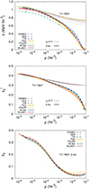Fig. 2. Cluster surface tension, σ (top panel), proton fraction in the dense phase, $y_p^I$ (middle panel), and global proton fraction, yp (bottom panel) in the inner crust at T = 1 MeV as a function of the total baryon density, ρ, obtained for β-equilibrated matter (thick lines) and matter with fixed proton fraction yp = 0.3 (thin lines in the top and middle panels) for all models considered in this work. The results are obtained without the translational term and the surface parameters are obtained from the fit to the mass table AME2016 (Audi et al. 2017).

In Fig. 3 we plot the absolute value of the ratio between the translational free energy term and the sum of the Coulomb and surface terms. Again, the specificity of the NS crust governed by β equilibrium (thick lines) can be appreciated from the comparison with the fixed proton fraction case, also shown in the figure (thin lines). In the β-equilibrium case, from the very low density limit up to ∼0.03 fm⁻³, the translational free energy term (with or without considering an effective mass number of the cluster) is much smaller than the sum of the Coulomb and surface terms. If the proton fraction of the droplet does not vary much with density, as is the case for y_p = 0.3, the translational term in the inner crust becomes completely negligible, particularly for ρ≳0.01 fm⁻³, at least at the relatively low temperatures corresponding to crustal crystallization. However, the effect is reversed in the innermost part of the inner crust when the β equilibrium is considered, which is due to the strong decrease in the surface tension in the very neutron-rich β-equilibrated matter observed in Fig. 2. This is in line with the results shown in Dinh Thi et al. (2023b, see their Fig. 6). As discussed at length in that work, in the global minimization of the cell free energy, the Coulomb plus surface term tends to favor the low-energy configurations as it is the case at T = 0, corresponding to highly bound heavy clusters. Conversely, the translational term tends to favor high-entropy configurations as in a classical gas, corresponding to small mass numbers for the droplet. The increase in the ratio between the two terms at high density means that heavy clusters are going to melt in the dense medium in a much more effective way when this term is accounted for.

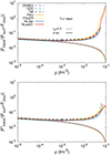Fig. 3. Absolute value of the translational free energy divided by the sum of the Coulomb and surface-energy terms as a function of the total baryon density, ρ, obtained in a CLD calculation with five light clusters at T = 1 MeV in β-equilibrated matter (thick lines) and matter with fixed proton fraction yp = 0.3 (thin lines) for all models considered in this work. The top (bottom) panel is obtained with the translational term of ideal gas, Ftrans (with the corrections on finite-size and in-medium effects, $F_{\mathrm{trans}}^{★}$).

This simplified picture occurs if we neglect the effect of the dripped neutrons on the translational motion of the droplet. With the inclusion of the effective mass number for the cluster, the translational degree of freedom is reduced in the dense medium, thus lowering this ratio and moderating the effect. Still, the impact of including the translational degrees of freedom in the variational equations is very important, as it can be seen from Fig. 4. Indeed, in this figure, we show how the number of protons (left panels) and nucleons (right panels) in the heavy cluster evolves with density, at the fixed temperature of T = 1 MeV. We only show the FSU and DD2 models, but the qualitative results are the same for all models used in this work. We considered three different cases: (i) without translational free energy (violet lines), (ii) with the translational free energy considering its ideal-gas version (green lines), and (iii) with the translational free energy and including the effective mass number of the cluster (black lines). The composition of matter in the NS crust (lower panels, β equilibrium) is very different from the case of dilute nuclear matter at constant proton fraction (upper panels). Looking at the top panels, the two models and the three different calculations behave similarly: the number of protons and of nucleons increase until the homogeneous matter is achieved. For the β-equilibrium calculations (bottom panels), the behavior is different: for both models, when the translational term is neglected (violet lines), the composition of the liquid crust is very close to what is expected for catalyzed ground-state composition, with an atomic number slowly varying according to the crustal depth, in the range Z_heavy≈30−40 (left panel), a faster increase in the nucleon number, in the range A_heavy≈100−400 (right panel), and a sharp increase in Z and A at the crust–core transition where matter becomes homogeneous. The difference between including or not the effective mass number in the translational term, that is, the difference between considering $F_{\mathrm{trans}}^{*}$, Eq. (39), instead of F_trans, Eq. (37), is to make the decrease in the droplet proton and nucleon numbers smoother. With the effective translational energy term (black lines), and for densities above ∼0.06 fm⁻³, the behavior of FSU is similar to the case without F_trans: the number of protons and of nucleons increases at the crust–core transition where the clusters dissolve. The DD2 model follows a different trend and does not show a steep increase at the crust–core transition. No heavy droplets survive at T = 1 MeV above a density of ρ≈0.04−0.05 fm⁻³ using F_trans, as we can see from the bottom left panel (green lines). This is because the effective number of nucleons has a strong correlation with the density of the neutron gas ${\rho }_n^{\mathit{II}}$ (recalling that $A^{*}=A_{\mathrm{heavy}}(1-{\rho }_n^{\mathit{II}}/{\rho }^I)=V^I({\rho }^I-{\rho }_n^{\mathit{II}})$). In β equilibrium, this quantity is quite high and close to the density of the cluster, when the baryonic density approaches the dissolution density of the clusters, making the cluster size to further decrease, $V^I=f{V}_W^{*}(1-f^{(1/3)}{)}^{-3}$. This is in line with Dinh Thi et al. (2023b, see their Figs. 7, 9, and 11).

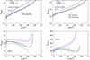Fig. 4. Number of protons (left) and nucleons (right) in the heavy cluster as a function of the total baryon density, ρ, in a CLD calculation with five light clusters for the FSU (solid lines) and DD2 (dashed lines) interactions with a fixed proton fraction of yp = 0.3 (top panels) and β equilibrium (bottom panels), at T = 1 MeV. The different colors represent the results obtained without the translational free energy (violet lines), with the ideal-gas translational term, Ftrans (green lines), and the corrected translational term, $F_{\mathrm{trans}}^{★}$ (black lines).

In Fig. 5 we show the mass fractions as a function of density for the light (top panel), and heavy (middle panel) clusters, together with the unbound nucleons (bottom panel). We only considered the most realistic prescription for the translational term with the effective mass number of the cluster, Eq. (39), and both NL (solid lines) and DD (dashed lines) models at the representative temperature of T = 1 MeV. The abundance of light clusters is systematically more important in the case of NL models, but it is globally small for all models, particularly in the inner-crust region. This can be understood from the fact that the mass fraction of the heavy clusters dominates in most of the crust, implying that the volume fraction of dilute matter is too small to accommodate an important contribution of light composites together with unbound neutrons. Compared to Dinh Thi et al. (2023a), where a full multicomponent plasma calculation suggested a dominance of He and Li isotopes in the innermost part of the inner crust, we observe that in that study these clusters were extremely neutron-rich, with mass numbers on the order of A_heavy≈20.

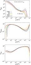Fig. 5. Mass fractions of light clusters (top panel), heavy clusters (middle panel), and unbound nucleons (bottom panel) as a function of the total baryon density, ρ, in the inner crust at T = 1 MeV for all models considered in this work. The results were obtained employing the corrected translational free energy, $F_{\mathrm{trans}}^{★}$.

We turn now to the discussion of the impurity parameter. In Fig. 6 we show the impurity parameter calculated at T = 1 MeV (top panel), 0.5 MeV (middle panel), and at the crystallization temperature T=T_melt (bottom panel), estimated in the one-component plasma approximation as (Haensel et al. 2007)

$$T_{\mathrm{melt}}=\frac{Z_{\mathrm{heavy}}^2{e}^2}{175\hspace{0.5em}{R}_W},$$(68)

with Z_heavy and R_W computed from a CLD calculation at T = 0 and in β equilibrium. The crystallization temperature is plotted as a function of the density in Fig. 7. To explore the variability of the impurity parameter with the temperature, we calculated it, as in previous works (Fantina et al. 2020; Carreau et al. 2020; Dinh Thi et al. 2023a), at different temperatures around T_melt (see Figs. 6 and 8). We notice that, as the density increases, the DD models present a lower impurity parameter as compared to the NL models. This is due to the fact that for the DD models the light-cluster mass fractions is lower, as can be seen in Fig. 5. Also, when we decrease the temperature to 0.5 MeV, the Q_imp values are much lower, especially for the DD models. The same happens when we calculate this parameter at the crystallization temperature: indeed, this quantity is essentially zero for the DD models, since already at T = 0.5 MeV and ρ≳0.01 fm⁻³, Q_imp≲10⁻⁸ (see the middle panel of Fig. 6), and T_melt≳0.5 MeV for ρ≳0.04 fm⁻³ (see Fig. 7). For the NL models, Q_imp takes also very small values: Q_imp∼10⁻⁶ at ρ∼10⁻² fm⁻³. We also notice that as the temperature decreases, the peak reached for each model decreases in magnitude but it happens at about the same density, as we can see from Fig. 8. This is very different from the results found in Dinh Thi et al. (2023a, see their Fig. 15), where light H and He isotopes were not considered, but a full multicomponent plasma calculation was performed accounting for fluctuations of the heavy cluster. Indeed, in Dinh Thi et al. (2023a), the change in temperature does not seem to particularly affect the amplitude of the maximum of Q_imp, but it shifts the density at which the peak occurs.

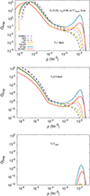Fig. 6. Impurity parameter, Qimp, as a function of the total baryon density, ρ, in a CLD calculation with five light clusters for all models considered in this work in β equilibrium and at T = 1 MeV (top panel), T = 0.5 (middle panel), and at the crystallization temperature, Tmelt (bottom panel). Results were obtained employing the corrected translational free energy, $F_{\mathrm{trans}}^{★}$.

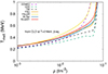Fig. 7. Crystallization temperature, Tmelt, as a function of the total baryon density, ρ, with Zheavy and RW obtained in a CLD calculation at T = 0 and β equilibrium for all models considered in this work.

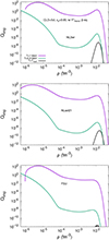Fig. 8. Impurity parameter, Qimp, as a function of the total baryon density, ρ, in a CLD calculation with five light clusters at β equilibrium for T = 1 MeV (violet lines), T = 0.5 MeV (green lines), and T=Tmelt (black lines), for NL3ωρ (top panel), NLset21 (middle panel), and FSU (bottom panel). Results were obtained employing the corrected translational free energy, $F_{\mathrm{trans}}^{★}$.

4. Conclusions

In this study we calculated the abundance of light clusters (namely, different non-exotic isotopes of H and He such as deuterons, tritons, ³He, α particles, and ⁶He) in thermodynamic conditions corresponding to the crystallization of the NS crust, using different RMF models and treating the light composites as independent structure-less quasi-particles. Such light clusters are expected to be formed in the dilute nucleon gas that characterizes the inner crust of the star while still in the liquid phase. The purpose of this study was to quantify the possible contribution due to such composite particles to the impurity factor that determines the resistivity of the NS crust, independently from the impact of a nuclear distribution that includes heavier and neutron-rich “exotic” light clusters, as addressed in previous works (Dinh Thi et al. 2023a).

In all models considered here, the contribution to the impurity factor that can be attributed to the presence of light clusters is negligible. This means that stable H and He clusters can be safely neglected and that the nucleon fluid made of dripped neutrons and protons in the inner crust can be treated as a homogeneous fluid, like in the mean-field approximation. As a consequence, we can conclude that, if high Q_imp values exist in the inner crust, as is suggested by different astrophysical observations (Pons et al. 2013; Newton 2013; Deibel et al. 2017; Hambaryan et al. 2017; Tan et al. 2018), its microscopic origin is likely due to the presence of either a deformed pasta mantle with defects (Schneider et al. 2014; Horowitz et al. 2015; Caplan et al. 2021; Newton et al. 2022) or to fluctuations in the charge of the dominant (heavy) ion in each cell (Carreau et al. 2020; Fantina et al. 2020; Dinh Thi et al. 2023a).

To definitively assess the possibility of multimode distributions of heavy ions with the emergence of (exotic) light droplets, the same multicomponent treatment of Dinh Thi et al. (2023a) should be employed, together with microscopic many-body approaches based on the density-functional formalism for the ion energy that consider realistic nucleon density profiles. These methods, which are, however, computationally more expensive, include Hartree-Fock-Bogoliubov and (extended) Thomas-Fermi approaches (see, e.g., Newton & Stone 2009; Onsi et al. 2008; Shchechilin et al. 2024).

Acknowledgments

This work was partially supported by national funds from FCT (Fundação para a Ciência e a Tecnologia, I.P, Portugal) under projects UIDB/04564/2020 and UIDP/04564/2020, with DOI identifiers 10.54499/UIDB/04564/2020 and 10.54499/UIDP/04564/2020, respectively, and the project 2022.06460.PTDC with the associated DOI identifier 10.54499/2022.06460.PTDC. H.P. acknowledges the grant 2022.03966.CEECIND (FCT, Portugal) with DOI identifier 10.54499/2022.03966.CEECIND/CP1714/CT0004. F.G., A.F. and H.D.T. ackowledge the support by the IN2P3 Master Project NewMAC and MAC, the ANR project ‘Gravitational waves from hot neutron stars and properties of ultra-dense matter’ (GW-HNS, ANR-22-CE31-0001-01), the CNRS International Research Project (IRP) ‘Origine des éléments lourds dans l’univers: Astres Compacts et Nucléosynthèse (ACNu)’.

References

All Tables

All Figures

	Fig. 1. Energy per baryon of pure neutron matter as a function of the total baryon density at T = 0 MeV for all models considered in this work. Lines with stars indicate the overlapping region of several chiral-EFT calculations, taken from Huth et al. (2022).
In the text

Fig. 2. Cluster surface tension, σ (top panel), proton fraction in the dense phase, $y_p^I$ (middle panel), and global proton fraction, yp (bottom panel) in the inner crust at T = 1 MeV as a function of the total baryon density, ρ, obtained for β-equilibrated matter (thick lines) and matter with fixed proton fraction yp = 0.3 (thin lines in the top and middle panels) for all models considered in this work. The results are obtained without the translational term and the surface parameters are obtained from the fit to the mass table AME2016 (Audi et al. 2017).

In the text

Fig. 3. Absolute value of the translational free energy divided by the sum of the Coulomb and surface-energy terms as a function of the total baryon density, ρ, obtained in a CLD calculation with five light clusters at T = 1 MeV in β-equilibrated matter (thick lines) and matter with fixed proton fraction yp = 0.3 (thin lines) for all models considered in this work. The top (bottom) panel is obtained with the translational term of ideal gas, Ftrans (with the corrections on finite-size and in-medium effects, $F_{\mathrm{trans}}^{★}$).

In the text

Fig. 4. Number of protons (left) and nucleons (right) in the heavy cluster as a function of the total baryon density, ρ, in a CLD calculation with five light clusters for the FSU (solid lines) and DD2 (dashed lines) interactions with a fixed proton fraction of yp = 0.3 (top panels) and β equilibrium (bottom panels), at T = 1 MeV. The different colors represent the results obtained without the translational free energy (violet lines), with the ideal-gas translational term, Ftrans (green lines), and the corrected translational term, $F_{\mathrm{trans}}^{★}$ (black lines).

In the text

	Fig. 5. Mass fractions of light clusters (top panel), heavy clusters (middle panel), and unbound nucleons (bottom panel) as a function of the total baryon density, ρ, in the inner crust at T = 1 MeV for all models considered in this work. The results were obtained employing the corrected translational free energy, $F_{\mathrm{trans}}^{★}$.
In the text

	Fig. 6. Impurity parameter, Qimp, as a function of the total baryon density, ρ, in a CLD calculation with five light clusters for all models considered in this work in β equilibrium and at T = 1 MeV (top panel), T = 0.5 (middle panel), and at the crystallization temperature, Tmelt (bottom panel). Results were obtained employing the corrected translational free energy, $F_{\mathrm{trans}}^{★}$.
In the text

	Fig. 7. Crystallization temperature, Tmelt, as a function of the total baryon density, ρ, with Zheavy and RW obtained in a CLD calculation at T = 0 and β equilibrium for all models considered in this work.
In the text

	Fig. 8. Impurity parameter, Qimp, as a function of the total baryon density, ρ, in a CLD calculation with five light clusters at β equilibrium for T = 1 MeV (violet lines), T = 0.5 MeV (green lines), and T=Tmelt (black lines), for NL3ωρ (top panel), NLset21 (middle panel), and FSU (bottom panel). Results were obtained employing the corrected translational free energy, $F_{\mathrm{trans}}^{★}$.
In the text

References

- Arcones, A., Martinez-Pinedo, G., O’Connor, E., et al. 2008, Phys. Rev. C, 78, 015806 [NASA ADS] [CrossRef] [Google Scholar]
- Audi, G., Kondev, F. G., Wang, M., Huang, W. J., & Naimi, S. 2017, Chin. Phys. C, 41, 030001 [NASA ADS] [CrossRef] [Google Scholar]
- Avancini, S. S., Barros, C. C. Jr., Brito, L., et al. 2012, Phys. Rev. C, 85, 035806 [Google Scholar]
- Bao, S. S., Hu, J. N., Zhang, Z. W., & Shen, H. 2014, Phys. Rev. C, 90, 045802 [NASA ADS] [CrossRef] [Google Scholar]
- Bauswein, A., Goriely, S., & Janka, H. T. 2013, ApJ, 773, 78 [NASA ADS] [CrossRef] [Google Scholar]
- Baym, G., Bethe, H. A., & Pethick, C. 1971, Nucl. Phys. A, 175, 225 [NASA ADS] [CrossRef] [Google Scholar]
- Bougault, R., Bonnet, E., Borderie, B., et al. 2020, J. Phys. G, 47, 025103 [NASA ADS] [CrossRef] [Google Scholar]
- Camelio, G., Lovato, A., Gualtieri, L., et al. 2017, Phys. Rev. D, 96, 043015 [Google Scholar]
- Caplan, M. E., Forsman, C. R., & Schneider, A. S. 2021, Phys. Rev. C, 103, 055810 [NASA ADS] [CrossRef] [Google Scholar]
- Carreau, T., Fantina, A. F., & Gulminelli, F. 2020, A&A, 640, A77, [Erratum: A&A 645, C1 (2021)] [NASA ADS] [CrossRef] [EDP Sciences] [Google Scholar]
- Custódio, T., Falcão, A., Pais, H., et al. 2020, Eur. Phys. J. A, 56, 295 [Google Scholar]
- Custódio, T., Rebillard-Soulié, A., Bougault, R., et al. 2024, arXiv e-prints [2407.02307] [Google Scholar]
- Deibel, A., Cumming, A., Brown, E. F., & Reddy, S. 2017, ApJ, 839, 95 [Google Scholar]
- Dinh Thi, H., Fantina, A. F., & Gulminelli, F. 2021, Eur. Phys. J. A, 57, 296 [NASA ADS] [CrossRef] [Google Scholar]
- Dinh Thi, H., Fantina, A. F., & Gulminelli, F. 2023a, A&A, 677, A174 [NASA ADS] [CrossRef] [EDP Sciences] [Google Scholar]
- Dinh Thi, H., Fantina, A. F., & Gulminelli, F. 2023b, A&A, 672, A160 [NASA ADS] [CrossRef] [EDP Sciences] [Google Scholar]
- Fantina, A. F., De Ridder, S., Chamel, N., & Gulminelli, F. 2020, A&A, 633, A149 [NASA ADS] [CrossRef] [EDP Sciences] [Google Scholar]
- Ferreira, M., & Providencia, C. 2012, Phys. Rev. C, 85, 055811 [NASA ADS] [CrossRef] [Google Scholar]
- Fischer, T., Hempel, M., Sagert, I., Suwa, Y., & Schaffner-Bielich, J. 2014, Eur. Phys. J. A, 50, 46 [NASA ADS] [CrossRef] [Google Scholar]
- Fischer, T., Typel, S., Röpke, G., Bastian, N. -U. F., & Martínez-Pinedo, G. 2020, Phys. Rev. C, 102, 055807 [NASA ADS] [CrossRef] [Google Scholar]
- Furnstahl, R. J., Serot, B. D., & Tang, H. -B. 1996, Nucl. Phys. A, 598, 539 [Google Scholar]
- Furnstahl, R. J., Serot, B. D., & Tang, H. B. 1997, Nucl. Phys. A, 615, 441, [Erratum: Nucl.Phys.A 640, 505–505 (1998)] [Google Scholar]
- Furusawa, S., Nagakura, H., Sumiyoshi, K., & Yamada, S. 2013, ApJ, 774, 78 [Google Scholar]
- Furusawa, S., Sumiyoshi, K., Yamada, S., & Suzuki, H. 2017, Nucl. Phys. A, 957, 188 [Google Scholar]
- Goriely, S., Chamel, N., Janka, H. T., & Pearson, J. M. 2011, A&A, 531, A78 [NASA ADS] [CrossRef] [EDP Sciences] [Google Scholar]
- Grill, F., Pais, H., Providência, C., Vidaña, I., & Avancini, S. S. 2014, Phys. Rev. C, 90, 045803 [NASA ADS] [CrossRef] [Google Scholar]
- Haensel, P., Potekhin, A. Y., & Yakovlev, D. G. 2007, Neutron stars 1: Equation of state and structure (New York, USA: Springer), 326 [Google Scholar]
- Hagen, G. A., Ekström, A., Forssén, C., et al. 2015, Nat. Phys., 12, 186 [Google Scholar]
- Hambaryan, V., Suleimanov, V., Haberl, F., et al. 2017, A&A, 601, A108 [NASA ADS] [CrossRef] [EDP Sciences] [Google Scholar]
- Horowitz, C. J., & Piekarewicz, J. 2001, Phys. Rev. Lett., 86, 5647 [NASA ADS] [CrossRef] [Google Scholar]
- Horowitz, C. J., Berry, D. K., Briggs, C. M., et al. 2015, Phys. Rev. Lett., 114, 031102 [NASA ADS] [CrossRef] [Google Scholar]
- Huth, S., Pang, P. T. H., Tews, I., et al. 2022, Nature, 606, 276 [CrossRef] [PubMed] [Google Scholar]
- Lalazissis, G. A., Nikšć, T., Vretenar, D., & Ring, P. 2005, Phys. Rev. C, 71, 024312 [NASA ADS] [CrossRef] [Google Scholar]
- Lattimer, J. M., & Swesty, F. D. 1991, Nucl. Phys. A, 535, 331 [CrossRef] [Google Scholar]
- Lattimer, J. M., Pethick, C. J., Ravenhall, D. G., & Lamb, D. Q. 1985, Nucl. Phys. A, 432, 646 [NASA ADS] [CrossRef] [Google Scholar]
- Magierski, P., & Bulgac, A. 2004, Nucl. Phys. A, 738, 143 [NASA ADS] [CrossRef] [Google Scholar]
- Malik, T., & Providência, C. 2022, Phys. Rev. D, 106, 063024 [NASA ADS] [CrossRef] [Google Scholar]
- Malik, T., Pais, H., & Providência, C. 2024, A&A, 689, A242 [NASA ADS] [CrossRef] [EDP Sciences] [Google Scholar]
- Martin, N., & Urban, M. 2016, Phys. Rev. C, 94, 065801 [NASA ADS] [CrossRef] [Google Scholar]
- Nedora, V., Bernuzzi, S., Radice, D., et al. 2021, ApJ, 906, 98 [NASA ADS] [CrossRef] [Google Scholar]
- Negreiros, R., Tolos, L., Centelles, M., Ramos, A., & Dexheimer, V. 2018, ApJ, 863, 104 [Google Scholar]
- Newton, W. G. 2013, Nat. Phys., 9, 396 [CrossRef] [Google Scholar]
- Newton, W. G., & Stone, J. R. 2009, Phys. Rev. C, 79, 055801 [NASA ADS] [CrossRef] [Google Scholar]
- Newton, W. G., Kaltenborn, M. A., Cantu, S., et al. 2022, Phys. Rev. C, 105, 025806 [Google Scholar]
- Onsi, M., Dutta, A. K., Chatri, H., et al. 2008, Phys. Rev. C, 77, 065805 [NASA ADS] [CrossRef] [Google Scholar]
- Pais, H., & Providência, C. 2016, Phys. Rev. C, 94, 015808 [NASA ADS] [CrossRef] [Google Scholar]
- Pais, H., Chiacchiera, S., & Providência, C. 2015, Phys. Rev. C, 91, 055801 [NASA ADS] [CrossRef] [Google Scholar]
- Pais, H., Gulminelli, F., Providência, C., & Röpke, G. 2018, Phys. Rev. C, 97, 045805 [NASA ADS] [CrossRef] [Google Scholar]
- Pais, H., Gulminelli, F., Providência, C., & Röpke, G. 2019, Phys. Rev. C, 99, 055806 [Google Scholar]
- Pais, H., Bougault, R., Gulminelli, F., et al. 2020, Phys. Rev. Lett., 125, 012701 [CrossRef] [Google Scholar]
- Pons, J. A., Vigano’, D., & Rea, N. 2013, Nat. Phys., 9, 431 [NASA ADS] [CrossRef] [Google Scholar]
- Potekhin, A. Y., & Chabrier, G. 2000, Phys. Rev. E, 62, 8554 [NASA ADS] [CrossRef] [Google Scholar]
- Potekhin, A. Y., & Chabrier, G. 2021, A&A, 645, A102 [NASA ADS] [CrossRef] [EDP Sciences] [Google Scholar]
- Psaltis, A., Jacobi, M., Montes, F., et al. 2024, ApJ, 966, 11 [Google Scholar]
- Qin, L., Hagel, K., Wada, R., et al. 2012, Phys. Rev. Lett., 108, 172701 [CrossRef] [Google Scholar]
- Radice, D., Perego, A., Hotokezaka, K., et al. 2018, ApJ, 869, 130 [Google Scholar]
- Ren, Z., Elhatisari, S., Lähde, T. A., Lee, D., & Meißner, U. -G. 2024, Phys. Lett. B, 850, 138463 [Google Scholar]
- Röpke, G. 2015, Phys. Rev. C, 92, 054001 [CrossRef] [Google Scholar]
- Röpke, G. 2020, Phys. Rev. C, 101, 064310 [CrossRef] [Google Scholar]
- Rosswog, S. 2015, Int. J. Mod. Phys. D, 24, 1530012 [NASA ADS] [CrossRef] [Google Scholar]
- Schneider, A. S., Berry, D. K., Briggs, C. M., Caplan, M. E., & Horowitz, C. J. 2014, Phys. Rev. C, 90, 055805 [Google Scholar]
- Sedrakian, A. D. 1996, Astrophys. Space Sci., 236, 267 [NASA ADS] [CrossRef] [Google Scholar]
- Shchechilin, N. N., Chamel, N., & Pearson, J. M. 2023, Phys. Rev. C, 108, 025805 [Google Scholar]
- Shchechilin, N. N., Chamel, N., Pearson, J. M., Chugunov, A. I., & Potekhin, A. Y. 2024, Phys. Rev. C, 109, 055802 [Google Scholar]
- Sumiyoshi, K., & Roepke, G. 2008, Phys. Rev. C, 77, 055804 [Google Scholar]
- Tan, C. M., Bassa, C. G., Cooper, S., et al. 2018, ApJ, 866, 54 [NASA ADS] [CrossRef] [Google Scholar]
- Todd-Rutel, B. G., & Piekarewicz, J. 2005, Phys. Rev. Lett., 95, 122501 [NASA ADS] [CrossRef] [Google Scholar]
- Typel, S., & Wolter, H. H. 1999, Nucl. Phys. A, 656, 331 [Google Scholar]
- Typel, S., Ropke, G., Klahn, T., Blaschke, D., & Wolter, H. H. 2010, Phys. Rev. C, 81, 015803 [Google Scholar]
- Viganò, D., Rea, N., Pons, J. A., et al. 2013, MNRAS, 434, 123 [CrossRef] [Google Scholar]
All Tables
Optimized surface parameters, namely σ0, bs, and p, for the models considered in this work, fitted to the AME2016 mass table.