| Issue |
A&A
Volume 699, July 2025
|
|
|---|---|---|
| Article Number | A241 | |
| Number of page(s) | 18 | |
| Section | Astronomical instrumentation | |
| DOI | https://doi.org/10.1051/0004-6361/202553726 | |
| Published online | 11 July 2025 | |
The near-infrared airglow continuum conundrum
Constraints for ground-based faint object spectroscopy
1
Cosmic Dawn Center (DAWN),
Denmark
2
Niels Bohr Institute, University of Copenhagen,
Jagtvej 155A,
2200
Copenhagen N,
Denmark
3
Nordic Optical Telescope,
Rambla José Ana Fernández Pérez 7,
38711
Breña Baja,
Spain
4
Department of Physics and Astronomy, Aarhus University,
Munkegade 120,
8000
Aarhus C,
Denmark
★ Corresponding author: This email address is being protected from spambots. You need JavaScript enabled to view it.
Received:
10
January
2025
Accepted:
31
May
2025
Abstract
Context. The airglow continuum in the near-infrared is challenging to quantify due to its faintness and the grating-scattered light from atmospheric hydroxyl (OH) emission lines. Despite its faintness, the airglow continuum sets fundamental limits for ground-based spectroscopy of faint targets and accounts for the difference between ground- and space-based observations in the interline regions between atmospheric emission lines.
Aims. We aim to quantify the level of airglow continuum radiance in the visible- to near-infrared wavelength range observable with silicon photodetectors at the Observatorio del Roque de los Muchachos, in such a way that our measurement is not biased by the grating-scattered light. We aim to do this by measuring the airglow continuum radiance with minimal and controlled contamination from the broad instrumental scattering wings caused by the bright atmospheric OH lines.
Methods. We measured the airglow continuum radiance using a long-slit λ/Δλ ~ 4000 spectrograph in ~100 Å-wide narrow bandpasses centered at 6720, 7700, 8700, and 10 500 Å (corresponding to the R, I, and Z broadbands) with the 2.5-meter Nordic Optical Telescope under photometric dark-sky conditions. The bandpasses were chosen to be as free as possible from atmospheric absorption and OH line emission, thereby minimizing the radiation reaching the grating surface.
Results. We observe the zenith-equivalent airglow continuum to be 22.5 mag arcsec−2 at 6720 Å and 22 mag arcsec−2 at 8700 Å. We derive upper limits of 22 mag arcsec−2 at 7700 Å, due to difficulties in finding a clean part of the spectrum for measurement, and 20.8 mag arcsec−2 at 10 500 Å, due to low system sensitivity. Within measurement errors and the natural variability expected for airglow emission, our results for the Observatorio del Roque de los Muchachos are comparable to the values reported for other major observatory sites. With our medium-resolution spectra, we are unable to comment on the origin of the radiance, which could still be due to faint unresolved spectral lines or the true (pseudo)continuum. The measurement uncertainty on the zenith-scaled continuum radiance is dominated by detector effects, assumptions on atmospheric scattering, and the choice of zodiacal light model.
Conclusions. We conclude that the airglow continuum radiance is not due to instrumental effects in our bandpasses and measure it to be two to four times brighter than the zodiacal light toward the ecliptic poles, the darkest foreground available for both ground- and space-based observatories. While the level is not negligible, it is dark enough to encourage further investigations into novel optical technologies and apply known stray light reduction techniques to future near-infrared and short-wave infrared spectroscopic instrumentation.
Key words: atmospheric effects / instrumentation: spectrographs / methods: observational / infrared: diffuse background
© The Authors 2025
 Open Access article, published by EDP Sciences, under the terms of the Creative Commons Attribution License (https://creativecommons.org/licenses/by/4.0), which permits unrestricted use, distribution, and reproduction in any medium, provided the original work is properly cited.
This article is published in open access under the Subscribe to Open model. This email address is being protected from spambots. You need JavaScript enabled to view it. to support open access publication.
1 Introduction
Astronomy has entered the photon noise-limited era, driven by even lower-noise photodetectors and larger aperture telescopes, as highlighted by the forthcoming extremely large telescopes (ELTs). Both ground- and space-based observatories are affected by the zodiacal light (ZL), while ground-based facilities experience additional emission from the foreground sky, the continuum radiance of which is still not well understood. To set a reference for the foreground brightness, the darkest VIS–NIR1 foreground available from both ground and space is toward the ecliptic poles, making them ideal zones for deep fields such as the Hubble deep field (HDF; Williams et al. 1996) and the Great Observatories Origins Deep Survey (GOODS; Giavalisco et al. 2004) fields. The yearly average ZL foreground in HDF is ~50 ph s−1m−2μm−1arcsec−2 at 1.25 μm, corresponding to 22.4 mag arcsec−2. Similarly, the cosmic evolution survey (COSMOS; Scoville et al. 2007; Weaver et al. 2022) field, located at a lower ecliptic latitude, βec = −9°, offers a background of ~85 ph s−1m−2μm−1arcsec−2 or 21.8 mag arcsec−2 for the darkest part of the year but undergoes large variation depending on the Solar elongation angle. Ground-based astronomical observatories are located at some of the darkest sites around the globe, with typical broadband sky brightness ranging in the visual (VIS) V ~ 22 mag arcsec−2, but rapidly increasing toward longer wavelengths, reaching I ~ 20 mag arcsec−2 in NIR, and J ~ 16 mag−2 arcsec−2, H ~ 14 mag arcsec−2 in SWIR. The reason for the increase is the radiance from the increasing number density and brightness of rotation-vibrational transitions of hydroxyl (OH) molecules, and to a lesser extent molecular oxygen O2. The behavior of atmospheric line emission is understood to a level where sophisticated models have been developed (e.g., ESO SkyCalc, Noll et al. 2012; Jones et al. 2013). However, the interline airglow continuum emission, especially in NIR–SWIR wavelengths, remains much less well known due to its faintness and the challenges of its measurement. Instrumental effects, such as grating-scattered light and thermal stray light, complicate the airglow continuum measurement if the experiment is not carefully designed.
Published, dedicated airglow continuum radiance measurements at VIS and NIR wavelengths are mainly from the 1960s and 1970s (Krassovsky et al. 1962; Broadfoot & Kendall 1968; Sternberg & Ingham 1972; Gadsden & Marovich 1973; Noxon 1978; Sobolev 1978). Since then, the VIS and NIR continuum radiance has been studied at Cerro Paranal, Chile (Hanuschik 2003; Patat 2008; Noll et al. 2024). After the introduction of SWIR mercury-cadmium-telluride detectors, the interest in airglow continuum radiance shifted mostly to SWIR (Maihara et al. 1993b; Cuby et al. 2000; Ellis et al. 2012; Sullivan & Simcoe 2012; Trinh et al. 2013; Oliva et al. 2015; Nguyen et al. 2016), where the ZL foreground is significantly lower than in NIR (Leinert et al. 1998; Windhorst et al. 2022). Special attention has been given to a relatively narrow spectral region in the H band located around 16 650 Å, originally selected by Maihara et al. (1993b), despite later studies finding few emission lines in this region (Oliva et al. 2015). We summarize previous airglow continuum measurements found in the literature in Table B.1.
Both spectroscopic and narrow-band imaging measurements have been done to determine the airglow continuum radiance in the NIR and SWIR range. Both methods have their advantages and disadvantages: it is difficult to find a clean spectral bandpass without airglow emission lines for narrow-band imaging, and grating spectrographs are susceptible to suffering from grating-scattered light, which can appear as dislocated copies of a parent line and broad diffuse line wings (Woods et al. 1994; Koch et al. 2021). In NIR and SWIR wavelengths, the scattered light combined from all airglow emission lines can result in an artificial continuum (Ellis & Bland-Hawthorn 2008; Sullivan & Simcoe 2012; Oliva et al. 2015). Sullivan & Simcoe (2012) concluded that their continuum measurement in the H band could be explained by the spectrograph’s line spread function (LSF) wings, while shorter wavelength bands remain unaffected. Thermal blackbody radiation from the instrument may additionally affect the measurement (Ellis et al. 2020). To minimize the effect of grating-scattered light, a number of spectroscopic measurements in the 1–2 μm range have been accompanied by OH line emission suppression units (e.g., Maihara et al. 1993a; Ellis et al. 2012).
A further complication is that airglow exhibits significant temporal variation, with timescales ranging from minutes (due to mesospheric buoyancy waves) (Smith et al. 2006; Moreels et al. 2008), to years (Solar cycle) (Leinert et al. 1995; Mattila et al. 1996; Krisciunas 1997; Patat 2008; Noll et al. 2017). Additionally, semiannual (Grygalashvyly et al. 2021) and diurnal variability (Smith 2012) of the line emission is present. The airglow continuum has been observed to exhibit diurnal variability (Trinh et al. 2013). The NIR and SWIR OH and O2 line emissions are known to originate from the mesopause region (e.g., Baker & Stair 1988). There is a strong density change in the mesopause, and waves can travel at the boundary layer. Typically, these gravity or buoyancy waves can be observed with a ~15% brightness variation on timescales from a few up to tens of minutes (Moreels et al. 2008). However, mesospheric bore events can drive solitons, which may cause sudden, localized, large-amplitude changes (e.g., Smith et al. 2006).
Despite the challenges in measurement, a number of chemiluminescent processes are known to contribute to the atmospheric continuum radiance. Several nitrogen monoxide (NO) reactions are known to contribute to the total VIS–NIR continuum (see Bates 1993; Khomich et al. 2008; Noll et al. 2024, and references therein for extended discussion). However, none of the reactions have a rate that is sufficiently high to explain the total continuum radiance that has been observed. Recently, it has been shown that iron monoxide (FeO) has an extended pseudocontinuum emission spectrum extending from VIS to SWIR, with the potential to explain a significant fraction of the VIS–NIR continuum emission (Noll et al. 2024). FeO still leaves a significant SWIR component unattributed, which is possibly due to hydroperoxyl HO2 (preprint, Noll et al. 2025).
The objective of this study is to measure the airglow continuum with a method that strongly reduces the effect of grating-scattered light. Our study is limited to the spectral range observable with a Charge-Coupled Device (CCD), i.e., below about 11 000 Å. The airglow spectra were observed through narrow band (NB) filters, which is not a full-fledged OH suppression scheme but allows for the selection of bandpasses such that the number and brightness of unwanted OH line emissions are kept to a minimum. Data recording is described in detail in Sect. 2. Due to the faint signal level, additional efforts were spent on reducing the data, which is discussed in Sect. 3. We compensated for the low sensitivity close to the detector sensitivity limit by observing thicker air columns, i.e., fields at very large zenith distances. The assumptions underlying our final results are discussed in the analysis Sect. 4. Lastly, the implications of our results are discussed in Sect. 5 and 6. Observed apparent airglow spectra are included in Appendix A. References to previous similar studies found in the literature are gathered in Appendix B, and their results are converted to the units used in this work to allow for comparison.
2 Observations and data
2.1 Site
We recorded airglow continuum spectra with the ALFOSC instrument mounted on the 2.56-meter Nordic Optical Telescope (NOT). The NOT is located at the Observatorio del Roque de los Muchachos on La Palma, Canary Islands, Spain, with the geographical coordinates +28°45′26.2″ N and 17°53′06.3″ W, and an altitude of 2382 meters. The NOT has a lower pointing limit of 6° above the horizon, and its location is such that the horizon is unobstructed when observing toward the north. The northern direction has the least amount of light pollution at the site, since the line of sight travels entirely above the Atlantic, with the only source of artificial illumination being the town of Roque del Faro, located 5 km north of the Observatorio del Roque de los Muchachos. Light pollution, which is mostly caused by low-pressure sodium lamps with characteristic wavelengths of 5890 and 5896 Å, falls outside the bandpasses in our study. The next source of artificial illumination on the line of sight is the island of Madeira, which is 450 km north of La Palma.
2.2 Field selection
The observed fields on the sky were chosen to be as dark as possible outside the atmosphere, away from both the ecliptic and galactic planes, and yet close to the horizon to be able to observe it with a thick air column. The COBE Diffuse Infrared Background Experiment (DIRBE) (Hauser et al. 1998; Arendt et al. 1998; Kelsall et al. 1998; Dwek et al. 1998) band 1 maps, with a central wavelength of 1.25 μm, were first used to locate fields with low surface brightness (Fig. 1). PanSTARRS DR1 z-band images (Flewelling et al. 2020) were then used to fine-tune the location to areas with the fewest visible sources and to assist in orienting the slit on the sky. To summarize, the coordinates for the pointings were chosen with the following selection criteria:
Ecliptic latitude βec > 50°;
DIRBE band 1 radiance < 85 ph s−1m−2μm−1arcsec−2;
No bright, m < 12 mag, stars in the 6.5′×6.5′ ALFOSC field of view;
No sources visible in the slit area in the PanSTARRS z-band image;
Observable with a zenith distance z > 75° toward the north; and
Only a few degrees variation in zenith distance during the measurement.
Additionally, the following time restrictions were adopted:
Moon altitude <−30°,
Moon separation >60°,
to ensure no scattered moonlight was observed (Krisciunas & Schaefer 1991; Jones et al. 2013). Typically, the Moon illumination fraction during our observations was <2%. Additionally, the first observing run was purposefully scheduled to coincide with the December solstice to provide the longest possible night. Observations typically occurred several hours after sunset, and in most cases past the local midnight.
Optical configurations used for the NB observations.
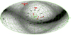 |
Fig. 1 Projection of the COBE/DIRBE band 1 map with a central wavelength at 1.25 μm toward the ecliptic north pole. The red markers indicate the coordinates for our pointings, the HDF, and the COSMOS field. The Milky Way crosses the map horizontally, while ZL in the ecliptic plane appears as a ring between declinations δ = [−30, 30]. |
2.3 Optical setup
The optical setups that were used are summarized in Table 1, with optical component names referring to the NOT’s optical element database. Four NB filters were purchased for the experiment, with spectral bandpasses chosen such that they would mostly be free from bright (OH) lines and atmospheric molecular absorption. The chosen bands were centered at 6720, 7700, 8700, and 10 500 Å (see Fig. 2). The bandpasses were generally clean of strong absorption, apart from the 7700 Å band, which has significant O2 absorption on the blue side of the bandpass. The bandpasses were 60–120 Å in width, limiting the total OH line flux reaching the grism to its minimum. All bright OH lines within the bandpasses were located in the wings of the NB filter transmission profiles. The NB filters were positioned in the beam before the grisms in the optical path; thus the stray light introduced by the OH lines were kept to a minimum.
The three redder NB filters had a diameter of 25.4 mm, which would significantly vignette the ALFOSC beam if placed in standard filter mounting slots, and were consequently mounted on the slit wheel instead. This reduced the effective slit length to 2.4′, allowing a sampling of 675 px on the detector with the reduced slit length. The vertical slits for the 6720 Å band were 5.3′in length, allowing a sampling of 1500 px. In the three reddest bands, the echelle grism #9 was used as the dispersive element, since it had the highest resolution of the available grisms, λ/Δλ ≈ 4300, with a spectral coverage up to the CCD sensitivity cutoff at 11 000 Å. The broadband SDSS i′ and z′ -filters were used for order sorting with grism #9. The 6720 Å and was observed with grism #17 using the Gunn r-band filter for order sorting. Using the order sorter was probably unnecessary with grism #17, but was done as a precaution.
The 2D spectrum was binned along the slit dimension before the readout and later during the analysis, and the entire remaining slit length was median-collapsed into 1D. This process has the potential to cause smearing and additional line broadening. To counter this, both the slits and the grisms were carefully aligned before the observation such that the slit and dispersion direction matched the detector pixel row and column axes to minimize smearing. Both were aligned to within less than one pixel RMS difference relative to the detector axes. Potential spread was negligible, and any possible resulting broadening was captured by the LSF model.
We checked the instrument pixel scale on a few denser standard star fields and find it to be constant over the field of view with a value of 0.21377 ± 5 × 10⁻⁵ arcsec px−1 by plate solving. Slit widths were measured by illuminating the slit with a standard calibration arc lamp, and by imaging them with the ALFOSC camera.
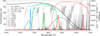 |
Fig. 2 Transmission curves of the NB filters, order-sorting broad-band filters, grism blaze functions, detector efficiency, and atmospheric transmission at the observed zenith distance. The blue half of the 7700 Å band is strongly absorbed by atmospheric O2. In the 10 500 Å band, the total system efficiency is very low, as the wavelength falls within the wing of the grism blaze function. |
2.4 Line spread function
The diffraction theory predicts a Lorentzian-like envelope for the grating distribution function, which is modulated by the spectrograph camera point spread function. For a good camera optic, the point spread function is approximately Gaussian. In addition to the Lorentzian and Gaussian components, the micro-roughness of the grating surface contributes a diffuse component (Woods et al. 1994; Koch et al. 2021). To estimate the wing contribution to the measured continua, a crude estimate of the LSF was made based on Thorium-Argon arc lamp exposures, since no monochromatic light source operating within the bandpasses was available. The approach was far from optimal, due to unresolved and too faint lamp lines, but was sufficient to derive an upper limit on the grating-scattered light. A combination of Lorentzian and Gaussian functions was fit on prominent arc lines visible in the bandpasses. Grism #17 was best fit with a function that was almost completely Lorentzian, whereas grism #9 appeared mainly Gaussian, which might indicate that the acquired arc exposures of grism #9 were not deep enough to expose the Lorentzian wings. However, this would lead to fitting the wings to the readout-noise floor, thereby further overestimating the scattering-wing contribution.
Based on the fits, 95% of the line flux is within ±0.5 Å, ±1.7 Å, and ±2.1 Å from the line center in the 6720, 7700, and 8700 Å bands, respectively. Similarly, 99% of the flux is within ±0.9 Å, ±6.7 Å, and ±6.6 Å. To give a gross overestimate of the LSF wing contribution, the remaining 1% of the light further from the core can be taken as the diffuse LSF component. Dividing the 1% of the total line flux in each band and distributing it equally within the full width at half maximum (FWHM) of the NB filter, one reaches an upper limit of 4×10⁻⁴, 0.2, and 0.1 e− px−1 in the 6720, 7700, and 8700 Å bands, respectively, which are well below the systematic uncertainty of 0.6 e− px−1 from bias subtraction (see Sect. 3). Consequently, we expect the OH-line wing contribution originating from the OH lines within the bandpass to the measured continuum to be negligible. Our measurement in the 10 500 Å band is detector-noise limited, and no continuum detection was achieved. Consequently, we did not study the effect of the LSF wings in this band.
2.5 Detector setup
The ALFOSC is equipped with a deep-depleted e2v CCD231-42 backside-illuminated CCD with active pixel dimensions of 2048 × 2064 px. Outside the image area, there is an additional 38 px of vertical and 2×50 px of horizontal overscan. The CCD controller has four readout amplifiers, with amplifiers B and D showing very similar performance. For an unknown reason, the binning for amplifier D limited the usable detector area, leading us to use amplifier B for the measurement. Additionally, amplifier B was located further away from the region of interest for the three reddest bands, giving the controller more time to stabilize during a readout. Based on NOT’s long-term quality control monitoring, the readout noise of amplifier B was 4.40 ± 3 × 10⁻² e− for the slowest available readout speed of 100 kHz. According to the same quality control data, the gain was 0.169 ± 2 × 10⁻³ e− ADU−1. These values are adopted in our analysis. Different binning factors were studied before beginning the observations, and a binning of 5 was adopted in the slit dimension.
Table of observations.
2.6 Atmospheric conditions
All observations were carried out under photometric conditions. The appearance of high clouds along the line of sight was monitored with all-sky cameras to ensure that a cloud layer would not interrupt our observations. Low dust particle counts, such as those caused by Calima from the Sahara (Murdin 1986), were measured at the level of the observatory during all nights. Tenerife, 130 km away, was clearly visible on all nights of observation, providing a VIS reference for atmospheric turbidity and indicating good atmospheric transparency.
The first set of observations was carried out on the nights of December 30, 2021, through January 2, 2022, and a second set of observations was performed in March 2023 (see the list of observations in Table 2). The main run took place one week after the winter December solstice, during dark-sky conditions with no Moon illumination. Observations were made between 00:00 UT and 02:00 UT at an altitude of 10° above the horizon to guarantee a thick air column and only a small amount of non-atmospheric emission. The horizon was clear during all four December nights, and observing conditions were generally excellent. Additional observations were carried out in September 2024, again under clear-sky conditions with no Moon illumination. These additional observations were carried out at smaller zenith distances to avoid the Milky Way.
2.7 Solar conditions
The data on solar and space weather conditions are presented in Table B.2 and shown in scatter plot Fig. 5. The solar 10.7 cm radio flux, or F10.7 (Tapping 2013), data are from the automated solar radio flux monitors of the Dominion Radio Astrophysical Observatory (DRAO) in Penticton, Canada. The DRAO reports F10.7 three times per day, and Table B.2 refers to the DRAO observed flux recorded closest to the time of our observation. The last observation of the day was recorded either at 22:00 UT (November – February) or 23:00 UT (March – October). The solar X-ray data are from the Geostationary Operational Environmental Satellite (GOES), and the solar wind data are from the Deep Space Climate Observatory (DSCOVR). Solar and space weather communities typically refer to X-ray fluxes in units of X-ray flare class. These flare classes – A, B, C, M, and X – denote 10−8, 10−7, 10−6, 10−5, and 10−4 W m−2 in the wavelength range of 1–8 Å, respectively. For example, B2.5 indicates 2.5 × 10⁻⁷ W m−2. We use these units in this work to report solar X-ray background and solar flare strengths.
From December 31, 2021, to January 3, 2022, solar activity was generally low with an X-ray background level ranging from B 2.5 at the beginning of the run to B 1.5 at the end. On December 31, five C-class flares took place, and on January 1, one C-class and one M-class flare were observed. F10.7 decreased from about 103 to 90 sfu. The solar wind speed and density varied during the run, with both generally increasing toward the end of the run. On January 2, 2023, just after UT midnight, the solar wind speed and density showed a sudden increase, coinciding with the highest measured continuum level at 8700 Å (obs. ID 6, see Fig. A.3), and an elevated OH line emission in the 6720 Å band (obs. ID 5, see Fig. A.1). In March 2023, the F10.7 flux was at a similar level of 90 sfu, as in the first run. However, the X-ray background was an order of magnitude higher, averaging C1. On March 20, 2023, three C-class and one M-class flare were observed. Five C-class flares were recorded on the following day, March 21, 2023. The solar wind was stable, with comparable values to the first run. The final September 2024 run coincided with higher solar activity, with F10.7 consistently around 230 sfu and a strong X-ray background ranging between C3 and C4. On January 1, 2024, seven C-class and four M-class flares were observed – with the strongest being M5.57 –lasting for an extended period of time. The solar wind speed and density were low compared to the earlier runs.
2.8 Stellar contamination
Due to the large zenith distances of the observations and the very barren fields, it was difficult to find guide stars to correct telescope tracking. Most of the observations relied on telescope blind tracking, apart from the night of September 1, 2024, when the telescope guided on all pointings. Blind tracking accuracy for NOT is reported to be 0.17 arcsec min−1 at z = 14° and 0.6 arcsec min−1 at z = 70°. The blind tracking error was not measured at the zenith distances of our observations, but one can assume it to be larger than the measured error at z = 70°. Assuming a drift of 1 arcsec min−1 at z = 80°, it would take 30 s for a star to cross the slit. This corresponds to less than 5% of the total exposure time. In the data reduction, the entire slit length was median-collapsed into 1D. In our analysis, we assume that stars potentially crossing the slit due to tracking errors do not contaminate the measured sky radiance.
2.9 Standard stars
One flux standard star observation was taken for per filter per run. Standard stars were observed at a low zenith distance with a 10″-slit, or on some occasions without a slit, to determine the system sensitivity function. During the first run over New Year’s 2021–2022, the white dwarf LAWD 23 was observed in the 8700 Å band, and HD 84937 was observed in the remaining bands. During the 2023 run, HD 93521 was observed in the 7700, 8700, and 10 500 Å bands, and on September 1, 2024, HD 19445 was observed in the 6720 and 8700 Å bands. The LAWD 23 reference fluxes were taken from Oke (1974) and corrected by a zero-point offset of 0.04 mag, as suggested by Colina & Bohlin (1994). The reference fluxes for HD 84937 and HD 93521 were taken from Rubin et al. (2022). No reference fluxes were found for any of the three observed standard stars at 10 500 Å. Consequently, a spectral template of an O9 V star (Pickles 1998) was used, and its Wien tail beyond 9700 Å was scaled to match the HD 93521 flux from Rubin et al. (2022). HD 93521 has a spectral type of O9 III, and it is somewhat cooler than the spectral template used. The flux calibration in the 10 500 Å band should only be taken as indicative. The reference flux for HD 19445 was obtained from the X-shooter Spectral Library Data Release 3 (Verro et al. 2022).
3 Data reduction
The detected signal level of the continuum flux was very low, in the range of 1–3 e− px−1 in all three bands, where a signal was detected. For this reason, very careful bias subtraction, precise to a few tenths of e− px−1, was required. Before beginning the observing campaign, we found that in a series of bias frames, the bias level exhibited random frame-to-frame mean-level fluctuations of 1–2 e−. In addition to drifts, the bias level exhibited a complex structure with both low- and high-frequency random modulation, as well as a saddle-shaped settling pattern. Consequently, we could not rely on stacked master bias frames, since the systematic uncertainty would have surpassed the signal we tried to measure. Instead, the bias level was modeled based on the horizontal and vertical overscan regions. To correct for the low-frequency random modulation, a nonparametric local linear regression model was fit both row-wise and column-wise. The cross-product of the row and column models was scaled to match the mean bias level. The high-frequency random modulation was still left intact, and an additional static sinusoidal pattern was revealed. Both of these components were removed together with dark current by sampling the unilluminated areas on the detector. The adopted bias subtraction leaves a detector background that is very flat. The method was tested on a series of 120 biases. These were processed using the adopted procedure, producing a mean level of 0.0 ± 0.6 e− over the entire image area. This leaves the bias subtraction itself as the main source of uncertainty in the measurement before zenith scaling, since sampling the entire slit length brings the effective readout noise to 0.3 e− in the 6720 Å band, and 0.4 e− in the remaining bands.
Cosmic rays were then removed with a Python implementtation of the L.A.Cosmic algorithm (van Dokkum 2001). The dark current was sampled from the detector area, which was unexposed to light. No flat fielding was done, as the entire slit length was collapsed into 1D and pixel-to-pixel variations averaged out. The 2D wavelength solution and rectification were performed using packages in Image Reduction and Analysis Facility (IRAF) (Tody 1986, 1993), either by using ThoriumArgon arc lamp lines (6720, 7700, and 8700 Å) or by using sky lines, if a sufficient number of arc lines was not visible in the band (10 500 Å). The sky lines were identified based on Osterbrock et al. (1996) and Rousselot et al. (2000) night-sky emission line atlases containing the brightest atmospheric emission lines. In the case of the 6720 Å band, no spectral lines were listed in the observatory lamp line maps, and the arc lamp was first observed without the NB filter to identify spectral lines within the bandpass. The newly identified lines were used to fit the 2D wavelength solution. The spectra were 2D rectified and then median-collapsed to 1D. The sensitivity functions for each band were derived from the 10″-slit, or the slitless standard star observations, and the spectra were calibrated. The sensitivity functions for each run were derived.
4 Analysis and results
4.1 Apparent continuum radiance
The apparent airglow continuum radiance was measured from regions of the spectra close to the peak transmission of the NB filter, where no sky lines were reported in the line lists of Hanuschik (2003) for the 6720, 7700, and 8700 Å bands, or in the line lists of (Rousselot et al. 2000) for the 10 500 Å band. These line lists are not complete. However, they do contain the brightest atmospheric emission lines. We indicate the van der Loo & Groenenboom (2007, 2008) computed OH lines as a reference in our figures, but since we cannot identify the lines in our spectra, we do not reject these regions from our analysis. Einstein coefficients for the transitions are generally low, and the lines may be faint. However, we cannot rule out the possibility that they affect our measurements. We rejected a region corresponding to 95% of the LSF (see Sect. 2.4) around each skyline found in the Hanuschik (2003) or Rousselot et al. (2000) line lists. Weighted means were calculated from the accepted wavelength bins and are considered the apparent continuum radiance for the bandpass. Additionally, the selected regions were visually inspected to ensure they did not contain spectral lines. We observe the apparent uncorrected airglow continuum radiance at large zenith distances to be on average 350, 560, and 660 ph s−1m−2μm−1arcsec−2, or 20.92, 20.26, and 19.95 mag arcsec−2 in the 6720, 7700, and 8700 Å bands, respectively. Moreover, we derive an upper limit of 1500 ph s−1m−2μ−1arcsec−2 or 20.8 mag arcsec−2 on the 10 500 Å band. The apparent observed flux-calibrated spectra are presented in Figs. A.1, A.2, A.3, A.4, A.5, A.6, and A.7 for all four bandpasses. We present the apparent continuum radiance in Table 3 alongside the zenith-scaled values.
Apparent observed and inferred zenith equivalent airglow continuum radiance.
4.2 Zenith equivalent radiance
In order to make comparisons with studies in the literature, the zenith-normalized continuum radiance is calculated and reported in Table 3. Due to the ZL and airglow being large angular area radiance sources, their effective air mass and optical depth scale differently than that of a point source (see Sect. 4.3). For the most part, we follow Noll et al. (2012) for zenith scaling, adapting their model to our case. For scaling purposes, we assume the airglow continuum to originate from the same atmospheric layer as the OH line emission. We take the OH layer altitude and thickness from rocket-borne experiments (Lopez-Moreno et al. 1987; Baker & Stair 1988) and assume that the airglow continuum emission originates from a mean altitude of 87 km with a layer FWHMof 9 km. The following steps were taken in the zenith normalization process:
The sky spectra were reduced and flux-calibrated, and the apparent interline continuum was measured at the observed zenith distance, z.
The contribution of extra-atmospheric emission was computed for the time and pointing.
The effective optical depths for airglow and ZL were calculated.
The extra-atmospheric emission was attenuated and subtracted from the total observed intensity.
A scaling factor for the thickness of the airglow emitting layer was calculated, and the line-of-sight emitted airglow was scaled to the zenith equivalent.
The airglow emission scattered to the line of sight at zenith was added to give the apparent zenithal airglow radiance.
The assumption of atmospheric attenuation being due to scattering only is generally true for the 6720, 8700 and 10 500 Å bands, but the blue half of the 7700 Å band is affected by O2 absorption.
4.3 Airmass scaling
The altitude and thickness of the emitting airglow continuum layer were assumed to be similar to that of OH line emission (Baker & Stair 1988). Due to the large zenith distance z observed, and the finite thickness of the emitting airglow layer, the typical plane-parallel atmosphere airmass scaling, X = sec(z), could not be used for the airglow emission, Iag. The thickness of the emitting airglow layer increases significantly less steeply, and the typical relation to describe the scaling, sag, is the so-called van Rhijn function, as follows:
![Mathematical equation: $\[s_{\mathrm{ag}}=\frac{I_{\mathrm{ag}}(z)}{I_{\mathrm{ag}}(0)}=\left(1-\left(\frac{R ~\sin (z)}{R+h}\right)^2\right)^{-1 / 2},\]$](/articles/aa/full_html/2025/07/aa53726-25/aa53726-25-eq43.png) (1)
(1)
where Iag(z) is the airglow intensity at zenith distance z, Iag(0) is the airglow intensity at zenith, R is the radius of Earth, and h is the height of the emitting layer above Earth’s surface. Eq. (1) assumes that the thickness of the emitting layer can be neglected. This is generally valid for lower values of z but breaks down when the observer is either close to the emitting layer or points close to the horizon. We used an earlier step from van Rhijn’s derivation, taking the airglow layer thickness as a side length difference of two scalene obtuse triangles, which is the same as Eq. (19) in van Rhijn (1921). Using positive quadratic solutions for both triangles, the OH emission scaling sag factor becomes
![Mathematical equation: $\[\begin{aligned}s_{\mathrm{ag}}=\frac{I_{\mathrm{ag}}(z)}{I_{a g}(0)}= & \sqrt{R^2 c~o~s ^2(z)+2 R h_2+h_2^2} \\& -\sqrt{R^2 c~o~s ^2(z)+2 R h_1+h_1^2},\end{aligned}\]$](/articles/aa/full_html/2025/07/aa53726-25/aa53726-25-eq44.png) (2)
(2)
where z is the zenith distance, R is Earth’s radius, h1 is the altitude of the emitting layer, and h2 is the altitude of the observer. Our observations cover zenith distances of 77–81°, and the observer’s altitude begins to make small differences when z ≳ 79°.
Due to scattering in the line of sight, the air mass of a large solid angle source scales differently than that of a point source. For diffuse emission outside the atmosphere, we used
![Mathematical equation: $\[X_{\mathrm{zl}}(z)=\left(1-0.96 ~\sin ^2(z)\right)^{-1 / 2},\]$](/articles/aa/full_html/2025/07/aa53726-25/aa53726-25-eq45.png) (3)
(3)
(Krisciunas & Schaefer 1991; Noll et al. 2012) to calculate the ZL air mass. Light from the airglow layer travels a shorter distance in the atmosphere. Therefore, we used
![Mathematical equation: $\[X_{\mathrm{ag}}(z)=\left(1-0.972 ~\sin ^2(z)\right)^{-1 / 2},\]$](/articles/aa/full_html/2025/07/aa53726-25/aa53726-25-eq46.png) (4)
(4)
as the airglow air mass (Noll et al. 2012). Additionally, in order to scale the airglow emission to zenith, the reduction in optical depth due to line-of-sight scattering was considered. We followed the treatise of Noll et al. (2012) and applied their methodology to our site, extending their parametrization to our case.
Optical depths for large solid angle sources were reduced due to line-of-sight scattering. The reduction can be represented as an effective optical depth (Noll et al. 2012),
![Mathematical equation: $\[\tau_{\mathrm{eff}}=f_{\mathrm{ext}} \tau_0,\]$](/articles/aa/full_html/2025/07/aa53726-25/aa53726-25-eq47.png) (5)
(5)
where fext is the extinction reduction factor, and τ0 is the zenithal optical depth. We adopted the reduction factors fext for ZL Rayleigh and Mie scattering from Noll et al. (2012) as follows:
![Mathematical equation: $\[f_{\mathrm{ext}, ~\mathrm{zl}, ~\mathrm{R}}=1.407 ~\log~ I_{\mathrm{zl}}-2.692,\]$](/articles/aa/full_html/2025/07/aa53726-25/aa53726-25-eq48.png) (6)
(6)
![Mathematical equation: $\[f_{\mathrm{ext}, ~\mathrm{zl}, ~\mathrm{M}}=1.309 ~\log~ I_{\mathrm{zl}}-2.598\]$](/articles/aa/full_html/2025/07/aa53726-25/aa53726-25-eq49.png) (7)
(7)
where Izl is the ZL outside atmosphere, in units of W−8 m−2 μm−1 sr−1. Eqs. (6) and (7) require that log Izl ≤ 2.44, which was met in all our observations. Similarly, we adopted the following reduction factors for the airglow emission Rayleigh and Mie components:
![Mathematical equation: $\[f_{\mathrm{ext}, ~\mathrm{ag}, ~\mathrm{R}}=1.669 ~\log~ X_{\mathrm{ag}}-0.146,\]$](/articles/aa/full_html/2025/07/aa53726-25/aa53726-25-eq50.png) (8)
(8)
![Mathematical equation: $\[f_{\mathrm{ext}, ~\mathrm{ag}, ~\mathrm{M}}=1.732 ~\log~ X_{\mathrm{ag}}-0.318.\]$](/articles/aa/full_html/2025/07/aa53726-25/aa53726-25-eq51.png) (9)
(9)
Components contributing to the optical depth include Rayleigh scattering, Mie scattering, and molecular absorption. The zenithal optical depth is
![Mathematical equation: $\[\tau_0(\lambda)=\tau_R(\lambda)+\tau_M(\lambda)+\tau_A(\lambda),\]$](/articles/aa/full_html/2025/07/aa53726-25/aa53726-25-eq52.png) (10)
(10)
where τR, τM, and τA stand for the Rayleigh, Mie, and absorption components, respectively. The values, τM and τA, are estimated based on the ESO Sky Calc model for La Silla. Liou (2002) provides the following formula for Rayleigh scattering optical depth with wavelengths in μm:
![Mathematical equation: $\[\tau_R(\lambda, h, p)=\frac{p}{p_s}(a+b h) ~\lambda^{-(c+d \lambda+e / \lambda)},\]$](/articles/aa/full_html/2025/07/aa53726-25/aa53726-25-eq53.png) (11)
(11)
where h is the altitude in kilometers, p is the pressure, pS = 1013.25 hPa, and the constants are a = 0.00864, b = 6.5 × 10⁻⁶, c = 3.916, d = 0.074, and e = 5 × 10⁻². Eq. (11) provides comparable, though slightly lower, τR values than the nonpressure-dependent King (1985) model for Observatorio del Roque de los Muchachos.
Atmospheric transmission as a function of wavelength is expressed as
![Mathematical equation: $\[t(\lambda, z)=e^{-\tau_0(\lambda) X(z)},\]$](/articles/aa/full_html/2025/07/aa53726-25/aa53726-25-eq54.png) (12)
(12)
where τ0 is the optical depth in zenith, and X is the air mass. We calculated the effective transmissions tag and tzl for airglow and ZL, respectively.
Lastly, considering the different air masses and the optical depth reduction factors for ZL and airglow, the zenith equivalent airglow intensity can was calculated as
![Mathematical equation: $\[I_{\mathrm{ag}}(0)=\frac{I_{\mathrm{ag}}(z)-I_{\star}-\left(I_{\mathrm{zl}}+I_{G B L}+I_{E B L}\right) t_{\mathrm{eff}, ~\mathrm{zl}}(\lambda, z)}{t_{\mathrm{eff}, ~\mathrm{ag}}(\lambda, z) s_{\mathrm{ag}}} t_{\mathrm{eff}, \mathrm{ag}}(\lambda, 0),\]$](/articles/aa/full_html/2025/07/aa53726-25/aa53726-25-eq55.png) (13)
(13)
where Iag(z) denotes the observed airglow intensity at zenith distance z, I⋆ represents scattered star light, IGBL represents galactic background light, and IEBL denotes extra-galactic background light intensity. teff,ag and teff,zl denote the effective transmission for airglow and ZL, respectively, and sag is the scaling factor, which compensates for the difference in apparent emitting layer thickness. Notice that teff,ag(λ, 0) is greater than one due to line-of-sight scattering. We calculated the mean air mass for each observation from the telescope altitude and pointing trajectory during the observation.
4.4 Uncertainty due to extinction
Observing at a zenith distance of z ~ 80°, the line of sight extends several hundreds of kilometers in the lower atmosphere before reaching the altitude of the mesopause. The short wavelength half of the 7700 Å bandpass contains significant O2 absorption. Instead of correcting for absorption, we ignored the affected range. None of our bands are affected by water vapor absorption. The largest airmass data point for the Noll et al. (2012) fext ag fit is X = 2.75. We extrapolate their fit to X > 4. Overestimating fext, ag leads to overestimating Iag(0).
4.5 Zodiacal light
The ZL spectrum is a reflected solar spectrum from interplanetary dust, and the ZL surface brightness depends on the solar elongation angle and the longitude of Earth’s ascending node. State-of-the-art ZL models are based on COBE/DIRBE SWIR data (Kelsall et al. 1998; Wright 1998). The bluest observed COBE/DIRBE band is centered at 1.25 μm, and the DIRBE ZL models are extrapolated to VIS–NIR wavelengths. Extrapolation assumes an albedo for interplanetary dust that is not well known, leaving non-negligible uncertainty on the modeled ZL radiance at VIS and NIR ranges. The Wright (1998) model enforces the so-called “strong no-zodi principle,” requiring the ZL at high Galactic latitude at 25 μm to be isotropic and constant in time. Due to this condition, the Wright (1998) model provides systematically higher ZL radiance than the Kelsall et al. (1998) model. It has been suggested that the Kelsall et al. (1998) ZL model underestimates the ZL for wavelengths shorter than <3.5 μm Tsumura et al. (2013), and that the model may miss a diffuse ZL component (Kawara et al. 2017). The literature does not clearly indicate which model to adopt for VIS and NIR wavelengths, and because the zenith scaling in this work is ZL model dependent, we computed the results based on both models. Additionally, we compared our results against ESO SkyCalc v.2.0.92 (Noll et al. 2012; Jones et al. 2013), a ZL model based on visual wavelength observations by Levasseur-Regourd & Dumont (1980) on Tenerife in the late 1960s and early 1970s, which uses the reddening relations of Leinert et al. (1998).
We find a difference of a few percent in the scaled zenithal airglow radiance when using either the DIRBE (Kelsall et al. 1998) ZL model or the ESO SkyCalc (Noll et al. 2012) ZL model, which is below the uncertainty of our measurement. Using the Wright (1998) DIRBE ZL model with Gorjian et al. (2000) parameters, our results are ~10% lower compared to the Kelsall et al. (1998) DIRBE model. We report and show Izl values based on the Kelsall et al. (1998) model only. We calculated the DIRBE ZL radiance for the date and pointing using the InfraRed Science Archive (IRSA), Infrared Processing & Analysis Center (IPAC) Euclid background model calculator, Versions 1 and 43. Version 1 is based on the Kelsall et al. (1998) model, while Version 4 is based on the Wright (1998); Gorjian et al. (2000) model.
4.6 Other diffuse radiation
As noted in Sect. 2.2, we assumed that the Moon does not contribute to the total observed sky radiance. In addition to the ZL, we considered contributions from scattered starlight as well as galactic- (IGBL) and extra-galactic background light (IEBL), which are very low compared to the ZL. For the scattered starlight surface brightness I⋆, we used values of 7, 4.4, 3.1, and 2.3 ph s−1m−2μ−1arcsec−2 for 6720, 7700, 8700, and 10 500 Å bands, respectively (Noll et al. 2012). We adopted IGBL and IEBL components from the same IRSA/IPAC calculator, which is based on Arendt et al. (1998). Apart from a few pointings, both IGBL and IEBL contribute negligibly ~1 ph s−1m−2μm−1arcsec−2 in the bandpasses.
5 Discussion
5.1 Airglow or instrumental
This work originally set out to investigate whether previously observed airglow continuum values could be explained by grating-scattered light contribution. At the observed wavelengths, the detected continuum signal is clear despite being faint, and its presence cannot be attributed to the grating-scattered light originating from the brighter OH lines within our bandwidths (see Sect. 2.4). We estimate conservatively that the spectrograph LSF wing contribution is <1 ph s−1m−2μ−1arcsec−2 in the 6720 Å band and <10 ph s−1m−2μm−1arcsec−2 in the 7700 and 8700 Å bands. The total grating-scattered light contribution is below the systematic uncertainty limits: the observed continuum is not introduced by the grating-scattered light in our optical system. The observed continuum or pseudo-continuum is real and of atmospheric or extra-atmospheric origin. With our R~4000 spectra, we are not be able to distinguish between true continuum and densely spaced, weaker atmospheric spectral lines. Although unidentifiable, our chosen line-free regions within our bandpasses may contain OH lines. We indicate positions computed by van der Loo & Groenenboom (2007, 2008) in our figures.
5.2 Unknown and unidentified lines
The spectral ranges that are considered to be devoid of atmospheric spectral lines are based on the observational line list of Hanuschik (2003) and Rousselot et al. (2000). The selected regions contain additional known OH transitions (van der Loo & Groenenboom 2007, 2008), which we do not detect in our spectrum. In the 8700 Å band, we see a correlation between the continuum and OH and O2 line emission. One explanation for this is that we are affected by the fainter OH lines, which we were unable to identify. Several of these OH transitions have long lifetimes, and the lines may be faint. We indicate the lines with tick marks scaled by the line’s Einstein coefficient in our figures. Additionally, a faint line is detected in all spectra observed during the New Year 2022 run in the range 8731–8732 Å, which disappears from the rest of the spectra. The following ions can be found in the NIST line database: TiIII, WI, FeVII, MnII, and VII (NIST, Kramida et al. 2023), all of which are unusual appearances in the night sky spectrum. The line could potentially originate from either fireworks or a deposition of micrometeorites (Plane et al. 2015). These observations were carried out two weeks after the peak of the Geminids meteor shower. Due to the lack of certainty on its origin and its faintness, we do not reject the spectral range in our analysis.
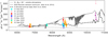 |
Fig. 3 Zenith equivalent airglow continuum radiance in the observed bandpasses according to Eq. (13). Data points are shifted by 25 Å steps to prevent them from being plotted over each other. The ESO SkyCalc yearly average residual airglow continuum (Noll et al. 2012; Jones et al. 2013), the X-shooter 2009–2019 mean airglow continuum (Noll et al. 2024), and the ZL spectrum above the atmosphere toward the ecliptic north pole (Meftah et al. (2018) solar spectrum scaled to Kelsall et al. (1998) model) are shown. Upper limits are derived in the 10 500 Å band and are indicated by arrows. |
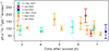 |
Fig. 4 Zenith equivalent continuum radiance as a function of time after sunset in the 6720 Å (triangles), 7700 Å (upper limits, arrows down), and 8700 Å (circles) bands. |
5.3 Temporal variability and color
In a typical case, we observed several hours after sunset. However, based on the few measurements at the beginning of the night, the airglow continuum radiance does not seem to change much over the course of the night (Fig. 4). By and large, the measured continuum seems stable and is almost flat in color, with a potential slight increase toward the red. Typically when measuring two bands during the same night, the bands measured comparable levels, with the exception being January 1, 2022, which shows a significant difference in emission between the 6720 and 8700 Å bands (see Sect. 5.4 for further discussion). The 7700 and 8700 Å bands were observed with a one-hour time difference on December 30, 2021 and March, 21 2022. On both occasions, the 7700 Å band measured equal radiance to the 8700 Å band. The 6720 and 8700 Å bands were observed with a somewhat shorter time difference on January 2, 2022, and several times on September 1, 2024. On September 1, 2024, the 8700 Å radiance remained constant within our measurement errors, with a weighted average of 126 ph s−1m−2μm−1arcsec−2, or 21.74 mag arcsec−2 and a slight tendency for the radiance to decrease toward the end of the night. The 6720 Å band has lower measurement errors and shows a statistically significant decrease over the night, with a ~40% drop in radiance between the first and last measurement. The color of the resulting continuum spectrum is flat with a marginal increase toward the red, see Fig. 3. Our data points overlap with the mean airglow spectrum of Noll et al. (2024) for Cerro Paranal, Chile.
5.4 Relation to solar activity
On January 2, 2022, the airglow continuum and OH line radiance in the 8700 Å bandpass (ID 6) measured elevated values relative to the other nights, prompting us to look for an explanation. We sought a relation to various solar activity parameters (Fig. 5). Unfortunately, the dataset is small and biased with respect to space weather: strong solar radiation activity coincided with slow solar wind conditions. No clear conclusion can be drawn, given the high temporal variability of the airglow radiance. On January 2, 2022, the 8700 Å (ID 6) measured the highest level in our data and stands out as a possible outlier in the solar activity plots (hollow marker in Fig. 5). Potentially, the increase in radiance could be due to a coronal mass ejection hitting Earth’s magnetosphere during the observation. A C1.06-class flare occurred 45 min before the beginning of the observation, and another B8.42 flare 30 min before the observation. At the beginning of the exposure, DSCOVR registered an increase in solar wind speed from an average of 525 km s−1 up to 600 km s−1, and the solar proton density increased from an average of 11 p+ cm−1 to momentarily >16 p+ cm−1, which suggests the passage of a coronal mass ejection past DSCOVR. It would have taken about 40–45 min for the particles to reach Earth’s magnetosphere, which would match the coronal mass ejection hitting right at the beginning of the observation. The 6720 Å and (ID 5) observed right after the 8700 Å measures a low continuum level but shows elevated OH 6–1 P2e,f (6.5) and 6–1 Pe,f (7.5) line emission, considering that the observation was performed more than 6.5 h after sunset.
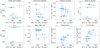 |
Fig. 5 Airglow continuum dependence in the 8700 Å bandpass on solar activity parameters, and on the OH and O2 line emissions. High solar activity coincides with slow solar wind in our dataset. Observation No 6 from January 2, 2022, with the highest measured 8700 Å radiance, is a potential outlier, as discussed in Sect. 5.4, and is indicated with a hollow symbol. The OH flux is a sum of blended 7-3 R OH lines (~8761, 8768, 8778, and 8791 Å in our spectra), while the O2 flux is a sum of blended O2 P and Q-branch lines in the range 8645–8696 Å. |
5.5 Comparison to the literature
We attempted an exhaustive literature search as part of this study to compare measurements over previous solar cycles. However, direct comparison was difficult due to differences in reporting. Few publications report the total observed continuum radiance (Broadfoot & Kendall 1968; Maihara et al. 1993b; Cuby et al. 2000; Hanuschik 2003; Sullivan & Simcoe 2012; Ellis et al. 2012; Trinh et al. 2013; Oliva et al. 2015; Nguyen et al. 2016), while others report zenith-scaled equivalents or a breakdown by components (Sternberg & Ingham 1972; Gadsden & Marovich 1973; Noxon 1978), which are ZL model- and atmospheric scattering-dependent. In some cases, exact pointing and time of observation were not reported. Allowing for these differences, the airglow continuum levels measured previously can be viewed as comparable to what we find in this work. A collections of previous airglow continuum measurements are presented in Table B.1, and units from each study were converted to those used in our work.
While the OH line emission has been studied at Observatorio del Roque de los Muchachos (Oliva et al. 2013; Franzen et al. 2018, 2019), only a single report on NIR or SWIR airglow continuum can be found in the literature (Oliva et al. 2015). Oliva et al. (2015) found comparable continuum radiance in the H band comparable to values reported for Las Campanas, Chile (Sullivan & Simcoe 2012), Cerro Paranal, Chile (Noll et al. 2024), Mauna Kea, Hawaii (Maihara et al. 1993b), and Siding Spring, Australia (Trinh et al. 2013). All VIS–NIR continuum radiance measurements were done elsewhere, most notably at Cerro Paranal, Chile Hanuschik (2003); Noll et al. (2024). We compare our results to measurements made at other sites below.
Hanuschik (2003) observed apparent continuum radiance of 300–350 ph s−1m−2μm−1arcsec−2 in the wavelength range observed in this work. Exact dates of observations are not reported, but the reported Moon illumination fraction restricts the dates to 20–21 June 2001. Hanuschik (2003) observed at a mean air mass of z = 1.11, forcing the pointings quite close to the ecliptic equator, with a maximum distance of approximately βec ~ −33°. The Kelsall et al. (1998) model gives an ~100 ph s−1m−2μm−1arcsec−2 ZL contribution to the total apparent continuum. The Hanuschik (2003) spectra appear bluer than that which we find in this work, but the level is comparable after accounting for ZL on the nights associated with stronger solar activity in our study. On 20–21 June 2001, DRAO F10.7 ranged between 199–204 sfu, indicating moderately high solar activity.
Sternberg & Ingham (1972) reported a time series of ZL corrected observations at 8200 Å toward the North Celestial Pole from the Haute-Provence observatory, during nights of August 18 to 19, 1969 with a nightly decrease from 300 to 190 ph s−1m−2μm−1arcsec−2. Kelsall et al. (1998) reported a ZL radiance for their pointing of ~40 ph s−1m−2μm−1arcsec−2. The level is similar to that found by Hanuschik (2003). The decay resembles behavior observed in this work on 1 September 2024. Sternberg & Ingham (1972) observed bad weather, potentially affecting the observations, without elaborating further. Sternberg & Ingham (1972) found a close to constant continuum emission of 75 ph s−1m−2μm−1arcsec−2 at 6750 Å on 2 June 1970.
The ESO Sky Calc (Noll et al. 2012; Jones et al. 2013; Noll et al. 2013) residual airglow continuum offers another point of comparison. The residual airglow continuum model is based on 26 averaged early X-shooter spectra. The Noll et al. (2012) residual continuum showed a significant increase toward red between 7000 and 9000 Å, which resembles the behavior reported by Broadfoot & Kendall (1968). Similar reddening was also reported by Gadsden & Marovich (1973). Noxon (1978) did not observe an increase in radiance and suggested that the reddening reported by Gadsden & Marovich (1973) and Broadfoot & Kendall (1968) may have been instrumental. More recently, Noll et al. (2024) attributes the increase toward longer wavelengths in the Noll et al. (2012) study to the low resolution of the FOcal Reducer and low dispersion Spectrograph 1 (FORS 1) used in that study. Nonetheless, we may have witnessed similar reddening associated with stronger solar activity on the night of September 1, 2024. Noll et al. (2024) finds a much flatter airglow continuum spectrum based on a larger X-shooter dataset covering late 2009 to 2019. The flat continuum spectrum is similar to what we observed at Roque de los Muchachos.
5.6 Implications
Our observations indicate a dark interline NIR sky. To take full advantage of it for faint object spectroscopy, its properties should be investigated further. Our work may also encourage the introduction of OH line suppressors and grating-stray-light-reducing spectrograph designs to workhorse NIR and SWIR spectrographs. Successful OH line suppressors based on line masks (e.g., Maihara et al. 1993a; Iwamuro et al. 2001; Parry et al. 2004) and Fiber Bragg Gratings (e.g., Ellis et al. 2012) have been demonstrated in the literature. The grating-scattering-wing-reducing spectrograph designs use the grating in a double-pass configuration combined with a secondary slit between the dispersions. The double-pass spectrograph can be implemented either as a scanning monochromator (Enard 1982) (compatible with long slits, but records only a single spectral element at a time), or as a white-pupil spectrograph with a beam rotation between the two dispersions (Andersen & Andersen 1992; Viuho et al. 2022) (confined to use with round apertures, i.e., fibers, with the advantage of recording the full spectral range at once).
We observed variations of up to a factor of two in the VIS–NIR airglow continuum on timescales from tens of minutes to hours. Our observations do not temporally resolve the shorter timescale variations associated with mesospheric buoyancy waves, and it is possible that the airglow continuum exhibits variation similar to those of the airglow line emission on minute timescales. We do not have data to study the seasonal variability reported by Patat (2008) and Noll et al. (2024), and it is difficult to secure observing time for a nonstandard optical configuration for a long-term monitoring program. Temporal variability of the continuum radiance needs to be taken into account when designing faint object spectrographs for ground-based observations, even when OH suppressing or double-pass techniques are being used.
6 Conclusion
We measured the NIR airglow continuum radiance at the Observatorio del Roque de los Muchachos with control over the instrumental line wing contribution. We find the continuum radiance to range between 60–170 ph s−1m−2μm−1arcsec−2, or 21.4–22.8 mag arcsec−2, depending on the bandpass and the time of observation. The zenith-scaled airglow continuum radiance is two to four times brighter than the ZL toward the ecliptic poles: the darkest foreground available for ground- and current space-based observatories. The observations carried out under photometric observing conditions establish a solid measurement for the darkest sky conditions. We observe the continuum to be stable with a modest decay toward the end of the night. The observations presented here were sporadically spread across the year, and we are unable to study the seasonal variability reported in the literature. We promote a long-term observing campaign for its analysis. Our work demonstrates that the VIS-NIR sky continuum can be very dark under photometric conditions, offering close to ZL-limited foreground from the ground in the NIR sensitivity range of silicon photodetectors, encouraging the design of astronomical spectrographs taking advantage of the dark interline sky.
Data availability
Raw data are available on the NOT’s fits archive, or upon request from the corresponding author. Scripts used as part of the work are available upon reasonable request from the corresponding author.
Acknowledgements
The Cosmic Dawn Center (DAWN) is funded by the Danish National Research Foundation under grant DNRF140. The data presented here were obtained in part with ALFOSC, which is provided by the Instituto de Astrofisica de Andalucia (IAA) under a joint agreement with the University of Copenhagen and NOT. The COBE datasets were developed by NASA’s Goddard Space Flight Center under the guidance of the COBE Science Working Group and were provided by the NSSDC. DSCOVR and GOES data courtesy to National Oceanic (NOAO) and Atmospheric Administration Space Weather Prediction Center (SWPC). F10.7 data courtesy to the DRAO. We thank J. Munday, V. Pinter, A. E. T. Viitanen, and A. N. Sørensen for discussion and their valuable feedback on the manuscript.
Appendix A Observed apparent continuum spectra
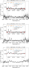 |
Fig. A.1 Apparent airglow spectra observed in 6720 Å band. The 2022 spectra were recorded with a 0.5″ slit whereas, the 2024 spectra are recorded with a 1.3″ slit. Spectral lines found in Hanuschik (2003) are indicated with blue ticks, with the tick length indicating relative intensity. Locations of computed OH lines by van der Loo & Groenenboom (2007, 2008) are shown with orange ticks, with the tick length indicating the line’s Einstein coefficient. The noise floor is shown as a dashed gray line, and the spectral regions used for sampling the continuum are indicated in red. |
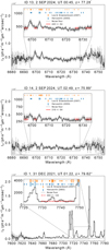 |
Fig. A.2 6720 Å band spectra continued, along with apparent airglow radiance in the 7700 Å band. No clean spectral region is found without known lines or atmospheric absorption features. An upper limit on the continuum radiance is derived from regions free from O2 absorption, which nonetheless contain unresolved spectral lines. |
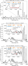 |
Fig. A.3 7700 Å band airglow spectra continued. Apparent airglow spectra are shown in the 8700Å band. |
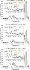 |
Fig. A.4 Apparent airglow spectra in 8700Å band continued. |
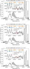 |
Fig. A.5 Apparent airglow spectra in the 8700Å band continued. |
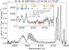 |
Fig. A.6 Apparent airglow spectra in the 8700Å band continued. |
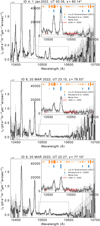 |
Fig. A.7 Apparent airglow spectra in the 10 500 Å band. Due to low system efficiency, the continuum in 10 500 Å is indistinguishable from the detector noise in all our spectra. |
Appendix B Previous studies and solar data
Compilation of NIR and SWIR airglow continuum measurements in the literature.
Space weather conditions at the time of observation.
References
- Andersen, M. I., & Andersen, J. 1992, in ESO Workshop on High Resolution Spectroscopy with the VLT, 40 (European Southern Observatory), 235 [Google Scholar]
- Arendt, R. G., Odegard, N., Weiland, J. L., et al. 1998, ApJ, 508, 74 [NASA ADS] [CrossRef] [Google Scholar]
- Baker, D. J., & Stair, A. T. 1988, Phys. Scr., 37, 611 [Google Scholar]
- Bates, D. R. 1993, Proc. Roy. Soc. Lond. Ser. A: Math. Phys. Sci., 443, 227 [Google Scholar]
- Broadfoot, A. L., & Kendall, K. R. 1968, J. Geophys. Res., 73, 426 [Google Scholar]
- Colina, L., & Bohlin, R. C. 1994, AJ, 108, 1931 [Google Scholar]
- Cuby, J. G., Lidman, C., & Moutou, C. 2000, The Messenger, 101, 2 [Google Scholar]
- Dwek, E., Arendt, R. G., Hauser, M. G., et al. 1998, ApJ, 508, 106 [NASA ADS] [CrossRef] [Google Scholar]
- Ellis, S. C., & Bland-Hawthorn, J. 2008, MNRAS, 386, 47 [Google Scholar]
- Ellis, S. C., Bland-Hawthorn, J., Lawrence, J., et al. 2012, MNRAS, 425, 1682 [Google Scholar]
- Ellis, S. C., Bland-Hawthorn, J., Lawrence, J. S., et al. 2020, MNRAS, 492, 2796 [Google Scholar]
- Enard, D. 1982, SPIE Conf. Ser., 331, 232 [NASA ADS] [Google Scholar]
- Flewelling, H. A., Magnier, E. A., Chambers, K. C., et al. 2020, ApJS, 251, 7 [NASA ADS] [CrossRef] [Google Scholar]
- Franzen, C., Espy, P. J., Hibbins, R. E., & Djupvik, A. A. 2018, J. Geophys. Res.: Atmos., 123, 10935 [Google Scholar]
- Franzen, C., Espy, P. J., Hofmann, N., Hibbins, R. E., & Djupvik, A. A. 2019, Atmosphere, 10, 637 [Google Scholar]
- Gadsden, M., & Marovich, E. 1973, J. Atmos. Terrestr. Phys., 35, 1601 [Google Scholar]
- Giavalisco, M., Ferguson, H. C., Koekemoer, A. M., et al. 2004, ApJ, 600, L93 [NASA ADS] [CrossRef] [Google Scholar]
- Gorjian, V., Wright, E. L., & Chary, R. R. 2000, ApJ, 536, 550 [Google Scholar]
- Grygalashvyly, M., Pogoreltsev, A. I., Andreyev, A. B., Smyshlyaev, S. P., & Sonnemann, G. R. 2021, Ann. Geophys., 39, 255 [Google Scholar]
- Hanuschik, R. W. 2003, A&A, 407, 1157 [NASA ADS] [CrossRef] [EDP Sciences] [Google Scholar]
- Hauser, M. G., Arendt, R. G., Kelsall, T., et al. 1998, ApJ, 508, 25 [Google Scholar]
- Iwamuro, F., Motohara, K., Maihara, T., Hata, R., & Harashima, T. 2001, PASJ, 53, 355 [NASA ADS] [Google Scholar]
- Jones, A., Noll, S., Kausch, W., Szyszka, C., & Kimeswenger, S. 2013, A&A, 560, A91 [NASA ADS] [CrossRef] [EDP Sciences] [Google Scholar]
- Kawara, K., Matsuoka, Y., Sano, K., et al. 2017, PASJ, 69, 31 [NASA ADS] [CrossRef] [Google Scholar]
- Kelsall, T., Weiland, J. L., Franz, B. A., et al. 1998, ApJ, 508, 44 [Google Scholar]
- Khomich, V. Y., Semenov, A. I., & Shefov, N. N. 2008, Airglow as an Indicator of Upper Atmospheric Structure and Dynamics, 1st edn. (Berlin, Heidelberg: Springer-Verlag) [Google Scholar]
- King, D. L. 1985, Atmospheric Extinction at the Roque de los Muchachos Observatory, La Palma, RGO/La Palma technical note no 31 [Google Scholar]
- Koch, F., Zilk, M., & Glaser, T. 2021, Proc. SPIE, 11783, 1178304 [Google Scholar]
- Kramida, A., Yu. Ralchenko, Reader, J., & NIST ASD Team 2023, NIST Atomic Spectra Database (ver. 5.11), [Online]. Available: https://physics.nist.gov/asd [2024, October 15]. National Institute of Standards and Technology, Gaithersburg, MD [Google Scholar]
- Krassovsky, V. I., Shefov, N. N., & Yarin, V. I. 1962, Planet. Space Sci., 9, 883 [Google Scholar]
- Krisciunas, K. 1997, PASP, 109, 1181 [Google Scholar]
- Krisciunas, K., & Schaefer, B. E. 1991, PASP, 103, 1033 [Google Scholar]
- Leinert, C., Väisänen, P., Mattila, K., & Lehtinen, K. 1995, A&AS, 112, 99 [Google Scholar]
- Leinert, C., Bowyer, S., Haikala, L. K., et al. 1998, A&AS, 127, 1 [NASA ADS] [CrossRef] [EDP Sciences] [Google Scholar]
- Levasseur-Regourd, A. C., & Dumont, R. 1980, A&A, 84, 277 [NASA ADS] [Google Scholar]
- Liou, K.-N. 2002, An Introduction to Atmospheric Radiation, 2nd edn., International Geophysics Series, 84 (San Diego, Calif.: Academic Press) [Google Scholar]
- Lopez-Moreno, J. J., Rodrigo, R., Moreno, F., Lopez-Puetas, M., & Molina, A. 1987, Planet. Space Sci., 35, 1029 [Google Scholar]
- Maihara, T., Iwamuro, F., Hall, D. N. B., et al. 1993a, in Infrared Detectors and Instrumentation, 1946 (International Society for Optics and Photonics), 581 [Google Scholar]
- Maihara, T., Iwamuro, F., Yamashita, T., et al. 1993b, PASP, 105, 940 [Google Scholar]
- Mattila, K., Väisänen, P., & Appen-Schnur, G. F. O. V. 1996, A&AS, 119, 153 [NASA ADS] [CrossRef] [EDP Sciences] [Google Scholar]
- Meftah, M., Damé, L., Bolsée, D., et al. 2018, A&A, 611, A1 [NASA ADS] [CrossRef] [EDP Sciences] [Google Scholar]
- Moreels, G., Clairemidi, J., Faivre, M., et al. 2008, Exp. Astron., 22, 87 [Google Scholar]
- Murdin, P. 1986, Geology and meteorology of Saharan dust, RGO/La Palma technical note no. 41 [Google Scholar]
- Nguyen, H. T., Zemcov, M., Battle, J., et al. 2016, PASP, 128, 094504 [Google Scholar]
- Noll, S., Kausch, W., Barden, M., et al. 2012, A&A, 543, A92 [NASA ADS] [CrossRef] [EDP Sciences] [Google Scholar]
- Noll, S., Kausch, W., Barden, M., et al. 2013, The Cerro Paranal Advanced Sky Model, VLT-MAN-ESO-19550-5339 [Google Scholar]
- Noll, S., Kimeswenger, S., Proxauf, B., et al. 2017, J. Atmos. Sol. Terrestr. Phys., 163, 54 [Google Scholar]
- Noll, S., Plane, J. M. C., Feng, W., et al. 2024, Atmos. Chem. Phys., 24, 1143 [Google Scholar]
- Noll, S., Schmidt, C., Hannawald, P., Kausch, W., & Kimeswenger, S. 2025, EGUsphere, 2025, 1 [Google Scholar]
- Noxon, J. F. 1978, Planet. Space Sci., 26, 191 [Google Scholar]
- Oke, J. B. 1974, ApJS, 27, 21 [Google Scholar]
- Oliva, E., Origlia, L., Maiolino, R., et al. 2013, A&A, 555, A78 [NASA ADS] [CrossRef] [EDP Sciences] [Google Scholar]
- Oliva, E., Origlia, L., Scuderi, S., et al. 2015, A&A, 581, A47 [NASA ADS] [CrossRef] [EDP Sciences] [Google Scholar]
- Osterbrock, D. E., Fulbright, J. P., Martel, A. R., et al. 1996, PASP, 108, 277 [Google Scholar]
- Parry, I., Bunker, A., Dean, A., et al. 2004, in Ground-based Instrumentation for Astronomy, 5492, eds. A. F. M. Moorwood, & M. Iye [Google Scholar]
- Patat, F. 2008, A&A, 481, 575 [NASA ADS] [CrossRef] [EDP Sciences] [Google Scholar]
- Pickles, A. J. 1998, PASP, 110, 863 [NASA ADS] [CrossRef] [Google Scholar]
- Plane, J. M., Feng, W., & Dawkins, E. C. 2015, Chem. Rev., 115, 4497 [Google Scholar]
- Rousselot, P., Lidman, C., Cuby, J.-G., liu, G., & Monnet, G. 2000, A&A, 354, 1134 [Google Scholar]
- Rubin, D., Aldering, G., Antilogus, P., et al. 2022, ApJS, 263, 1 [NASA ADS] [CrossRef] [Google Scholar]
- Scoville, N., Abraham, R., Aussel, H., et al. 2007, ApJS, 172, 38 [NASA ADS] [CrossRef] [Google Scholar]
- Smith, A. K. 2012, Surv. Geophys., 33, 1177 [Google Scholar]
- Smith, S. M., Scheer, J., Reisin, E. R., Baumgardner, J., & Mendillo, M. 2006, J. Geophys. Res.: Space Phys., 111, A09309 [Google Scholar]
- Sobolev, V. G. 1978, Planet. Space Sci., 26, 703 [Google Scholar]
- Sternberg, J. R., & Ingham, M. F. 1972, MNRAS, 159, 1 [NASA ADS] [Google Scholar]
- Sullivan, P. W., & Simcoe, R. A. 2012, PASP, 124, 1336 [Google Scholar]
- Tapping, K. F. 2013, Space Weather, 11, 394 [CrossRef] [Google Scholar]
- Tilvi, V., Rhoads, J. E., Hibon, P., et al. 2010, ApJ, 721, 1853 [Google Scholar]
- Tody, D. 1986, SPIE Conf. Ser., 627, 733 [Google Scholar]
- Tody, D. 1993, in Astronomical Society of the Pacific Conference Series, 52, Astronomical Data Analysis Software and Systems II, eds. R. J. Hanisch, R. J. V. Brissenden, & J. Barnes, 173 [Google Scholar]
- Trinh, C. Q., Ellis, S. C., Bland-Hawthorn, J., et al. 2013, MNRAS, 432, 3262 [Google Scholar]
- Tsumura, K., Matsumoto, T., Matsuura, S., et al. 2013, PASJ, 65, 119 [Google Scholar]
- van der Loo, M. P. J., & Groenenboom, G. C. 2007, J. Chem. Phys., 126, 114314 [Google Scholar]
- van der Loo, M. P. J., & Groenenboom, G. C. 2008, J. Chem. Phys., 128, 159902 [Google Scholar]
- van Dokkum, P. G. 2001, PASP, 113, 1420 [Google Scholar]
- van Rhijn, P. J. 1921, Publications of the Astronomical Laboratory at Groningen, 31, 1 [Google Scholar]
- Venemans, B. P., McMahon, R. G., Parry, I. R., et al. 2009, in Astrophysics and Space Science Proceedings, 9, Science with the VLT in the ELT Era, 187 [Google Scholar]
- Verro, K., Trager, S. C., Peletier, R. F., et al. 2022, A&A, 660, A34 [NASA ADS] [CrossRef] [EDP Sciences] [Google Scholar]
- Viuho, J. K. M., Andersen, M. I., & U., F. J. P. 2022, in Ground-based and Airborne Instrumentation for Astronomy IX, 12184, eds. C. J. Evans, J. J. Bryant, & K. Motohara, International Society for Optics and Photonics (SPIE), 1218456 [Google Scholar]
- Weaver, J. R., Kauffmann, O. B., Ilbert, O., et al. 2022, ApJS, 258, 11 [NASA ADS] [CrossRef] [Google Scholar]
- Williams, R. E., Blacker, B., Dickinson, M., et al. 1996, AJ, 112, 1335 [NASA ADS] [CrossRef] [Google Scholar]
- Windhorst, R. A., Carleton, T., O’Brien, R., et al. 2022, AJ, 164, 141 [NASA ADS] [CrossRef] [Google Scholar]
- Woods, T. N., Wrigley, R. T., Rottman, G. J., & Haring, R. E. 1994, Appl. Opt., 33, 4273 [Google Scholar]
- Wright, E. L. 1998, ApJ, 496, 1 [NASA ADS] [CrossRef] [Google Scholar]
We define the spectral ranges referred to often in the following way: visible 4000–7000 Å (VIS), near-infrared (NIR) 7000–11 000 Å, and short-wave infrared (SWIR) 1.1–3 μm. All magnitudes in our work refer to those in the AB system.
All Tables
All Figures
|
Fig. 1 Projection of the COBE/DIRBE band 1 map with a central wavelength at 1.25 μm toward the ecliptic north pole. The red markers indicate the coordinates for our pointings, the HDF, and the COSMOS field. The Milky Way crosses the map horizontally, while ZL in the ecliptic plane appears as a ring between declinations δ = [−30, 30]. |
| In the text | |
|
Fig. 2 Transmission curves of the NB filters, order-sorting broad-band filters, grism blaze functions, detector efficiency, and atmospheric transmission at the observed zenith distance. The blue half of the 7700 Å band is strongly absorbed by atmospheric O2. In the 10 500 Å band, the total system efficiency is very low, as the wavelength falls within the wing of the grism blaze function. |
| In the text | |
|
Fig. 3 Zenith equivalent airglow continuum radiance in the observed bandpasses according to Eq. (13). Data points are shifted by 25 Å steps to prevent them from being plotted over each other. The ESO SkyCalc yearly average residual airglow continuum (Noll et al. 2012; Jones et al. 2013), the X-shooter 2009–2019 mean airglow continuum (Noll et al. 2024), and the ZL spectrum above the atmosphere toward the ecliptic north pole (Meftah et al. (2018) solar spectrum scaled to Kelsall et al. (1998) model) are shown. Upper limits are derived in the 10 500 Å band and are indicated by arrows. |
| In the text | |
|
Fig. 4 Zenith equivalent continuum radiance as a function of time after sunset in the 6720 Å (triangles), 7700 Å (upper limits, arrows down), and 8700 Å (circles) bands. |
| In the text | |
|
Fig. 5 Airglow continuum dependence in the 8700 Å bandpass on solar activity parameters, and on the OH and O2 line emissions. High solar activity coincides with slow solar wind in our dataset. Observation No 6 from January 2, 2022, with the highest measured 8700 Å radiance, is a potential outlier, as discussed in Sect. 5.4, and is indicated with a hollow symbol. The OH flux is a sum of blended 7-3 R OH lines (~8761, 8768, 8778, and 8791 Å in our spectra), while the O2 flux is a sum of blended O2 P and Q-branch lines in the range 8645–8696 Å. |
| In the text | |
|
Fig. A.1 Apparent airglow spectra observed in 6720 Å band. The 2022 spectra were recorded with a 0.5″ slit whereas, the 2024 spectra are recorded with a 1.3″ slit. Spectral lines found in Hanuschik (2003) are indicated with blue ticks, with the tick length indicating relative intensity. Locations of computed OH lines by van der Loo & Groenenboom (2007, 2008) are shown with orange ticks, with the tick length indicating the line’s Einstein coefficient. The noise floor is shown as a dashed gray line, and the spectral regions used for sampling the continuum are indicated in red. |
| In the text | |
|
Fig. A.2 6720 Å band spectra continued, along with apparent airglow radiance in the 7700 Å band. No clean spectral region is found without known lines or atmospheric absorption features. An upper limit on the continuum radiance is derived from regions free from O2 absorption, which nonetheless contain unresolved spectral lines. |
| In the text | |
|
Fig. A.3 7700 Å band airglow spectra continued. Apparent airglow spectra are shown in the 8700Å band. |
| In the text | |
|
Fig. A.4 Apparent airglow spectra in 8700Å band continued. |
| In the text | |
|
Fig. A.5 Apparent airglow spectra in the 8700Å band continued. |
| In the text | |
|
Fig. A.6 Apparent airglow spectra in the 8700Å band continued. |
| In the text | |
|
Fig. A.7 Apparent airglow spectra in the 10 500 Å band. Due to low system efficiency, the continuum in 10 500 Å is indistinguishable from the detector noise in all our spectra. |
| In the text | |
Current usage metrics show cumulative count of Article Views (full-text article views including HTML views, PDF and ePub downloads, according to the available data) and Abstracts Views on Vision4Press platform.
Data correspond to usage on the plateform after 2015. The current usage metrics is available 48-96 hours after online publication and is updated daily on week days.
Initial download of the metrics may take a while.