| Issue |
A&A
Volume 698, May 2025
|
|
|---|---|---|
| Article Number | A212 | |
| Number of page(s) | 11 | |
| Section | Astronomical instrumentation | |
| DOI | https://doi.org/10.1051/0004-6361/202554532 | |
| Published online | 20 June 2025 | |
Advanced modelling of the night sky background light for imaging atmospheric Cherenkov telescopes
1
Friedrich-Alexander-Universität Erlangen-Nürnberg, Erlangen Centre for Astroparticle Physics,
Nikolaus-Fiebiger-Str. 2,
91058
Erlangen,
Germany
2
Department of Physics, Clarendon Laboratory,
Parks Road,
Oxford
OX1 3PU,
UK
★ Corresponding author: gerrit.roellinghoff@fau.de
Received:
14
March
2025
Accepted:
15
May
2025
Aims. A significant source of noise for imaging atmospheric Cherenkov telescopes (IACTs), which are designed to measure air showers caused by astrophysical gamma rays, is optical light emitted from the night sky. This night sky background (NSB) influences IACT operating times and their sensitivity. Thus, for scheduling observations and instrument simulation, an accurate estimate of the NSB is important.
Methods. A physics-driven approach to simulating wavelength-dependent, per-photomultiplier-pixel NSB was developed. It included contributions from scattered moonlight, starlight, diffuse galactic light, zodiacal light, and airglow emission. It also accounted for the absorption and scattering of optical light in the atmosphere and telescope-specific factors such as mirror reflectivity, photon detection efficiency, and focal length. The simulated results were corrected for pointing inaccuracies and individual pixel sensitivities and were compared to data from the high energy stereoscopic system (H.E.S.S.) IACT array. The software package developed for this analysis will be made publicly available.
Results. Validation against H.E.S.S. data shows small deviations from the prediction, which are attributable to airglow and atmospheric variability. Per-pixel predictions provide a good match to the data, with a relative 90% error range of [‒21%, 19%]. Compared to the existing standard modelling approach of assuming a constant background, which yields a relative 90% error range of [−64%, 48%], this represents a significant improvement.
Key words: astroparticle physics / atmospheric effects / instrumentation: detectors / methods: data analysis / gamma rays: general
© The Authors 2025
 Open Access article, published by EDP Sciences, under the terms of the Creative Commons Attribution License (https://creativecommons.org/licenses/by/4.0), which permits unrestricted use, distribution, and reproduction in any medium, provided the original work is properly cited.
This article is published in open access under the Subscribe to Open model. Subscribe to A&A to support open access publication.
1 Introduction
Imaging atmospheric Cherenkov telescopes (IACTs) are indirect detection instruments for the observation of very-high-energy gamma rays (>20GeV). These gamma rays induce particle air showers in the Earth’s atmosphere, whose charged component particles cause the emission of Cherenkov light due to their superluminal passage through air. IACTs observe this light by using large mirror arrays to focus it on the focal plane of highspeed cameras, whose pixels consist of photomultiplier tubes (PMTs) or silicon photomultipliers (SiPMs). If a sufficient number of pixels within a time window detect light reminiscent of the shape expected for an air shower, a trigger logic is activated, and all the pixel values are read out. The time resolution of IACTs is typically of the order of a few nanoseconds, compared to the arrival time frame of air shower photons of about 10 ns (Ashton et al. 2020). This allows for the detection of the faint amount of photons from air showers, which would generally be overshadowed by other sources of photons in the night sky.
The high energy stereoscopic system (H.E.S.S.) detector array, stationed 1800 m above sea level, consists of two different types of IACTs: an initial four telescopes arranged in a square (CT1-4, construction finished in 2004), each with about 107 m2 mirror area, and a central single dish with about 600 m2 mirror area (CT5, constructed in 2012). The original cameras for CT1- 4 were upgraded between 2015 and 2017 with NECTAr-based electronics (Giavitto et al. 2017; Ashton et al. 2020). The CT5 camera was changed in 2019 to a camera following the FlashCam design developed for future use in the medium-sized telescopes of the Cherenkov telescope array observatory (CTAO) (Werner et al. 2017; Puehlhofer et al. 2022; Bi et al. 2022). Table 1 shows the properties of CT1-4. The readout of a single pixel is always defined in relation to a pedestal value. This pixel pedestal value depends on the electronic readout noise, gain, and the illumination level of the pixel from constant light sources, with a higher constant illumination leading to a wider distribution of pedestal values.
Exposure to the night sky results in IACT images containing additional light called night sky background (NSB). Major contributions to NSB are airglow in the upper atmosphere, scattered moonlight, zodiacal light, and starlight. Other factors, such as the diffuse galactic light (DGL), light pollution, and ground reflections, have minor contributions at dark sites. The NSB also heavily depends on atmospheric conditions, which in turn depend on telescope location, time of observation, and pointing direction. Both the scattering and the absorption of light are dependent on local atmospheric conditions such as aerosol concentration, aerosol albedo, humidity, and temperature (Garstang 1991; Leinert et al. 1998; Noll et al. 2012).
For valid computational reasons, NSB modelling to date for IACTs has been limited. While there are tools to utilise NSB maps and model starlight in IACTs (Bernlöhr 2008; Büchele 2020), the common approach is to use an NSB spectrum taken from the night sky over La Palma by Benn & Ellison (1998) (Bernlöhr 2008). The NSB is then scaled based on the expected rate and applied to the entire telescope, with the expected rate being informed by past observations. As such, the NSB is implicitly considered homogeneous over the field of view (FoV) of the telescope in these cases. However, some areas of the sky observed by IACTs have very inhomogeneous NSB (see Sect. 3.3). Improved NSB modelling has a wide variety of applications for IACTs, which we discuss in Sect. 4.2.
With the inclusion of observations under moonlight conditions in the schedules of major IACTs (Griffin & VERITAS Collaboration 2015; Ahnen et al. 2017; Tomankova et al. 2022), reliable NSB predictions have become more important, since some observation positions are rendered impossible due to their proximity to the Moon (as overexposing PMTs can lead to damage). In the H.E.S.S. collaboration, the expected NSB contribution of the Moon was included in the auto-scheduler (2020, priv. commun.), using an adjusted model from Krisciunas & Schaefer (1991) fitted to the photometric data of the sky obtained from Mauna Kea and two sites in Russia in the 1990s. While this includes an estimate for the moonlight and airglow contributions to NSB, it neither deals with the inhomogeneity of NSB over the field of view, nor the addition of other NSB sources such as starlight. This can lead to the underestimation of the expected NSB, since starlight-bright regions of the sky (especially our own Galaxy) can be comparable to the contribution of moonlight, depending on the separation angle from the Moon. A previous study by Spencer et al. (2024) on per-pixel NSB in the small size telescopes (SSTs) for CTAO included the contribution of starlight, adding the V-band photometric data from the Hipparcos/Tycho and Gaia catalogues to the NSB model from Krisciunas & Schaefer (1991). For this, it uses a modified version of the nsb1 package developed by Büchele (2020) and colleagues for use by the H.E.S.S. collaboration. To the best of our knowledge, there have been no studies comparing simulated NSB to actual NSB values on a per-pixel level in the realm of IACTs to date.
In IACT event reconstruction, gamma-ray air shower parameters are extracted from pedestal-subtracted pixel values. As elevated NSB values increase the pedestal distribution width, it statistically smears out the signal values in each pixel. While this does not introduce energy bias, it worsens energy resolution and the gamma-ray point spread function (PSF) of the instrument. It can also have an effect on the effective area of the instrument, which, depending on the analysis, can have a larger effect (Holler et al. 2020). This effect is unique to each NSB pattern and cannot be simulated using homogeneous NSB. IACT arrays currently take observations in so-called ‘runs’ targeting a particular position on the sky, over which observing conditions are assumed to be approximately constant. For H.E.S.S., runs can be up to 28 minutes in duration. Computing approaches such as run-wise simulation incorporate the effect of distinct NSB patterns for each run on event reconstruction, relying on per-pixel NSB values calculated from data. This approach has been shown to match the data well (Holler et al. 2020).
The NSB and its contributing factors have been extensively studied outside of gamma ray astronomy (for example, see Benn & Ellison (1998) for La Palma or Patat (2008) for Cerro Paranal). Leinert et al. (1998) gives an overview of the measurements and models for the different contributions to the NSB, ranging from ultraviolet to infrared wavelengths. It includes airglow, zodiacal light, diffuse galactic and extragalactic light, and integrated starlight. Noll et al. (2012) introduced and validated an extensive spectrographic model for the NSB at Cerro Paranal in optical and infrared wavelengths. It includes a detailed discussion about atmospheric absorption and scattering, and was updated with an improved model of lunar contribution by Jones et al. (2013). In a similar vein, Masana et al. (2021) created GAMBONS, which models the NSB over the sky hemisphere for the purpose of light pollution measurements. Transferring some of the techniques and measurements from other areas of astronomy is, therefore, an obvious way to improve NSB modelling for IACTs.
The remainder of this work is structured as follows: in Sect. 2, we introduce a new, physically motivated model for the prediction of NSB in IACTs and its components. In Sect. 3, we describe the application of this model to the H.E.S.S. telescopes and evaluate its accuracy using actual NSB data covering one year of observations. In Sect. 4, we discuss the validity of the approach, systematics, and possible areas of application. Lastly, in Sect. 5, we summarise our findings, discuss their implications for further IACT research, and outline further possible areas of improvement for modelling NSB in IACT observations.
Telescope parameters for the H.E.S.S. I telescopes.
2 Methods
In general, NSB can be described as the sum of all contributing radiances at an observer location x detected in direction ω at a specific wavelength λ:
 (1)
(1)
This can be separated into the out-of-atmosphere radiance of  (λ, ω) and the atmospheric propagation term T(λ, ω, x). The atmospheric propagation term can be further separated into:
Atmospheric attenuation Ta(λ, ω, x), with light in the line of sight (LoS) being scattered out of the LoS or absorbed by the atmosphere.
Atmospheric enhancement Ts(λ, ω, ωs, x) due to inscattering, where light from a position ωs outside the LoS gets scattered into the LoS.
With this, we can write the expected NSB over all sources i of radiance as
 (2)
(2)
Lastly, the photon flux Ф(ω, x) depends on the bandpass S (λ) of the instrument measuring the NSB:
 (3)
(3)
For diffuse sources, the integral in the second term is often approximated as a modification to the attenuation term (Kwon et al. 2004; Kocifaj 2009; Noll et al. 2012; Winkler 2022), resulting in an effective atmospheric transmittance Teff(λ, ω, x):
 (4)
(4)
In general, the above equations also depend on the time t, especially in the context of coordinate transforms. To transform to source-dependent reference frames, we needed to know the transformation from local coordinates (ω, x) to galactic (l, b), equatorial (α, δ), or heliocentric ecliptic (ʌ, β) coordinates. For this, we used the AstroPy2 software package (Astropy Collaboration 2013, 2018, 2022).
To calculate the photon rate for a single pixel in a telescope, the local coordinates (ω, x) need to be transformed to telescope coordinates (x, y) depending on the direction η the telescope is pointing. The total rate Fsim for pixel j is then equivalent to
 (5)
(5)
where P(x, y|ω) is the telescope point source function, Aj is the pixel area, and η is the telescope pointing direction. Computationally, this can be approximated as
 (6)
(6)
where wx,y, is the weight assigned to the position (x,y) on the pixel for the corresponding discrete integration scheme and Cj(η) is the set of positions in the sky with significant contribution to the rate in pixel j.
2.1 Sources of NSB
2.1.1 Moonlight
In the context of NSB, the most significant source in the night sky is the Moon. During the brightest lunar phase of full moon, with an average visual magnitude of −12.7, its radiative flux is about 2000 times higher than that of the second brightest object (Venus). As such, as long as the Moon is above the horizon and its phase angle is small (Table 2, Krisciunas & Schaefer 1991), moonlight is the dominating contribution to the NSB at most positions on the sky.
Krisciunas & Schaefer (1991) used an empirical fit of the scattering function to data from Mauna Kea and two Russian sites and an empirical function modifying the moon brightness based on lunar phase to create a formula for the expected lunar contribution in the V band. Being one of the first formulas for moonlight brightness, they achieved an rms uncertainty for the V band of 23%. Jones et al. (2013) improved on this concept by incorporating an accurate solar spectrum, a lunar albedo fit to the data by Kieffer & Stone (2005), and a physically based atmospheric model. They reached an uncertainty of less than 20% over the optical range when comparing their spectra to measured FORS1 spectra. Winkler (2022) modified their approach, differing in the use of an analytical treatment of atmospheric scattering and their interpolation of lunar albedo values. When fitting the offset, their resulting uncertainty is typically of the order of less than 5% in the UBVRI bands. For the light emission component of the moonlight, we followed Jones et al. (2013), with our atmospheric scattering approach described in Sect. 2.2.
The intensity Ilun of moonlight entering the Earth’s atmosphere following Jones et al. (2013) is related to the solar light intensity Iʘ via
 (7)
(7)
where ΩM is the solid angle of the Moon (ΩM = 6.4177 x 10⁻⁵ sr) and DM is the distance to Earth. The solar spectrum is taken from Rieke et al. (2008). The lunar Albedo A is a wavelength-dependent fit to the observational data performed by Kieffer & Stone (2005):
![\begin{aligned} ln(A(\lambda)) = & \sum_{i=0}^3 a_{i,\lambda}g^i + \sum_{j=1}^3 b_{j,\lambda}\Phi^{2j-1} \\& + d_{1,\lambda}e^{-g/p_1} + d_{2,\lambda}e^{-g/p_2} + d_{3,\lambda}\cos[(g-p_3)/2], \end{aligned}](/articles/aa/full_html/2025/06/aa54532-25/aa54532-25-eq9.png) (8)
(8)
where g is the lunar phase parameter and Ф is the solar selenographic longitude. The values for pn, ah, bj, dn are taken from Kieffer & Stone (2005). Then a quadratic spline is fitted to determine Ilun (λ) in a smooth manner. For our purposes, the Moon is assumed to be a point source due to the fact that H.E.S.S. observations are separated by at least 10° from the Moon.
2.1.2 Zodiacal light
Zodiacal light is caused by solar light reflected off interplanetary dust grains in the ecliptic. As such, it is highly dependent on the ecliptic coordinates, with the NSB rate decreasing with increasing ecliptic latitude |β|. There is also the phenomenon of gegenschein at the anti-solar point (λ - λʘ = 180°), where there is a local increase in zodiacal light (Kwon et al. 2004).
To model zodiacal light, we relied on the observational 500 nm data taken by Dumont & Sanchez (1976), as summarised in Table 16 in Leinert et al. (1998). To get values for all ecliptic coordinates (Λ, β), a 2D linear interpolation is used to obtain fzl(ʌ, β). For the ecliptic pole β = 90°, the brightness is fixed to 60S10. For the spectral energy distribution (SED) we assumed the solar spectrum from Rieke et al. (2008), as in Section 2.1.1. Furthermore, we used the colour correction coefficient fco from Leinert et al. (1998) to account for reddening of the zodiacal light in relation to the solar spectrum:
 (9)
(9)
2.1.3 Airglow
Airglow is a natural phenomenon in Earth’s upper atmosphere, where atoms and molecules shed accumulated excess energy. Unlike other sources of NSB, such as starlight or moonlight, it is completely diffuse and emitted from different atmospheric layers, starting at around 87 km and reaching up to 250 km. It exhibits both a line emission and a continuum component, with a variety of contributions from chemiluminescent and recombination processes. It varies considerably over short (minutes) to long (years) timescales, stemming from a variety of factors, such as solar activity cycle, seasonal changes in atmospheric composition, atmospheric gravity waves, and time of night. This inherent variability of the airglow makes predictive modelling challenging, resulting in a mismatch with individual observations (see Sect. 4.1.1). For a more detailed description of airglow and its variability, see Khomich et al. (2008).
Since IACT bandwidth generally spans multiple 100 nm, we added the line emission components into the continuum component. The airglow spectrum is taken from Noll et al. (2012), generated by the ESO SKYCALC tool (Noll et al. 2012; Jones et al. 2013) for Cerro Paranal for a solar flux level of 73 solar flux units (sfu), the average solar flux over the one year of observations used in Sect. 3. To account for differences in solar flux during the observation period, we followed the approach by Noll et al. (2012) and use a scaling factor for each run:
 (10)
(10)
where F10.7 is the solar flux level in sfu3, to account for the enhancement of airglow due to increased solar activity. The airglow intensity also changes depending on the Zenith angle, due to the increased volume of air within the LoS. This dependence can be approximated following van Rhijn (1921) as
 (11)
(11)
also known as the van Rhijn effect or formula. The total formula for the airglow, depending on zenith and solar flux, is then
 (12)
(12)
2.1.4 Starlight
Depending on the location of the sky, starlight is one of the highest contributors of NSB. For positions close to the galactic centre, it can be the brightest component on moonless nights (Masana et al. 2021). It is also the most localised, with the light from bright stars being the dominant source of NSB in pixels they are projected into. In IACT cameras, very bright stars can saturate pixels. In the case of conventional PMT pixels, the high resulting currents can lead to accelerated ageing. To avoid this, such pixels are generally turned off, either pre-emptively or in response to high currents.
With the advent of large surveys, such as Hipparcos-Tycho (ESA 1997) and Gaia (Gaia Collaboration 2016, 2023), the stellar contribution to the NSB can be modelled for each star. Since the GaiaDR3 dataset has issues with completeness in the low-magnitude regime (G<3) due to detector over-saturation (Fabricius et al. 2021), a combination of the Hipparcos-Tycho and GaiaDR3 catalogues was used to achieve a high degree of completeness in both the low- and high-magnitude regimes. For this, we searched for Hipparcos stars below Hmag < 4 without counterparts in GaiaDR3 using the Simbad database (Wenger et al. 2000). We then added these stars to our catalogue.
To approximate the SED of stars, we used synthetic spectra from Coelho (2014). To assign spectra to stars, their photometric colours were determined and the closest match from the spectral library was used. It was then scaled to the G-band magnitude for GaiaDR3 or the H-band magnitude of Hipparcos-Tycho.
To reduce computational complexity, this was only done for stars with Gmag < 15. In total, there are 36908 056 stars from the GaiaDR3 catalogue and 93 supplementary stars from the Hipparcos catalogue for Gmag < 15. Stars with Gmag > 15 were grouped into HEALPix pixels (Górski et al. 2005) for reasons of computational efficiency, and their magnitudes Mi were combined and then treated like a single star.
2.1.5 Diffuse galactic light
The DGL is caused by the scattering of starlight on dust grains in the interstellar medium. It typically contributes between 20% and 30% of the integrated total light from the Milky Way (Leinert et al. 1998). Measurements of the DGL in the optical regime were performed using Pioneer 10 photometry (Toller 1981), but did not deliver a comprehensive measurement for the entire galactic plane and were heavily contaminated by stellar light (Leinert et al. 1998). For our purpose, we avoided using DGL measurements directly. Instead, we used an approach following Kawara et al. (2017). Using data from the Schlegel et al. (1998) dust maps, we used their observed relation between 100 μm and optical wavelength emission, to model the optical emission as
 (13)
(13)
 (14)
(14)
The individual values for bi and ci are taken from Kawara et al. (2017) and are linearly extrapolated to values outside the given 230 nm to 650 nm range. This model is not valid for optically thick regions, for example, at low galactic latitudes. To avoid unrealistic values, we adopted the approach by Masana et al. (2021); for every position, we imposed a maximum value of the DGL of 0.35 times the integrated stellar radiance value of each pixel, inspired by the highest values reported in Toller (1981).
2.2 Atmospheric scattering and extinction
When passing through the Earth’s atmosphere, light gets scattered by aerosols and molecules in the optical path. This leads to an extinction in the direction of the source and enhancement from in-scattered light from sources outside of the LoS. The attenuation of a source of intensity  on top of the atmosphere and airmass X can be described using the extinction coefficient τ:
 (15)
(15)
τ can be expressed in terms of the Rayleigh scattering coefficient τr, the Mie scattering coefficient τm, and the molecular absorption coefficient τA:
 (16)
(16)
The Rayleigh scattering coefficient τr can be assumed to be stable and is taken from Leckner (1978) as
 (17)
(17)
where H denotes the height of the observation site. This was chosen for its simple parametrisation. More complex parametrisations exist, but differences over the optical wavelength range are on the sub-percentage level. The Mie scattering coefficient, describing aerosol scattering, changes depending on atmospheric conditions. A wavelength-dependent value can be determined from the Ångström exponent α and the scattering coefficient τλ0 at the reference wavelength λ0 (Leckner 1978):
 (18)
(18)
where  and λ0 depend on local conditions. A good approximation is provided by the values from AERONET sites, one of which has been the H.E.S.S. site itself since 2016. AERONET is a global network of sun-photometers measuring direct and scattered sunlight, and uses these measurements to determine atmospheric aerosol properties (Giles et al. 2019). However, AERONET measurements are typically taken during the day, while H.E.S.S. measurements are taken during the night. As such, the accuracy of using AERONET measurements hinges on the method of interpolation. The molecular absorption coefficient τA is dominated by water vapour, molecular oxygen, and ozone in the optical range (Bogumil et al. 2003). We used the ESO SKYCALC tool (Noll et al. 2012; Jones et al. 2013) to calculate the absorption curve for a standard atmosphere with precipitable water vapour of 2.5 mm. The choice of precipitable water vapour level is arbitrary, as the water vapour absorption lines are all at wavelengths longer than 650 nm, which is the upper end of the H.E.S.S. passband (Noll et al. 2012).
The second term in Eq. (3) describes the enhancement of light within the LoS due to in-scattering of light from other sources. As the atmosphere is optically thin, we used a single scattering approach with correction terms as in Kocifaj (2009); Winkler (2022), with the in-scattering described by
 (19)
(19)
where the indicatrix p(λ, θ) and gradation function are defined as
 (20)
(20)
and z and zs denote the zenith of the observation direction and the source direction, respectively. The indicatrix p(λ, θ) is the spatial scattering function, depending on the separation angle θ between ωs and ω and the respective extinction coefficients. Following Kocifaj (2009), it can be described as the combination of Rayleigh and Mie Scattering functions (for high aerosol albedos), weighted by their respective scattering coefficient
 (21)
(21)
Rayleigh scattering (disregarding polarisation) can be described by
 (22)
(22)
and Mie scattering can be approximated with the Henyey- Greenstein (Henyey & Greenstein 1941) function:
 (23)
(23)
where g is the asymmetry factor (typically between 0.5 and 0.9 for the terrestrial atmosphere), depending on aerosol conditions. For our purposes, we adopted a value of 0.8 as determined to be the best fit value to the moonlight data in Winkler (2022).
As described in Eq. (4), the in-scattering can be approximated by using an effective atmospheric transmittance:
 (24)
(24)
The effective scattering coefficient feff can depend on multiple arguments and differ between sources. Commonly, a fixed argument is used for all diffuse components. In Noll et al. (2012), feff depends on the airmass for airglow and top-of-the-atmosphere intensity for zodiacal light. They based these values on simulations done with their 3D scattering code. For our purposes, we used a factor of feff = 0.75 for the zodiacal light as described by Kwon et al. (2004) and a fit to the airmass for the airglow inspired by Noll et al. (2012):
 (25)
(25)
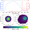 |
Fig. 1 Assumed instrumental response for the individual H.E.S.S. I telescopes. (a) indicates the total bandpass, where ɛ(λ) is defined as the ratio between detected and incident photons. For comparison, the night sky spectrum from Benn & Ellison (1998) is shown in red. (b) indicates the effective area for a pixel close to the optical axis. (c) indicates the effective area for an off-axis pixel. This suggests noticeable asymmetry due to optical aberrations. The white hexagons in (b) and (c) indicate the pixel size when projected onto the reference frame of the telescope. |
2.3 Telescope model
We focus our analysis on the H.E.S.S. CT1 telescope as an exemplar of the ‘third generation’ of IACTs. CT1 follows a Davies-Cotton design, with spherical mirrors arranged on a partial sphere with a radius corresponding to their focal length. In the case of CT1, there are 380 mirror facets with a diameter of 60 cm each, giving the telescopes an effective aperture of around 107 m2. The camera of the telescope consists of 960 PMTs acting as pixels, with Winston cones concentrating the light onto them. Table 1 shows the specifications of H.E.S.S. CT1-4. With these optical components in the light path, the bandpass of the telescope can be described by
 (26)
(26)
where R is the mirror reflectivity, E is the Winston cone efficiency, and P is the photon detection efficiency. While these might vary between individual mirrors, Winston cones, and PMTs, in the context of this work, we assumed a shared bandpass for all components. Figure 1 shows the bandpass for the H.E.S.S. I telescopes, calculated from R(2) and E(λ) given in Bernlöhr et al. (2003), and P(2) in Bernlöhr (2008). To accountfor differences between PMTs to first order, we performed a quasi-flatfielding procedure outlined in Sect. 3.2. Additionally, a factor of 0.8 is applied to account for telescope degradation compared to the nominal design value of the optical efficiency (Schäfer 2023).
The optical PSF is similar to the pixel size of 0.02 square degrees for CT1-4, but suffers from optical aberrations for off- axis light. To determine the response of pixels to light, we utilised ray-tracing to determine the amount of light hitting a pixel depending on the coordinate of the point source in the telescope frame, resulting in an effective area for each coordinate and pixel. Figure 1 shows the resulting effective area for a pixel close to the optical axis and at the edge of the telescope, highlighting the effect of the off-axis optical aberrations. New generation IACT designs, such as the Schwarzschild-Couder design for the CTAO SST telescopes, suffer less from these off- axis aberrations as a result of their two-mirror design (Giro et al. 2017).
The PSF model does not account for telescope deformation or changes to the PMT response over time (besides the Flatfielding coefficients). However, the optical PSF of the H.E.S.S. telescopes has proven to be remarkably stable (2024, priv. com- mun.), and deformations are small for altitude angles above 40° (Cornils et al. 2003). We implemented all discussed models in an open-source software package called nsb24. Depending on the observed star field, simulations run at a speed of around 1 Hz.
3 Application to H.E.S.S
As the readout windows of the H.E.S.S. telescopes are of the order of nanoseconds and the typical NSB rates are of the order 50 MHz to 1000 MHz, the integrated NSB signal in a single Cherenkov shower event image is too low for a statistical comparison to the simulation data. Therefore, for H.E.S.S. CT1-4, the following procedure was used to estimate the NSB in a pixel:
For each event image, determine all pixels containing Cherenkov light by checking if it or its neighbours are above a determined threshold.
For each event image, read out the intensity value for each pixel determined not to contain Cherenkov light. This is called the pedestal value.
When there is enough data for each pixel, the root-meansquare (RMS) of these pedestal values is determined.
As the CT1-4 PMTs are coupled via alternating current (AC) to their samplers, the mean pedestal value of a CT1 pixel is NSB-independent and cannot be used to determine incident NSB. Since higher NSB does result in larger fluctuations in the pedestal distribution, the RMS can be related to the NSB rate by (Aharonian et al. 2004)
 (27)
(27)
where RMSp is the pedestal RMS, RMS0 is the electronic pedestal in the absence of illumination,  is the charge dispersion of a single photoelectron, and τ is the readout window. To gain enough pedestal values per pixel to determine the RMS accurately takes around 8 s in CT1-4. For CT5, a more accurate method can be used due to its direct current (DC) coupling, which in principle enables the NSB readout up to event-wise rates, see Werner et al. (2017). For CT1-4, the expected relative error on the resulting NSB rate FOBS is within 10% to 20% (Aharonian et al. 2004). For each pixel, FOBS can then be directly compared with the simulated NSB rate FSIM for each readout window.
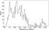 |
Fig. 2 Distribution of mean FOBS over all pixels for each run. Galactic fields are found towards the upper end, and extragalactic fields are at the lower end. |
3.1 The NSB dataset
As mentioned in Sect. 2.3, we focused our analysis on the CT1 telescope. We used NSB data taken during 1 year of CT1 observations for our comparison. The time period is from June 8, 2020, until June 3, 2021. This was chosen to coincide with a period of time where extensive Monte-Carlo validation was performed for the H.E.S.S. instrument (Leuschner et al. 2024).
In total, this period contains 2618 observation runs for the CT1 telescope. To remove unwanted effects such as cloud coverage or unstable atmospheric conditions, we imposed quality cuts on this dataset: removing all runs where the telescope event rate fluctuated or drifted5 (indicators for clouds and/or unstable atmospheric conditions). We also removed all runs with a duration lower than 28 min, since premature cancellations of runs can be potentially indicative of problems during the run. We furthermore imposed a cut on the average altitude of each observation run to be above 40 deg, to stay in a regime where the optical PSF of the telescope is stable (Cornils et al. 2003). After all the cuts, 1231 observation runs remained, 97 of which were conducted during partial moonlight; the gain settings for the camera were the same during both modes of operation (Tomankova et al. 2022). The runs include both extragalactic and galactic observation positions and are distributed over the entire area of the sky observable to H.E.S.S. In total, there are 59 different observational fields present in this dataset. The mean NSB rate FOBS for runs varies between 60 MHz and 260 MHz (see Fig. 2).
3.2 Pointing correction and quasi-flatfielding
To ensure the best possible match between the data and the simulations, the simulated field was corrected using the H.E.S.S. pointing correction for each time period, which were estimated to be accurate within 8″ (Hinton & H.E.S.S. Collaboration 2004). These corrections rely on pointing runs taken monthly, during which the telescope is centred on guide stars and the deviation is recorded depending on altitude and zenith. Additionally, a refraction model is used to simulate the refraction of starlight.
While the H.E.S.S. telescopes acquire flatfielding data using LED flashers, we find that these data are unable to correct NSB images. This is most likely due to the different way the NSB data is captured compared to the way flatfielding for air shower observations by H.E.S.S. is performed (uniform exposure compared to short flashes). As such, we implemented a quasi-flatfielding technique:
We fitted an empirical scaling factor to each model component for each run. This is done to capture the influence of atmospheric conditions and airglow variability. To minimise the contribution of single pixel outliers, a soft_l1 loss function is used for the fit. This is defined as
 (28)
(28)We then performed a linear fit for each individual pixel, again using a soft_l1 loss function to remove the influence of single pixel outliers. We applied this fit for three different time periods, necessitated by PMT gain changes during the year affecting pixel response (see Fig. 3).
For this quasi-flatfielding, we excluded runs with Eta Carinae in the FoV, since the bright nebulae component is not captured by our model (see Sect. 4.1.3) and worsens the fit considerably. The data is then corrected using the determined linear coefficients (m, b) depending on the time period. The fitting results from step 1 can also be used to determine the airglow (Sect. 4.1.1) and atmospheric conditions (Sect. 4.1.2).
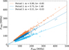 |
Fig. 3 Determination of flatfielding coefficients for a pixel close to the camera centre showing large changes between time periods. The coefficients are determined for three distinct time periods, to account for gain readjustment at the beginning of the periods. Each scatter point is an NSB data point determined during a run. The transition dates between periods are 2020-11-02 and 2021-04-29. This pixel is one of the most affected pixels. |
3.3 Comparison between simulation and NSB data
Figure 4 shows the comparison between telescope data (top row) and simulation (middle row) for four different astronomical fields6. Empty pixels (white) occurring in the top images are inactive pixels or were disabled during the observation because of the presence of a bright object. While the overall shape and inhomogeneity of the NSB data are well reproduced within the simulations, there are deviations from measurements of the order of up to 20 MHz for each run. These can most likely be explained by the inability of the diffuse contribution model to capture temporal variations, especially of the airglow component (see Sect. 4.1.1). The standard deviations of the residuals are of the order of 5% to 10%. These values are also representative of the total run selection, with the median standard deviation being 6.3%. Over the course of the year, the mean and standard deviation of the residuals are stable, see Fig. 5. Compared to the old approach, where the NSB rate was assumed to be uniform and stable at 134 MHz for non-moonlight runs, there is a clear improvement as seen in Fig. 6 (moonlight observation runs were excluded for this comparison). The central 90% range for our method is [−21%, +19%], while the 90% range for the old approach is [−64%, +48%].
4 Discussion
After introducing the NSB model and its components and describing its application to H.E.S.S. data, we now discuss the limitations of the model in the context of systematics and non-modelled effects (Sect. 4.1); commenting on the effects of airglow variability, atmospheric conditions, bright nebulae, and transient events. We also give a short overview of other possible contributions to NSB. In Sect. 4.2, we describe possible use cases of our new methodology.
4.1 Systematics and non-modelled effects
4.1.1 Airglow variability
As mentioned in Sect. 2.1.3, the airglow has been shown to vary on short (minutes) and long (monthly) timescales during a year (Khomich et al. 2008). Capturing these variations in a predictive model has proven difficult. To quantify the effect of these variations and the accuracy of our predictions, we used the fit to airglow normalisation from Sect. 3.2 to calculate the airglow strength for H.E.S.S. observations of an extragalactic field during the months of October and December 2020. We chose this field because the stellar and diffuse galactic contributions are low. It has also been observed multiple times per night and its distance from the celestial pole enables a zenith-dependent analysis.
As expected, we find strong variability in airglow intensity (see Fig. 7). There is a difference between the two months, with the average airglow in December at 46.5 MHz compared to 58.5 MHz in October. Additionally, there are night-to-night variations of the order of 10 MHz. On some nights, such as December 13, 2020, the airglow can vary of the order of 5 MHz within the time span of 1 hour. Given that the median NSB rate for each pixel is around 100 MHz, these variations could already be enough to explain the relative prediction error of the order of 12% (see Sect. 3.3). This also agrees with data taken by Preuss et al. (2002), who found the diffuse sky brightness to vary of the order of 10% on a nightly basis.
An unexpected discovery is the seeming independence of the airglow on the zenith angle at the H.E.S.S. site. As discussed in Sect. 2.1.3, a positive correlation of airglow intensity with zenith angle is expected due to the van Rhijn effect (van Rhijn 1921). Comparing the measured airglow values with the model taken from Noll et al. (2012), there seems to be very little correlation. Interestingly, this is also consistent with the observations by Preuss et al. (2002), who found the diffuse sky brightness of dark regions on the sky to be functionally independent of zenith angle at the H.E.S.S. site. This merits further study.
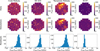 |
Fig. 4 Comparison between NSB measurements and simulation for the Crab nebula, SS 433, Tarantula nebula, and M 87. The upper row displays the data corrected for flatfielding, the middle row displays the simulated data, and the bottom row displays the pixel-wise residuals in MHz. White pixels in the top row indicate that this specific pixel was disabled at the time of data acquisition. |
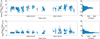 |
Fig. 5 Distribution of the mean and standard deviation of the relative residual |

4.1.2 Atmospheric conditions
Atmospheric conditions also have a large effect on the accuracy of the predictions. While the extinction/scattering effect due to Rayleigh scattering changes little, differences in aerosol concentration can lead to large variations in the contribution of stellar and lunar light to the NSB rate in IACTs, while having less of an effect on diffuse sources such as airglow and zodiacal light due to their lower effective scattering coefficient (see Sect. 2.2). Comparing the fitted stellar normalisation from Sect. 3.2 and daily (aerosol optical depth) AOD data from the AERONET site at the H.E.S.S. observatory, there is an observable correlation with Pearson correlation coefficient R = −0.63 (see Fig. 8). Since the AOD data is taken during the day, we applied a linear interpolation of the AOD values to estimate aerosol conditions during the night. While this provides a time-resolved approximation, reliance on daytime measurements may not fully capture potentially non-linear variations in AOD throughout the night. As such, deviations between predicted and actual conditions are expected, and a perfect correlation is not expected.
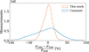 |
Fig. 6 Distribution of pixel-wise residuals over all pixels for the new method described in this work and the previous method of assuming a constant NSB over the entire FoV of 134 MHz for moonless nights. |
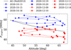 |
Fig. 7 Airglow fit from Sect. 4.1.2 for ten nights of observation of an extragalactic field. Here, the zenith range was larger than 15 deg. For comparison, the predicted value using the model from Noll et al. (2012) is plotted in black. |
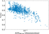 |
Fig. 8 Correlation between interpolated AOD at 380 nm, as determined during the day by the AERONET system at the H.E.S.S. site, and the normalisation of the stellar contribution, ɛstellar, as determined in (4.1.2). The Pearson correlation coefficient is R = −0.63. |
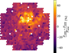 |
Fig. 9 Residual map of an observation of Eta Carinae. Due to the bright nebula component, the model fails to capture up to 50% of the NSB emission coming from the Carina nebula. For a H.E.S.S. gamma-ray source analysis corresponding to this observation, see H.E.S.S. Collaboration (2025). |
4.1.3 Bright nebulae
Due to its construction, the DGL model mainly captures the effect of strong forward scattering as expected in optically thick regions of interstellar dust (see Sect. 2.1.5). It is thus unable to capture the effect of bright diffuse emission by optically thick regions. As such, emission and reflection by nebulae is not captured by our model. For bright nebulae, this leads to a measurable underestimation of the flux. In the specific case of the Carina nebula, which is the brightest nebula visible in the night sky and a common target for the H.E.S.S. IACTs (see H.E.S.S. Collaboration 2012, 2020, 2025), this leads to the model being unable to capture up to 40% of the emission in the brightest regions of the nebula (see Fig. 9). Since the Carina nebula is more than an order of magnitude brighter than other nebulae, we expect the effect to be less pronounced for them.
4.1.4 Transient events and other time-dependent phenomena
While the model is able to capture most static components, transients such as satellites, meteors, novae, supernovae, and variable stars are not included. Currently, bright satellite or meteor trails affect a sub-percentage of observation time in H.E.S.S. (Lang et al. 2023), but with the emergence of large satellite constellations, this fraction is expected to rise continuously. They could possibly be modelled by using their two-line element sets and albedo, but since two-line element files describing satellite orbits become outdated quickly, these predictions would become inaccurate if done over time periods longer than a few days (Bassa et al. 2022). Meteor trails cannot be modelled due to their unpredictability. Another example of transient events are bright novae, such as RS Ophiuchi (H.E.S.S. Collaboration 2022). Such novae can be seen as bright residuals (see Fig. 10) of the order of hundreds of MHz. Variable stars are another issue, since their brightness can change compared to its value in stellar catalogues. For example, over the period of H.E.S.S. observations from 2004 to 2024, the star Eta Carinae has gone through significant changes in brightness (Martin et al. 2021). Modelling such stars correctly would require frequent catalogue updates or predictive modelling.
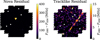 |
Fig. 10 Residuals caused by a nova and a track-like residual in the dataset, possibly due to a satellite (Lang et al. 2023). |
4.1.5 Other effects
There is a variety of other effects that could further affect the accuracy of this method. For example, it does not model planets or account for population centres. The closest population centre to the H.E.S.S. site in Namibia is Windhoek, which has a measurable effect in NSB measurements below an altitude of 55° (Preuss et al. 2002). For high-zenith observations, there is also the effect of direct illumination of the pixels due to ground reflections.
4.2 Use for IACT analyses
4.2.1 Instrument design
The ability to make per-pixel estimates of NSB in IACTs is useful for the design of future IACT projects, such as CTAO (Cherenkov Telescope Array Consortium et al. 2019). One possible area of application is the thermal design of IACT cameras, as high rates of NSB increase the thermal load of SiPMs better informing required cooling capacity and thermal safety margins (Spencer et al. 2024). In the context of instrument passbands, our model can be used to simulate the effect of wavelength filters and PMT choice on expected background rates for different astronomical fields. It is also applicable for the validation of future IACT calibration methods, such as in Abe et al. (2023), where the possibility of online pointing calibration using PMT currents was investigated.
4.2.2 Observation planning and instrument monitoring
Accurate simulations of the night sky are beneficial for the planning of IACT observations, especially under moonlight conditions. There are two main considerations: minimising the amount of pixels that need be turned off due to bright stars by choosing the correct field to image a source (since IACTs image most objects at an offset, the choice of field has a rotational freedom), and choosing fields during moonlit nights that reduce the total brightness in the detector (e.g. imaging low-brightness extragalactic targets during moonlit nights). Knowing the brightness in advance can inform the trigger threshold chosen for an observation, avoiding unstable trigger behaviour. It can also help to reduce the amount of turned-off pixels due to high NSB, by lowering the camera gain value based on the astronomical field (Bi et al. 2022). Accurate simulations also allow for the comparison of pixel currents or pixel pedestal values with simulated values to identify anomalies, while also enabling the monitoring of optical system degradation, atmospheric conditions (see Sect. 4.1.2), satellite trails (see Sect. 4.1.4), and PSF evolution directly from the telescope data over time.
4.2.3 Event classification and reconstruction
It is possible to augment conventional sim_telarray simulated images (without NSB) with predictions from our model. A variety of observational conditions could be simulated and used to create a more realistic training dataset for boosted decision tree analyses constructed for long-duration use in H.E.S.S.
A future work will discuss how to apply the newly modelled NSB maps to a full IACT analysis, from event images to source spectra. Our NSB tool is best suited for so-called run-wise analyses, whereby simulations are run to correspond to every 28 minutes of observing with H.E.S.S. (Holler et al. 2020). In this scenario, our tool would be used to generate a map of the average NSB experienced during this time period, and would then be summed with specialised simulations where no other NSB is simulated by packages such as sim_telarray (Bernlöhr 2008). Alternatively, one could think of a more conventionally binned analysis, whereby simulations are generated to represent an average 2D NSB structure in a particular zenith bin.
Deep learning classifiers are known to be particularly sensitive to NSB conditions (Shilon et al. 2019). A similar data augmentation approach as in the first paragraph could be used to reduce the discrepancy between the simulated training data and the IACT observations for supervised machine learning. Dellaiera et al. (2024) showed that tuning simulations with accurate NSB values for an observation leads to improved results, comparable or exceeding more complicated domain adaptation algorithms.
5 Conclusion
In this work, we presented a new method to estimate the NSB in IACTs on a per-pixel basis, inspired by techniques used to model the night sky in optical astronomy. We included the diffuse contributions of airglow, zodiacal light, scattered moonlight, and DGL, relying on models also used for optical astronomy and light pollution modelling (Noll et al. 2012; Jones et al. 2013; Masana et al. 2021; Winkler 2022). We also used GaiaDR3 (Gaia Collaboration 2023) and Hipparcos-Tycho ESA (1997) stellar data, relating it to synthetic stellar spectra from Coelho (2014) to calculate the expected contribution to per-pixel NSB employing ray-traced pixel effective areas. We accounted for atmospheric extinction and scattering using a single-scattering approximation, simplifying with an effective scattering coefficient when appropriate.
Comparing our simulation to the data from the CT1 telescope of H.E.S.S., we find good agreement between the two, with the central 90% range of the relative pixel-wise deviation for our method being [−21%, +19%], whereas assuming a constant rate results in a central 90% range of [−64%, +48%]. We find that there can be deviations of the order of 10% to 20%, which could potentially be explained by the variation in atmospheric conditions and the variability of the airglow.
We believe this to be the most sophisticated and accurate simulation of NSB for IACTs to date. A variety of ways it could prove useful to the IACT community are discussed in Sect. 4.2, including, but not limited to, observation planning and monitoring, instrument design, and studying the effect of NSB on event classification and reconstruction.
As discussed in Sect. 2.3, the tool and models used in this work will be released publicly. We believe this to be ofsignificant use to the community. We encourage other experiments such as MAGIC (Albert et al. 2008), VERITAS (Holder et al. 2008), MACE (Borwankar et al. 2024), F.A.C.T. (Biland et al. 2014), as well as the upcoming CTAO (Cherenkov Telescope Array Consortium et al. 2019), LACT (Zhang et al. 2025), and ASTRI Mini-Array (Vercellone et al. 2022) to follow our approach in future modelling of NSB. Our tool can easily be adapted to such instruments, given basic knowledge of, for example, the photon detection efficiency curve of the photomultipliers used in the camera.
Future studies could expand on the use cases mentioned in Sect. 4.2 and focus on using time-dependent airglow and atmospheric modelling to reduce the main uncertainties of our model further. They could also expand on the non-modelled effects discussed in Sect. 4.1, such as adding ground reflections, planets, and light pollution models.
Acknowledgements
This work has been through a review by the H.E.S.S. collaboration, who we thank for allowing us to use low level H.E.S.S. data in this work, and for useful discussions with collaboration members regarding this work (particularly Alison Mitchell, Simon Steinmaßl and the Innsbruck group). We also thank the other authors of Spencer et al. (2024) (particularly Rich White, who also provided feedback on this work) and Matthias Büchele for their previous research on this subject. We also thank Olivier Hainaut for useful discussions. STS is supported by the Deutsche Forschungsgemeinschaft (DFG, German Research Foundation) - Project Number 452934793. The telescope visualisations were done with ctapipe (Kosack et al. 2024; CTA et al. 2024). This work made use of Astropy7: a community-developed core Python package and an ecosystem of tools and resources for astronomy (Astropy Collaboration 2013, 2018, 2022). The authors furthermore thank the AERONET project and in particular, Kaleb Negussie as the principal investigator for their effort in establishing and maintaining the HESS AERONET site.
References
- Abe, K., Abe, S., Aguasca-Cabot, A., et al. 2023, A&A, 679, A90 [NASA ADS] [CrossRef] [EDP Sciences] [Google Scholar]
- Aharonian, F., Akhperjanian, A. G., Aye, K. M., et al. 2004, Astropart. Phys., 22, 109 [NASA ADS] [CrossRef] [Google Scholar]
- Aharonian, F., Ait Benkhali, F., Aschersleben, J., et al. 2024a, A&A, 686, A308 [NASA ADS] [CrossRef] [EDP Sciences] [Google Scholar]
- Aharonian, F., Benkhali, F. A., Aschersleben, J., et al. 2024b, ApJ, 970, L21 [Google Scholar]
- Ahnen, M. L., Ansoldi, S., Antonelli, L. A., et al. 2017, Astropart. Phys., 94, 29 [NASA ADS] [CrossRef] [Google Scholar]
- Albert, J., Aliu, E., Anderhub, H., et al. 2008, ApJ, 674, 1037 [CrossRef] [Google Scholar]
- Ashton, T., Backes, M., Balzer, A., et al. 2020, Astropart. Phys., 118, 102425 [NASA ADS] [CrossRef] [Google Scholar]
- Astropy Collaboration (Robitaille, T. P., et al.) 2013, A&A, 558, A33 [NASA ADS] [CrossRef] [EDP Sciences] [Google Scholar]
- Astropy Collaboration (Price-Whelan, A. M., et al.) 2018, AJ, 156, 123 [Google Scholar]
- Astropy Collaboration (Price-Whelan, A. M., et al.) 2022, ApJ, 935, 167 [NASA ADS] [CrossRef] [Google Scholar]
- Bassa, C. G., Hainaut, O. R., & Galadí-Enríquez, D. 2022, A&A, 657, A75 [NASA ADS] [CrossRef] [EDP Sciences] [Google Scholar]
- Benn, C. R., & Ellison, S. L. 1998, New A Rev., 42, 503 [Google Scholar]
- Bernlöhr, K. 2008, Astropart. Phys., 30, 149 [CrossRef] [Google Scholar]
- Bernlöhr, K., Carrol, O., Cornils, R., et al. 2003, Astropart. Phys., 20, 111 [Google Scholar]
- Bi, B., Barcelo, M., Bauer, C., et al. 2022, in PoS ICRC2022, 743 [Google Scholar]
- Biland, A., Bretz, T., BuB, J., et al. 2014, J. Instrum., 9, P10012 [Google Scholar]
- Bogumil, K., Orphal, J., Homann, T., et al. 2003, J. Photochem. Photobiol. A: Chem., 157, 167 [Google Scholar]
- Borwankar, C., Sharma, M., Hariharan, J., et al. 2024, Astropart. Phys., 159, 102960 [Google Scholar]
- Büchele, M. 2020, PhD thesis, FAU Erlangen, Germany [Google Scholar]
- Cherenkov Telescope Array Consortium, Acharya, B. S., Agudo, I., et al. 2019, Science with the Cherenkov Telescope Array (World Scientific) [Google Scholar]
- Coelho, P. R. T. 2014, MNRAS, 440, 1027 [Google Scholar]
- Cornils, R., Gillessen, S., Jung, I., et al. 2003, Astropart. Phys., 20, 129 [Google Scholar]
- CTA, Abe, K., Abe, S., et al. 2024, in PoS ICRC2024, 703 [Google Scholar]
- Dellaiera, M., Plard, C., Vuillaume, T., Benoit, A., & Caroff, S. 2024, arXiv e-prints [arXiv:2403.13633] [Google Scholar]
- Dumont, R., & Sanchez, F. 1976, A&A, 51, 393 [Google Scholar]
- ESA 1997, ESA Special Publication, 1200, The HIPPARCOS and TYCHO catalogues. Astrometric and photometric star catalogues derived from the ESA HIPPARCOS Space Astrometry Mission [Google Scholar]
- Fabricius, C., Luri, X., Arenou, F., et al. 2021, A&A, 649, A5 [NASA ADS] [CrossRef] [EDP Sciences] [Google Scholar]
- Gaia Collaboration (Prusti, T., et al.) 2016, A&A, 595, A1 [NASA ADS] [CrossRef] [EDP Sciences] [Google Scholar]
- Gaia Collaboration (Vallenari, A., et al.) 2023, A&A, 674, A1 [NASA ADS] [CrossRef] [EDP Sciences] [Google Scholar]
- Garstang, R. H. 1991, PASP, 103, 1109 [Google Scholar]
- Giavitto, G., Bonnefoy, S., Ashton, T., et al. 2017, in PoS ICRC2017, 301, 805 [Google Scholar]
- Giles, D. M., Sinyuk, A., Sorokin, M. G., et al. 2019, Atmos. Meas. Tech., 12, 169 [CrossRef] [Google Scholar]
- Giro, E., Canestrari, R., Sironi, G., et al. 2017, A&A, 608, A86 [NASA ADS] [CrossRef] [EDP Sciences] [Google Scholar]
- Górski, K. M., Hivon, E., Banday, A. J., et al. 2005, ApJ, 622, 759 [Google Scholar]
- Griffin, S., & VERITAS Collaboration. 2015, in PoS ICRC2015, 34, 989 [Google Scholar]
- Henyey, L. G., & Greenstein, J. L. 1941, ApJ, 93, 70 [Google Scholar]
- H.E.S.S. Collaboration (Abramowski, A., et al.) 2012, MNRAS, 424, 128 [NASA ADS] [CrossRef] [Google Scholar]
- H.E.S.S. Collaboration (Abdalla, H., et al.) 2020, A&A, 635, A167 [NASA ADS] [CrossRef] [EDP Sciences] [Google Scholar]
- H.E.S.S. Collaboration (Aharonian, F., et al.) 2022, Science, 376, 77 [NASA ADS] [CrossRef] [Google Scholar]
- H.E.S.S. Collaboration (Aharonian, F., et al.) 2024a, Science, 383, 402 [NASA ADS] [CrossRef] [Google Scholar]
- H.E.S.S. Collaboration (Aharonian, F., et al.) 2024b, A&A, 685, A96 [NASA ADS] [CrossRef] [EDP Sciences] [Google Scholar]
- H.E.S.S. Collaboration (Aharonian, F., et al.) 2025, A&A, 694, A328 [Google Scholar]
- Hinton, J. A., & H.E.S.S. Collaboration 2004, New A Rev., 48, 331 [Google Scholar]
- Holder, J., Acciari, V. A., Aliu, E., et al. 2008, in AIP Conf. Proc., 1085 (AIP), 657 [Google Scholar]
- Holler, M., Lenain, J. P., de Naurois, M., Rauth, R., & Sanchez, D. A. 2020, Astropart. Phys., 123, 102491 [NASA ADS] [CrossRef] [Google Scholar]
- Jones, A., Noll, S., Kausch, W., Szyszka, C., & Kimeswenger, S. 2013, A&A, 560, A91 [NASA ADS] [CrossRef] [EDP Sciences] [Google Scholar]
- Kawara, K., Matsuoka, Y., Sano, K., et al. 2017, PASJ, 69, 31 [NASA ADS] [CrossRef] [Google Scholar]
- Khomich, V. Y., Semenov, A. I., & Shefov, N. N. 2008, Airglow as an Indicator of Upper Atmospheric Structure and Dynamics (Springer) [Google Scholar]
- Kieffer, H. H., & Stone, T. C. 2005, AJ, 129, 2887 [NASA ADS] [CrossRef] [Google Scholar]
- Kocifaj, M. 2009, Solar Energy, 83, 1914 [Google Scholar]
- Kosack, K., Linhoff, M., Watson, J., et al. 2024, https://doi.org/10.5281/zenodo.14193232 [Google Scholar]
- Krisciunas, K., & Schaefer, B. E. 1991, PASP, 103, 1033 [Google Scholar]
- Kwon, S. M., Hong, S. S., & Weinberg, J. L. 2004, New A, 10, 91 [Google Scholar]
- Lang, T., Spencer, S. T., & Mitchell, A. M. W. 2023, A&A, 677, A141 [NASA ADS] [CrossRef] [EDP Sciences] [Google Scholar]
- Leckner, B. 1978, Solar Energy, 20, 143 [Google Scholar]
- Leinert, C., Bowyer, S., Haikala, L. K., et al. 1998, A&AS, 127, 1 [NASA ADS] [CrossRef] [EDP Sciences] [Google Scholar]
- Leuschner, F., Schäfer, J., Steinmassl, S., et al. 2024, in PoS Gamma2022, 231 [Google Scholar]
- Martin, J. C., Davidson, K., Humphreys, R. M., & Ishibashi, K. 2021, RNAAS, 5, 197 [Google Scholar]
- Masana, E., Carrasco, J. M., Bará, S., & Ribas, S. J. 2021, MNRAS, 501, 5443 [NASA ADS] [CrossRef] [Google Scholar]
- Noll, S., Kausch, W., Barden, M., et al. 2012, A&A, 543, A92 [NASA ADS] [CrossRef] [EDP Sciences] [Google Scholar]
- Patat, F. 2008, A&A, 481, 575 [NASA ADS] [CrossRef] [EDP Sciences] [Google Scholar]
- Preuss, S., Hermann, G., Hofmann, W., & Kohnle, A. 2002, Nucl. Instrum. Methods Phys. Res. A, 481, 229 [Google Scholar]
- Puehlhofer, G., Bernlöhr, K., Bi, B., et al. 2022, in PoS ICRC2022, 764 [Google Scholar]
- Rieke, G. H., Blaylock, M., Decin, L., et al. 2008, AJ, 135, 2245 [NASA ADS] [CrossRef] [Google Scholar]
- Schlegel, D. J., Finkbeiner, D. P., & Davis, M. 1998, ApJ, 500, 525 [Google Scholar]
- Schafer, J. 2023, PhD thesis, FAU Erlangen, Germany [Google Scholar]
- Shilon, I., Kraus, M., Büchele, M., et al. 2019, Astropart. Phys., 105, 44 [NASA ADS] [CrossRef] [Google Scholar]
- Spencer, S., Watson, J. J., Giavitto, G., Cotter, G., & White, R. 2024, in PoS Gamma2022, 218 [Google Scholar]
- Toller, G. N. 1981, PhD thesis, SUNY Stony Brook, New York, USA [Google Scholar]
- Tomankova, L., Yusafzai, A., Kostunin, D., et al. 2022, Gain settings for the upgraded H.E.S.S. CT1-4 cameras under moonlight observations, Tech. rep., High Energy Steroscopic System [Google Scholar]
- van Rhijn, P. J. 1921, Publ. Kapteyn Astron. Lab. Groningen, 31, 1 [Google Scholar]
- Vercellone, S., Bigongiari, C., Burtovoi, A., et al. 2022, JHEAP, 35, 1 [Google Scholar]
- Wenger, M., Ochsenbein, F., Egret, D., et al. 2000, A&AS, 143, 9 [NASA ADS] [CrossRef] [EDP Sciences] [Google Scholar]
- Werner, F., Bauer, C., Bernhard, S., et al. 2017, Nucl. Instrum. Methods Phys. Res. A, 876, 31 [CrossRef] [Google Scholar]
- Winkler, H. 2022, MNRAS, 514, 208 [Google Scholar]
- Zhang, Z., Yang, R., Zhang, S., et al. 2025, Chinese Phys. C, 49, 035001 [Google Scholar]
Data from https://www.spaceweather.gc.ca, accessed 2024-12-11.
For H.E.S.S. gamma-ray source analyses corresponding to these observations, see the following: the Crab nebula (Aharonian et al. 2024a), SS 433 (H.E.S.S. Collaboration 2024a), the Tarantula nebula (Aharonian et al. 2024b), and M87 (H.E.S.S. Collaboration 2024b).
All Tables
All Figures
|
Fig. 1 Assumed instrumental response for the individual H.E.S.S. I telescopes. (a) indicates the total bandpass, where ɛ(λ) is defined as the ratio between detected and incident photons. For comparison, the night sky spectrum from Benn & Ellison (1998) is shown in red. (b) indicates the effective area for a pixel close to the optical axis. (c) indicates the effective area for an off-axis pixel. This suggests noticeable asymmetry due to optical aberrations. The white hexagons in (b) and (c) indicate the pixel size when projected onto the reference frame of the telescope. |
| In the text | |
|
Fig. 2 Distribution of mean FOBS over all pixels for each run. Galactic fields are found towards the upper end, and extragalactic fields are at the lower end. |
| In the text | |
|
Fig. 3 Determination of flatfielding coefficients for a pixel close to the camera centre showing large changes between time periods. The coefficients are determined for three distinct time periods, to account for gain readjustment at the beginning of the periods. Each scatter point is an NSB data point determined during a run. The transition dates between periods are 2020-11-02 and 2021-04-29. This pixel is one of the most affected pixels. |
| In the text | |
|
Fig. 4 Comparison between NSB measurements and simulation for the Crab nebula, SS 433, Tarantula nebula, and M 87. The upper row displays the data corrected for flatfielding, the middle row displays the simulated data, and the bottom row displays the pixel-wise residuals in MHz. White pixels in the top row indicate that this specific pixel was disabled at the time of data acquisition. |
| In the text | |
|
Fig. 5 Distribution of the mean and standard deviation of the relative residual |
| In the text | |
|
Fig. 6 Distribution of pixel-wise residuals over all pixels for the new method described in this work and the previous method of assuming a constant NSB over the entire FoV of 134 MHz for moonless nights. |
| In the text | |
|
Fig. 7 Airglow fit from Sect. 4.1.2 for ten nights of observation of an extragalactic field. Here, the zenith range was larger than 15 deg. For comparison, the predicted value using the model from Noll et al. (2012) is plotted in black. |
| In the text | |
|
Fig. 8 Correlation between interpolated AOD at 380 nm, as determined during the day by the AERONET system at the H.E.S.S. site, and the normalisation of the stellar contribution, ɛstellar, as determined in (4.1.2). The Pearson correlation coefficient is R = −0.63. |
| In the text | |
|
Fig. 9 Residual map of an observation of Eta Carinae. Due to the bright nebula component, the model fails to capture up to 50% of the NSB emission coming from the Carina nebula. For a H.E.S.S. gamma-ray source analysis corresponding to this observation, see H.E.S.S. Collaboration (2025). |
| In the text | |
|
Fig. 10 Residuals caused by a nova and a track-like residual in the dataset, possibly due to a satellite (Lang et al. 2023). |
| In the text | |
Current usage metrics show cumulative count of Article Views (full-text article views including HTML views, PDF and ePub downloads, according to the available data) and Abstracts Views on Vision4Press platform.
Data correspond to usage on the plateform after 2015. The current usage metrics is available 48-96 hours after online publication and is updated daily on week days.
Initial download of the metrics may take a while.