| Issue |
A&A
Volume 699, July 2025
|
|
|---|---|---|
| Article Number | A161 | |
| Number of page(s) | 8 | |
| Section | Stellar atmospheres | |
| DOI | https://doi.org/10.1051/0004-6361/202553688 | |
| Published online | 07 July 2025 | |
Making sense of the spectral line profiles of Betelgeuse and other red supergiants★
1
IRAP, Université de Toulouse, CNRS, CNES,
UPS. 14, Av. E. Belin,
31400
Toulouse,
France
2
IRAP, Université de Toulouse, CNRS, CNES,
UPS. 57, Av. d’Azereix,
65000
Tarbes,
France
★★ Corresponding author.
Received:
7
January
2025
Accepted:
24
April
2025
Abstract
Spectropolarimetry of atomic lines in the spectra of Betelgeuse and other red supergiants (RSG) typically presents broad line profiles in linear polarization, but narrow profiles in intensity. By contrast, recent observations of the RSG RW Cep show broad intensity profiles, comparable to those in linear polarization. This observation suggests that the difference in the Stokes Q/U and I profile widths noted in many RSGs arises from the temporary atmospheric conditions of a given star. We propose an explanation for both cases based on the presence of strong velocity gradients steeper than the thermal broadening of the spectral line. Using simple analytical radiative transfer, we computed intensity line profiles in such scenarios. We find that they qualitatively match the observed broadenings: steep gradients are required for the narrow profiles of Betelgeuse, while shallow gradients are required for the broad profiles of RW Cep. Profile bisectors are also reasonably well explained by this scenario, despite the simple radiative transfer treatment used. These results give a comprehensive explanation of the intensity and polarization profiles. They also support the approximation of a single-scattering event used to explain the observed linear polarization in images inferred for the photosphere of Betelgeuse and other RSGs such as RW Cep, µ Cep and CE Tau. The atmospheres of RSGs appear capable, perhaps cyclically, of either producing steep velocity gradients that prevent photospheric plasma from reaching the upper atmosphere and thus hinder major mass-loss events, or allowing vertical movements to proceed unchanged, enabling plasma to rise, escape gravity, and form large dust clouds in the circumstellar environment. The origin of the velocity gradient and its modulation within the atmosphere remains an open question.
Key words: radiative transfer / stars: atmospheres / supergiants
Based on observations obtained at the Télescope Bernard Lyot (TBL) at Observatoire du Pic du Midi, CNRS/INSU and Université de Toulouse, France.
© The Authors 2025
 Open Access article, published by EDP Sciences, under the terms of the Creative Commons Attribution License (https://creativecommons.org/licenses/by/4.0), which permits unrestricted use, distribution, and reproduction in any medium, provided the original work is properly cited.
This article is published in open access under the Subscribe to Open model. This email address is being protected from spambots. You need JavaScript enabled to view it. to support open access publication.
1 Introduction
The discovery of linear polarization in the atomic lines in the spectrum of Betelgeuse (Aurière et al. 2016) enabled a successful imaging technique that has continuously provided images of the convective structures in the photosphere of Betelgeuse (López Ariste et al. 2018) and other red supergiants (RSG) such as µ Cep (López Ariste et al. 2023) or CE Tau since 2013 (López Ariste et al. 2018). More recently, 3D images of the photosphere, exploiting the different formation heights of atomic lines, have been inferred from these spectropolarimetric signals (López Ariste et al. 2022). Beyond these images, this technique has identified the high convective velocities predicted by numerical simulation codes and confirmed the size and temporal scales of variation of these convective structures. The measurement of plasma velocities at different heights has also identified plasma plumes with nearly constant velocity as they rise through Betelgeuse’s atmosphere. This points to the presence of an acceleration mechanism – hitherto unidentified – from photospheric heights that balances gravity and maintains plasma velocities as the plasma plumes reach the height at which they escape as stellar wind.
These successes are based on a series of approximations regarding polarized line formation, discussed and partially justified in the literature cited above. Among these, perhaps the weakest approximation is the imposition of a relationship between brightness and vertical velocity. Such a correlation is observed when line formation takes place in areas where convection remains the dominant dynamical process, as is the case with the Sun. Numerical simulations of Betelgeuse’s photosphere (Kravchenko et al. 2019) affirm such a relationship. Moreover, they suggest that the region of atomic line formation in the spectrum resides well above the convective zone and, thereby, do not support a clear correlation between brightness and velocity in the formation of spectral lines in Betelgeuse. This prediction is challenged by the comparison between images inferred from spectropolarimetry – assuming the correlation holds true – and the reconstructed images obtained through interferometry.
Kravchenko et al. (2018) explored whether convection leaves a signature in the intensity spectra and, through a newly-developed tomographic technique, identified a hysteresis loop reminiscent of what would be expected if lines were formed under convective conditions – that is, when the correlation between brightness and vertical velocities remains valid. Such hysteresis loops may be seen in observed spectra and also, marginally, in synthetic spectra computed by radiative transfer through numerically simulated stellar snapshots. However, as the authors claim, hysteresis loops may not necessarily indicate line formation where convection takes place and rather imply that acoustic waves or pulsations can propagate such correlations to selected patches well above where convection imposes those relationships between brightness and vertical velocity. Since, convection has typically been cited as an explanation for C-shape line asymmetries (Gray 2008), it follows that the intensity profile is appropriate for examining the validity of the brightness-velocity correlation, which is central to interpreting the measured linear polarization in terms of images of convective structures.
However, inspection of the observed intensity and linear polarization profiles reveals that the challenges with intensity profiles extend beyond correctly interpreting bisectors or hysteresis loops. As emphasized by López Ariste et al. (2022), the intensity profiles observed on Betelgeuse are astonishingly narrower than the width of the linear polarization signal. This is illustrated in Fig. 1, where the limits of v∗, the assumed velocity of the star, and vmax, the assumed highest velocity of the rising plasma are shown. These two limits are established through simple inspection of the accumulated data set of linear polarization profiles. In a model of pure convective movements, all plasma that is bright rises vertically, and thereby the most blueshifted signal observed must originate from plasma rising close to the disk center at the maximum possible velocity. Thus, linear polarization cannot be observed at shorter wavelengths than this vmax limit. Similarly, plasma located at the limb of the star emits at zero velocity with respect to the bulk star velocity v∗. This red limit is not absolute: sinking plasma, although darker than rising plasma, can produce signals that are redder than this limit. However, these zones lead to very low emission. López Ariste et al. (2023) found that the spectra of the RSG µ Cep presented strong polarization signals beyond the red wing of the line profile and interpreted them as due to the intermittent plumes arising in the back hemisphere of the star, but rising high enough to be visible above the limb. But beyond these episodic phenomena, no large signals are observed to the red. López Ariste et al. (2022) discussed at length the validity and justification of these two velocities for Betelgeuse. Regardless of the actual value of these two velocities, what concerns us here is the considerable amount of linear polarization occurring at wavelengths that – judging from the intensity profile alone – lie in the continuum, beyond the blue wing of the line. It is difficult to interpret this observation. Continuum is precisely defined by its near-independence from wavelength, at least on the scales considered here. The observed linear polarization signal varies rapidly with wavelength and cannot be attributed to any continuum-emitting process. Interpreting it as polarization arising from the extreme wing of the spectral line is also implausible. Such an explanation would require 10% polarization levels at certain wavelengths, which is unrealistic. There is no known mechanism that could generate such high levels of linear polarization in the extreme wing of the line, when the observed polarization amplitudes in the line are 0.1% at most.
We address this issue in the present study. We propose a mechanism by which the intensity profile narrows after integrating over the disk, while the linear polarization profile retains its original width. Such a mechanism relies on two ingredients. The first is that, in the absence of stellar rotation and in an atmosphere with predominantly vertical plasma velocities, disk integration favors signals emerging from the disk center. This is because the emission wavelength is modulated by its projection onto the line of sight, and the cos θ function reaches a maximum at disk center. Hence, velocities around disk center, if relatively homogeneous, are similar and add up together, while, at the limb, a small change in position considerably alters the projected velocity, even if the atmosphere is homogeneous. This effect is common to all disk integrations; therefore, by itself, it does not distinguish Betelgeuse from any other star. The second ingredient is critical: it requires velocity gradients in the line formation region that exceed the width of the local line. Such gradients are expected in a convecting atmosphere characterized by large vertical velocities and shock waves. They deform the line profiles giving them a triangular shape (Bertout & Magnan 1987). As a result, and in sum, regions at disk center with large gradients produce triangular shape profiles that contribute across all wavelengths, while regions at the limb with low gradients produce narrow Gaussian profiles centered at near zero velocities, around υ∗. The correct combination of these contributions produces the observed profiles, as demonstrated in the following section.
In the process to understand the intensity profiles of Betelgeuse, a key element is the observation of another star, RW Cep. This star is not particularly different from Betelgeuse; although it is perhaps better classified as a yellow hypergiant (Anugu et al. 2024), the characteristics and evolution of the photosphere are identical. Any observational differences between Betelgeuse, RW Cep, or any similarly evolved giant star must be attributed primarily to the star’s current state: whether it is quietly convecting, as Betelgeuse appears to be (except perhaps during the recent Great Dimming event), or, on the contrary, whether it is in a Decin stage as RW Cep or µ Cep, experiencing repeated episodes of large plumes rising high enough to escape gravity and form new shells of dust clumps (López Ariste et al. 2023; Decin et al. 2006). It was therefore a major surprise to discover that, in our 2023 observations, RW Cep exhibits a large and broad intensity profile – fully compatible with the linear polarization signals and unlike anything observed in Betelgeuse over the past 10 years. RW Cep currently displays activity, which broadens its profiles. We were led to conclude that atmospheric dynamics, in the broadest sense, can either broaden or narrow intensity profiles. The narrow profiles observed in Betelgeuse are not intrinsic to an RSG. Rather, they are due to the present dynamics of the star. This insight led to the solution we propose. In Section 3, we explore how our hypothesis based on velocity gradients accounts for the intensity profiles of Betelgeuse and RW Cep.
In Section 4, we discuss and model one final observational fact. Bisectors of Betelgeuse line profiles often present a typical C-shape. Nevertheless, from time to time, they reverse their asymmetry. Our proposed solution aims to explain this difference and their change in time.
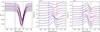 |
Fig. 1 Profiles of Betelgeuse observed from November 27, 2013, to March 3, 2015, with Narval at the TBL. The red vertical dashed line marks the chosen reference velocity υ∗ interpreted as the velocity of the star’s center of mass. The blue dashed line marks the maximum vertical velocity υmax of the plasma. |
2 Radiative transfer in the photosphere of an RSG
Our approach to the problem of radiative transfer in these atmospheres is guided by a constraint and a motivation. The constraint is that, despite the successes of numerical simulations and their promise of ever greater and precise detail, we cannot yet consider them the ultimate description of red supergiants. This is not only because we lack sufficient simulations with the appropriate parameters, but also because we must consistently check these models rather than assume their correctness and limit observations to a perennial validation. Our motivation is to seek an explanation rather than a description or a perfect fit. Our goal is not to quantitatively reproduce the intensity profiles, but to identify the key physical ingredients responsible for the main observed features.
With these criteria in mind, we boldly split the problem of radiative transfer into two classes. The first concerns the variation of opacity with time and position, both along and across the photosphere of our RSG. The second involves the integration of local line profiles along each line of sight and the addition of all the lines of sight over the stellar disk – what we refer to as the geometric aspect of the radiative transfer problem. If we conduct full radiative transfer on a numerical simulation, both aspects of the problem – geometry and opacity – are inevitably coupled, and we lose perspective on their relative importance. As observed, geometry is sufficient to explain the main features observed in the atomic line profiles of Betelgeuse. Since the geometric aspect is ever present and provides sufficient explanation, opacity variations play a secondary role – if not in their quantitative aspects, then at least in their mere presence.
We therefore reduce the transfer problem to its bare bones. We assume that opacity is constant along the line of sight and over the stellar disk, despite the clear variations in density and temperature. We assume a normalized continuum emitted below the line formation region. We parameterize this region with a geometrical distance z, which varies from 0 through 1, with z = 0 marking the strict bottom end of the region of formation and z = 1 marking the strict top end. At each line of sight, the emergent spectrum is given by
![Mathematical equation: \[I(v) = {e^{ - \tau (v)}},\]](/articles/aa/full_html/2025/07/aa53688-25/aa53688-25-eq1.png) (1)
(1)
where τ (ν) is the total opacity along the line of sight. We parameterize wavelength in terms of velocity differences υ with respect to the local reference frame of the star’s center of mass υ∗, such that υ = 0 km s−1. The total opacity is computed according to
![Mathematical equation: \[\tau (v,\theta ,\chi) = {\smallint ^}_{z = 0}^{z = 1}k\phi [v - v(z,\theta ,\chi )\cos \theta ]dz,\]](/articles/aa/full_html/2025/07/aa53688-25/aa53688-25-eq2.png) (2)
(2)
where k is the constant absorption coefficient, and υ(z, θ, χ) is the radial velocity of the atoms at height z, angular distance to the disk center θ, and position angle χ. Lastly, we approximate the line profile ϕ with a simple Gaussian of standard deviation Δ = 6 km s−1 (López Ariste et al. 2018), as defined by
![Mathematical equation: \[\phi (v) = {e^{ - \frac{{{v^2}}}{{{{\rm{\Delta }}^2}}}}}.\]](/articles/aa/full_html/2025/07/aa53688-25/aa53688-25-eq3.png) (3)
(3)
The local intensity profiles, integrated over z, for each position over the disk (θ, χ), are added together to produce the disk-integrated line profile, which we compare to the observations.
Our approach is guided by the work of Bertout & Magnan (1987) (see also Wagenblast et al. 1983 and Chandrasekhar 1945) in interpreting the doubling profiles periodically observed in Mira stars. The authors cited here stripped radiative transfer to its bare fundamentals to demonstrate the unexpected result of combining disk integration and velocity gradients along the line of sight. In their work, they addressed Mira stars, whose atmosphere is consists of an expanding (or contracting) shell of gas on top of the star. This shell is assumed to be homogeneous in velocity and geometry, which allows the integral over the disk to be closely intertwined with the integral along the line of sight. This assumption underpins their solution to the problem. In our present case, we also invoke strong velocity gradients along the line of sight, but these occur only in coincidence with the plumes of hot, rising plasma, and are neither homogeneous in their distribution over the disk nor in their velocities. For this reason, we decouple the integration along the line of sight from the integration over the disk. In this aspect, we diverge from the work of Bertout & Magnan (1987). Despite this difference, we recover most of the features described by these authors.
It is worthwhile to solve analytically the integral in Eq. (2) for several velocity gradients with respect to z. In the first and most straightforward case, the velocity υ0 is constant with z for all points on the disk, but projects onto the line of sight. We find that
![Mathematical equation: \[\tau (v,\theta) = k\left( {{z_1} - {z_0}} \right)\phi \left[ {v - {v_0}\cos \theta } \right].\]](/articles/aa/full_html/2025/07/aa53688-25/aa53688-25-eq4.png) (4)
(4)
As one adds profiles for different values of θ, one obtains a flat-bottom, or square, integrated profile. With limb darkening, this flat-bottom profile becomes highly asymmetric as can be seen in the left of Fig. 2. This result is expected for a constant and homogeneous rising velocity of the plasma. However, this is not observed, nor does one expect the velocity to be constant with z.
Hence, our second case assumes a linear dependence of velocity on z, given by υ(z) = υ0(1 − z), which ensures that the velocity diminishes with height. The integral is given by
![Mathematical equation: \[\tau (v,\theta) = \frac{{{\rm{\Delta }}k}}{{{v_0}\cos \theta }}\frac{{\sqrt \pi }}{2}\left[ {{\rm{erf}}\left( {\frac{v}{{\rm{\Delta }}}} \right) - {\rm{erf}}\left( {\frac{{v - {v_0}\cos \theta }}{{\rm{\Delta }}}} \right)} \right],\]](/articles/aa/full_html/2025/07/aa53688-25/aa53688-25-eq5.png) (5)
(5)
where erf stands for the error function. Again, we assume this law applies uniformly over the disk, and the only angular dependence arises from the projection onto the line of sight. Whenever υ0 is smaller than Δ, the result is a slightly deformed Gaussian that adds up for all points on the disk. However, if υ0 is larger than Δ, we find that for large values of θ, near the limb, quasi-Gaussian profiles are produced, while near disk center, when cos θ ≈ 1, flat-bottomed profiles appear. Integrating over all values of θ results in a disk-integrated asymmetric profile as shown in the center plot of Fig. 2.
However, a linear dependence of the velocity on z is not what one would naively expect for plasma that is ballistically sent upward during convection. One rather typically expects a square root dependence, (e.g., ![Mathematical equation: \[v(z) = {v_0}\sqrt {1 - \beta z} )\]](/articles/aa/full_html/2025/07/aa53688-25/aa53688-25-eq6.png) , where β modulates the final velocity of plasma. Such velocity may also be readily integrated, in which case the total opacity per line of sight is
, where β modulates the final velocity of plasma. Such velocity may also be readily integrated, in which case the total opacity per line of sight is
![Mathematical equation: \[\begin{array}{*{20}{l}} {\tau (v,\theta) = v\frac{{{\rm{\Delta }}k\sqrt \pi }}{{\beta v_0^2{{\cos }^2}\theta }}[erf\left( {\frac{{v - {v_0}\cos \theta \sqrt {1 - \beta } }}{{\rm{\Delta }}}} \right)}\\ {\,\,\,\,\,\,\,\,\,\,\, - {\rm{erf}}\left( {\frac{{v - {v_0}\cos \theta }}{{\rm{\Delta }}}} \right)]}\\ {\,\,\,\,\,\,\,\,\,\,\, + \frac{{k{{\rm{\Delta }}^2}}}{{\beta v_0^2{{\cos }^2}\theta }}\left( {{e^{ - \frac{{{{\left( {v - {v_0}\cos \theta \sqrt {1 - \beta } } \right)}^2}}}{{{{\rm{\Delta }}^2}}}}} - {e^{ - \frac{{{{\left( {v - {v_0}\cos \theta } \right)}^2}}}{{{{\rm{\Delta }}^2}}}}}} \right).} \end{array}\]](/articles/aa/full_html/2025/07/aa53688-25/aa53688-25-eq7.png) (6)
(6)
One readily notices the linear dependence on ν in the first term of this solution, a fact already pointed out by Bertout & Magnan (1987) in their geometric treatment and which persists despite the divergences between our two approaches. The resulting profiles, if this term dominates over the second, show a characteristic saw-toothed or triangular shape that is also seen in Fig. 2. The net result of summing these profiles with the usual Gaussian profiles arising close to the limb is a broadened but quasi-symmetric profile.
When changing the gradients of the velocity along the line of sight, even without modifying the maximum velocities involved (which are always 40 km s−1in the examples of Fig. 2) – we observe clear changes in the shape of the profiles. The examples in Fig. 2 illustrate how the disk-integrated line profile narrows or broadens. Furthermore, and in advance of the results in Sect. 4, we also see that the bisector is modified in these tests, without requiring changes in either the velocities or the absorption coefficient. The three examples in Fig. 2 show a typical C-shape bisector (no gradients case), an inverse C-shape bisector (linear gradients), and a quasi-vertical bisector (parabolic gradients). In summary, the combination of strong gradients with different dependence on z, brightness inhomogeneities, and disk integration appears to be necessary to reproduce the observed intensity profiles in different RSG.
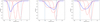 |
Fig. 2 Examples of profiles generated in the presence of strong gradients along the line of sight, and the resulting disk-integrated profiles. Left: profiles made in the absence of velocity gradients. The projection onto the line of sight shifts the position of the local profile. A simple limb-darkening law proportional to cos µ makes the summed profile asymmetric. Center: Employed linear velocity gradient. Right: gradient along the line of sight following a square-root law. In all cases, the same limb-darkening law as in the left panel is applied. Dashed red lines represent individual lines of sight from the disk center, θ = 45°, and close to the limb. Solid blue lines show the disk-integrated profile. Vertical dashed lines mark the radial outward velocity of the plasma, υ0 = υmax = −40 km s−1, in the observer’s frame, and the zero velocity υ∗. |
3 Reproducing the observed intensity profiles
Figures 1 and 3 show selected example profiles of Betelgeuse and RW Cep respectively, representing the two extremes of profile shapes observed in RSGs with Narval and its updated version, NeoNarval (see López Ariste et al. 2022; Donati et al. 2006, for a description of both instruments and data reduction procedures). Here, we present cross-correlation profiles made with the addition of many different spectral lines (Josselin & Plez 2007; Donati et al. 1997). Typically, these lines are combined irrespective of their line depression, formation height, or any other attribute. This is the approach used for the profiles shown in Fig. 3. In the case of Betelgeuse, the presented profiles date from 2013 and 2014. These data were previously presented by Aurière et al. (2016), who also discuss the line lists used in the cross-correlation. Since the Great Dimming event at the end of 2019, the levels of linear polarization in Betelgeuse have drastically diminished, even though it is observed periodically. As our purpose is to illustrate the difference in wavelength span between the linear polarization and the intensity profile, we adopted the older data to better illustrate this discrepancy. However, for the Neo-Narval data in 2023, the broadening difference between Stokes Q, U, and I remains unchanged. For our second star, RW Cep, we present NeoNarval data from August 18 to November 18, 2023.
As discussed, the presence of velocity gradients larger than the line width, and with different dependencies on z, gives rise to a variety of profile shapes – from purely Gaussian to saw-toothed, and from broad to narrow. The specific profile observed in an RSG at a given time depends on the distribution of both velocity gradients and brightness across the disk at the moment of the observation. For the sake of simplicity, we fix the gradients to be of the ballistic kind, with a square root dependence on z. However, we vary both the amplitude of the gradients (by changing the parameter β) and the distribution of brightness and velocity amplitudes across the disk. The parameter β is set constant for all points in disk. For the brightness and velocity distributions, we select the images inferred from the linear polarization of Betelgeuse to represent what we believe are acceptable distributions across the disk, recalling that both magnitudes – brightness and velocity – are determined in the inversion algorithms that fit the linear polarization as if the light-emitting plasma were subject to convection (López Ariste et al. 2018).
As a first illustration, using the image of the photosphere of Betelgeuse that best fits the observed linear polarization signals observed on November, 27, 2013, (Aurière et al. 2016) we present in Fig. 4 the local profiles along a radius across the stellar disk, together with the integrated profile observed by summing all those individual profiles. On that date, and along the chosen radius, not much contribution occurs at the maximum velocities. However, the plasma sinks at several points and appear redshifted with respect to the υ∗ velocity. In the figure, every local profile is normalized, and these redshifted points are easily spotted. They, nonetheless, barely contribute to the integrated profile, for its true intensity is low.
As described above, the profiles closest to the disk center contribute to the highest blueshifted velocities. Due to their velocity gradients, however, they also contribute at lower velocities. Profiles close to the limb contribute only to the lower velocity near the υ∗ rest velocity of the star. Altogether wave-lengths near this rest velocity receive a larger contribution in the integration, resulting in a narrow, blueshifted profile with the rest velocity υ∗ found in its red wing.
Based on this, we extend the calculation to the whole disk and explore the impact of the velocity gradients. Figure 5 shows the case of β = 1, where the velocity at each point decreases from the value found in the inferred image to zero across the span of the line formation region. This is quite a steep gradient near the disk center, with maximum velocities reaching 40 km s−1. However, the gradients reduce to zero toward the limb, and as a result the disk-integrated profile displays a combination of saw-toothed and Gaussian profiles as in Fig. 2. The brightness distribution, however, is not homogeneous, and some profiles are given more weight than others. This result is available in Fig. 5, where the ten observations, from November 27, 2013, to March 3, 2015, presented by Aurière et al. (2016) are used as examples of brightness and velocity spatial distributions. Notably, on this figure, the observed and computed profiles exhibit similar widths (of the order of 30 km/s).
We chose the opacity value k in Eq. (2) so that the disk-integrated profile matches the depth of the observed intensity profile. Otherwise, all the parameters adopted are those used by the inversion code to fit the linear polarization profiles: namely, the maximum velocity amplitude and the width of the Gaussian profile. A comparison of these computed and observed profiles is remarkable in terms of width and global shape. The computed profiles are narrow, despite the span of velocities used for the computation. This is due, as noted, to the combination of steep velocity gradients and the brightness distribution across the disk. Zero velocity falls on the line’s red wing rather than on its center. This justifies a posteriori the ad hoc choice made in the inversion codes by López Ariste et al. (2018). Here, this is an emergent feature; nothing in the computation forces the position of the minimum of the disk-integrated profile. The same can be said about the maximum velocity that falls over the continuum well beyond the blue wing of the line, despite the presence of high velocities at some points over the disk. We conclude from this comparison that our basic model captures the main features of the observed profiles of Betelgeuse. This is in spite of imposing a constant absorption coefficient through the atmosphere and the same velocity gradient dependence at all points. We later examine the bisector shape and velocity spans to further this comparison. At this point, however, we may venture to draw a far-reaching conclusion. The linear polarization model is based on the assumption that linear polarization emerges from Rayleigh scattering of the continuum. The continuum-polarized photons are subsequently absorbed by atoms higher in the atmosphere, which then re-emit them unpolarized. The local continuum polarization is in this manner erased in the spectral line, and it is this depolarization signal that we measure with our instruments. In this model, the polarization amplitude is primarily associated with the brightness of the continuum-emitting plasma, while the Doppler shift of the depolarized photon reflects that of the absorbing and re-emitting atom. Linear polarization profiles present a broad span of velocities, but the present comparison of computed and observed intensity profiles appears to require a gradient of velocities down to zero over the line formation region. We conclude therefore that the depolarized photons originate from the bottom of the formation region, while the photons forming the spectral line arise from integration over the entire region.
RW Cep represents the opposite extreme of the variation observed in the intensity profiles of RSGs. We see, in recent observations of this star, broadened profiles with a span comparable to the one observed in linear polarization profiles (Fig. 2). Josselin & Plez (2007) presented intensity profiles for RW Cep – though without linear polarization – that can be compared to those presented here to appreciate the variability which this RSG exhibits, in contrast to the stable profiles of Betelgeuse. In Fig. 6, we repeat the calculations of disk-integrated profiles using the same brightness and velocity distributions as for Betelgeuse in Fig. 5 (and therefore inferred from fitting the observed linear polarization of Betelgeuse), but with the value of β changed from 1 into 0.4. This value of β means that, rather than dropping to zero across the formation region of the spectral line, the velocity decreases by only 25%. With such shallow gradients, we recover broadened profiles that can be favorably compared to the observed profiles of RW Cep. Whenever the brightness distribution includes large hot spots across the disk, split profiles may appear, though these are not seen in the present observations of RW Cep.
This second favorable comparison between the broadened profiles resulting from weak gradients in our simple model and the observations of RW Cep provides further support. In our view, it confirms the hypothesis that the geometry of radiative transfer and, in particular, the combination of the brightness distribution and the actual gradients of velocity at the time of observation, are sufficient to qualitatively reproduce the observed intensity profiles. The presence of these deduced gradients is not unexpected. A convective atmosphere with acoustic waves traveling along and across it must exhibit strong velocity gradients.
The scenario for the polarized line formation that emerges from these tests is as follows: a continuum forms deep in the atmosphere of Betelgeuse (or any other RSG). This continuum is polarized by Rayleigh scattering, and at this stage, information about brightness inhomogeneities is transferred into the polarization amplitude. This does not have to be the continuum that ultimately emerges from the star, as the optical depth at continuum wavelengths may not yet be zero. It is depolarized by the line-forming atoms at the deepest point of its formation region. This is necessary as – according to our observations – linear polarization signals do not suffer from integration along the line of sight. Moreover, they retain the signature of the highest velocities found at the bottom of the line formation region. This supports the hypothesis that a single scattering event is responsible for creating the polarization signal. At this point in the optical path – where the line begins to form and depolarize a continuum that is itself still forming – the wavelength position of the polarization signal is set, which in turn determines its position over the stellar disk to which this polarization is assigned. Both the brightness of the image inferred from linear polarization and its position over the disk originate in this scenario from deep photospheric layers: the brightness from a deep continuum (well below the typical values of opacity of the emergent continuum), and the position over the disk from the first scattering event on a line-forming atom at the bottom of the formation region. From this point onward, the linear polarization profile remains unchanged, but the intensity profile continues to evolve as it moves along the line formation region, ultimately acquiring its final triangular or Gaussian shape at the top of the formation layer, where atmospheric velocities are significantly reduced.
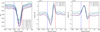 |
Fig. 3 Examples of RW Cep profiles observed with NeoNarval in 2023, with dates indicated in the legend. Intensity is shown in the left plot, while Stokes Q and U are displayed in the center and right plots, respectively. The red and blue vertical dashed lines mark the chosen values of υ∗ and υmax, respectively. |
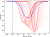 |
Fig. 4 Example of local (red) and integrated (blue) profiles along the vertical radius of the image of Betelgeuse that best fit the observations of linear polarization on December 20, 2013. All profiles are normalized to the continuum value for clarity in the plot. |
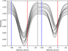 |
Fig. 5 Left: inferred images of Betelgeuse from November 27, 2013, to March 3, 2015, used to integrate profiles under the assumption that, at every point, the gradient is such that the velocity reduces to 0 at the top of the line formation region (β = 1). Profiles are shifted in ordinates for clarity. Right: observed intensity profiles from those same dates. |
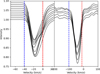 |
Fig. 6 Left: same as Fig. 5, but for β = 0.4. The maximum velocity is kept at 40 km s−1, as for Betelgeuse. Right: Observed intensity profiles of RW Cep, as in Fig. 3. The key points of comparison are the broadening of the profiles and their triangular shape, illustrated by the step-rising blue wing. |
4 Line bisectors
We explore the shape of emergent intensity profiles by considering one other observed feature: the bisectors of the intensity line profiles. Figures 7 and 8 show the measured bisectors on the intensity profiles of Betelgeuse from November 2013 to April 2019. In Fig. 7, cross-correlated intensity profiles are made with a line mask that selects lines formed in the upper part of the atmosphere. This mask was selected and created by Kravchenko et al. (2018). Strongly curved inverse C-shape bisectors are seen in the lines formed in this top photospheric layer, a feature traditionally interpreted as evidence for accelerating, rising plasma. In Fig. 8, lines forming deeper in the photosphere are selected by the simpler procedure of selecting those with central depressions between 0.6 and 0.7 times the continuum intensity. In these deepest layers, and across all the periods observed, the bisectors are straight, with a tendency to bend toward the red at the top, resembling the more common C-shape bisectors.
Reproducing not only profile width, as explained in the previous section, but also bisector asymmetry is challenging with the simple radiative transfer model we adopted. Above, the presence of strong gradients was required to reconcile the broad linear polarization profiles and the narrow intensity profiles of Betelgeuse, while reducing those gradients was the simple change needed to explain the broader profiles of RW Cep. This main conclusion also holds when attempting to reproduce bisectors. Figure 9 shows the bisectors of disk-integrated profiles using the inferred image of Betelgeuse from December 20, 2013. The square root gradient law is applied as before in all cases. However, the value of β is varied to simulate different scenarios: from almost no gradient (β = 0.1) to a full decrease to zero velocity along the line formation region (β = 1). Achieving significantly low gradients while maintaining the Gaussian shape of Betelgeuse profiles without drifting toward RW Cep-like profiles requires reducing the maximum velocities to 70% the original value, from 40 to 30 km s−1. With this adjustment, the computed bisectors can be favorably compared to the observed ones in Fig. 8, particularly for values β ∼ 0.5 and 0.8. Such lower values of β may be justified by the smaller region covered by the formation region of these lines, compared to the full atmosphere sampled when all the available lines were used to compute the cross-correlation profile. However, one should not overinterpret the comparison of real data with such a simple radiative transfer model. The key conclusion is that the observed bisectors are still sufficiently well reproduced by this simple model, which requires strong gradients, actual plasma velocities, and brightness inhomogeneities inferred from fitting the linear polarization profiles.
The lines formed in the top photospheric layers, as shown in Fig. 7, display a pronounced inverse C-shape at all dates. On certain dates, these lines dominate the total cross-correlation line profile, which may then likewise display an inverse C-shape; however, more often, the global profile presents a typical C-shape (Gray 2008). When the lines are isolated by separate layers, the bisectors retain their shape. The inverse C-shape observed in the lines forming in the upper photospheric layers is traditionally interpreted as evidence of accelerating and rising plasma – a scenario that is also supported by our simple model. To reproduce these inverse C-shaped bisectors, we ought to abandon the square root decrease in velocity and instead adopt a gradient that increases velocity, for instance, linearly as given by υ(z) = υ0βz. The resulting bisectors are shown in Fig. 10. For constant velocities (β = 0.1), the bisector remains almost straight. As the gradient increases, particularly, for β > 1, inverse C-shape bisectors appear. These do not completely reproduce the observed bisectors in Fig. 7. This may suggest that the lines in the upper photosphere begin forming while negative gradients are still present. However, the gradient changes sign midway through the formation region, and actual plasma acceleration occurs.
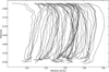 |
Fig. 7 Measured bisectors in the cross-correlated intensity line profile of Betelgeuse spectra observed from November 2013 to April 2019 with Narval at the TBL. The cross-correlation uses Mask C5 from Kravchenko et al. (2018), which selects lines forming high in the star’s photosphere. |
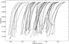 |
Fig. 8 Same as in Fig. 7, but the mask used for cross-correlation selects atomic lines with central depressions between 0.7 and 0.8 of the continuum. This filter approximately selects lines forming deep in the star’s photosphere. |
 |
Fig. 9 Bisectors computed using the image of Betelgeuse inferred to best fit the linear polarization signal observed on December 20, 2013. Parabolic gradients reducing the radial velocity are used, with various values of β as indicated. The maximum velocities at each point over the disk are reduced to 70% of the value inferred from fitting the linear polarization signal, to avoid the broadening of the profiles in the cases with small β, thus keeping the computed profiles as narrow as the ones observed. |
5 Conclusion
A bare-bones radiative transfer scheme may describe the main observed features of intensity line profiles in RSGs. The main feature addressed in this work is the currently unexplained narrowness of the observed intensity line profiles compared to the broad profiles seen in linear polarization. By stripping the radiative transfer problem of most of its complexities – particularly any variation in the absorption coefficients along the optical path or across the stellar disk – we can distill the primary factor responsible for this difference between the profiles. We find that the combination of strong velocity gradients along the line of sight, together with the brightness inhomogeneities across the stellar disk is sufficient to broaden or narrow the line profiles as needed. This can be understood with the following simplified picture: Strong velocity gradients cause the points around the disk center to contribute triangular profiles to the integrated line profile, spanning the full range of velocities but greater intensity toward redder wavelengths. Points close to the limb contribute narrow Gaussian profiles at these same red wavelengths. The result of integrating these contributions is a narrow near-Gaussian profile. A reduction in velocity gradients is enough to convert the triangular profiles emerging near the disk center into square, bottom-flat shapes that broaden the resulting profiles and possibly split the intensity line. In contrast, the linear polarization profile arises from single scattering events at the base of the line formation region, where the velocities are higher, and no further radiative transfer takes places. The wave-length position of each linear polarization signal is set deep in the line formation region, and the signal amplitude reflects the continuum brightness seen by atoms deep in the photosphere, thus probing even deeper atmospheric layers. This scenario supports the validity of the brightness – velocity relationship imposed in the inversion algorithm that produces images of Betelgeuse’s photosphere from linear polarization profiles – a relationship that holds only if convection still dominates plasma dynamics.
Using this simple radiative transfer model, together with the disk brightness distributions inferred from fitting the observed linear polarization profiles in Betelgeuse, produces intensity profiles that are remarkably analogous to the observed ones in terms of width and bisector shape. The very same model and brightness distributions can produce intensity profiles comparable to those observed in RW Cep by simply altering the velocity gradient. These two RSGs represent the extremes of intensity profile variability. Over the past 11 years, Betelgeuse has consistently shown narrow profiles, while RW Cep has shown broad intensity profiles. Both stars, moreover, exhibit similarly broad polarization profiles.
We analyzed these two RSGs in depth because they represent the two extremes of the situation under scrutiny. Previously published spectropolarimetry of µ Cep and CE Tau places these two RSGs alongside Betelgeuse, exhibiting intensity profiles that are narrower than their linear polarization profiles. Though not yet published, we can report that our observations of PZ Cas reveal broad profiles similar to those of RW Cep, thereby completing the set of RSGs observed with high-resolution spectropolarimetry.
The favorable agreement between computed and observed intensity profiles is further supported by the comparison of their line bisectors. Once again, by adjusting the velocity gradient, our simple radiative transfer model succeeds in reproducing both the C-shape (decelerating velocity gradient) and inverse C-shape (accelerating velocity gradient) of the observed bisectors. The most pronounced inverse C-shape bisectors, observed in lines forming high in the atmosphere, appear to require a change of sign of the gradient. The decrease in velocity with height that produces the C-shape bisectors must be transformed via acceleration to explain the inverse C-shape. This may be (over)interpreted as indicating that these high-forming lines originate in regions where stellar wind acceleration has already begun.
Summing up, the narrow intensity profiles of observed in Betelgeuse and the broad intensity profiles seen in RW Cep – both accompanied by similarly broad linear polarization Profiles – do not require any change in the underlying physics of these two red supergiants. Taking into account velocity gradients along the line of sight and integrating over an inhomogeneous disk is sufficient. Steep gradients explain the narrow intensity profiles of Betelgeuse, while shallow gradients explain the broad profiles of RW Cep. The hypothesis of single scattering and the correlation between velocity and brightness, which underpin the interpretation of linear polarization, are supported by our results.
If our conclusions are correct, RW Cep is presently unable to diminish the large vertical velocities of its photospheric plasma. These large velocities may help greater amounts of plasma escape gravity, and we may expect RW Cep to expel larger clouds of circumstellar matter. Betelgeuse, on the contrary, is mostly able to slow down its plasma. Moreover, its stellar wind must be dwindling. How two RSGs, largely identical in their fundamental parameters, can behave so differently remains an open question. The apparent existence of cyclical Decin stages (Decin et al. 2006; López Ariste et al. 2023) supports the idea that these steeper or shallower velocity gradients appear repeatedly during the life of an RSG.
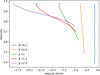 |
Fig. 10 Computation of bisectors as in Fig. 9, but using a linearly accelerating gradient. Several cases of spatial acceleration β are shown as indicated in the labels. |
Acknowledgements
This work was supported by the “Programme National de Physique Stellaire” (PNPS) of CNRS/INSU co-funded by CEA and CNES. We acknowledge support from the French National Research Agency (ANR) funded project PEPPER (ANR-20-CE31-0002).
References
- Anugu, N., Gies, D. R., Roettenbacher, R. M., et al. 2024, ApJ, 973, L5 [CrossRef] [Google Scholar]
- Aurière, M., López Ariste, A., Mathias, P., et al. 2016, A&A, 591, A119 [NASA ADS] [CrossRef] [EDP Sciences] [Google Scholar]
- Bertout, C., & Magnan, C. 1987, A&A, 183, 319 [NASA ADS] [Google Scholar]
- Chandrasekhar, S. 1945, Rev. Mod. Phys., 17, 138 [NASA ADS] [CrossRef] [Google Scholar]
- Decin, L., Hony, S., de Koter, A., et al. 2006, A&A, 456, 549 [NASA ADS] [CrossRef] [EDP Sciences] [Google Scholar]
- Donati, J.-F., Semel, M., Carter, B. D., Rees, D. E., & Collier Cameron, A. 1997, MNRAS, 291, 658 [NASA ADS] [CrossRef] [Google Scholar]
- Donati, J. F., Catala, C., Landstreet, J. D., & Petit, P. 2006, ASP Conf. Ser., 358, 362 [Google Scholar]
- Gray, D. F. 2008, AJ, 135, 1450 [Google Scholar]
- Josselin, E., & Plez, B. 2007, A&A, 469, 671 [NASA ADS] [CrossRef] [EDP Sciences] [Google Scholar]
- Kravchenko, K., Van Eck, S., Chiavassa, A., et al. 2018, A&A, 610, A29 [NASA ADS] [CrossRef] [EDP Sciences] [Google Scholar]
- Kravchenko, K., Chiavassa, A., Van Eck, S., et al. 2019, A&A, 632, A28 [NASA ADS] [CrossRef] [EDP Sciences] [Google Scholar]
- López Ariste, A., Mathias, P., Tessore, B., et al. 2018, A&A, 620, A199 [NASA ADS] [CrossRef] [EDP Sciences] [Google Scholar]
- López Ariste, A., Wavasseur, M., Mathias, P., et al. 2023, A&A, 670, A62 [NASA ADS] [CrossRef] [EDP Sciences] [Google Scholar]
- López Ariste, A., Georgiev, S., Mathias, P., et al. 2022, A&A, 661, A91 [NASA ADS] [CrossRef] [EDP Sciences] [Google Scholar]
- Wagenblast, R., Bertout, C., & Bastian, U. 1983, A&A, 120, 6 [NASA ADS] [Google Scholar]
All Figures
|
Fig. 1 Profiles of Betelgeuse observed from November 27, 2013, to March 3, 2015, with Narval at the TBL. The red vertical dashed line marks the chosen reference velocity υ∗ interpreted as the velocity of the star’s center of mass. The blue dashed line marks the maximum vertical velocity υmax of the plasma. |
| In the text | |
|
Fig. 2 Examples of profiles generated in the presence of strong gradients along the line of sight, and the resulting disk-integrated profiles. Left: profiles made in the absence of velocity gradients. The projection onto the line of sight shifts the position of the local profile. A simple limb-darkening law proportional to cos µ makes the summed profile asymmetric. Center: Employed linear velocity gradient. Right: gradient along the line of sight following a square-root law. In all cases, the same limb-darkening law as in the left panel is applied. Dashed red lines represent individual lines of sight from the disk center, θ = 45°, and close to the limb. Solid blue lines show the disk-integrated profile. Vertical dashed lines mark the radial outward velocity of the plasma, υ0 = υmax = −40 km s−1, in the observer’s frame, and the zero velocity υ∗. |
| In the text | |
|
Fig. 3 Examples of RW Cep profiles observed with NeoNarval in 2023, with dates indicated in the legend. Intensity is shown in the left plot, while Stokes Q and U are displayed in the center and right plots, respectively. The red and blue vertical dashed lines mark the chosen values of υ∗ and υmax, respectively. |
| In the text | |
|
Fig. 4 Example of local (red) and integrated (blue) profiles along the vertical radius of the image of Betelgeuse that best fit the observations of linear polarization on December 20, 2013. All profiles are normalized to the continuum value for clarity in the plot. |
| In the text | |
|
Fig. 5 Left: inferred images of Betelgeuse from November 27, 2013, to March 3, 2015, used to integrate profiles under the assumption that, at every point, the gradient is such that the velocity reduces to 0 at the top of the line formation region (β = 1). Profiles are shifted in ordinates for clarity. Right: observed intensity profiles from those same dates. |
| In the text | |
|
Fig. 6 Left: same as Fig. 5, but for β = 0.4. The maximum velocity is kept at 40 km s−1, as for Betelgeuse. Right: Observed intensity profiles of RW Cep, as in Fig. 3. The key points of comparison are the broadening of the profiles and their triangular shape, illustrated by the step-rising blue wing. |
| In the text | |
|
Fig. 7 Measured bisectors in the cross-correlated intensity line profile of Betelgeuse spectra observed from November 2013 to April 2019 with Narval at the TBL. The cross-correlation uses Mask C5 from Kravchenko et al. (2018), which selects lines forming high in the star’s photosphere. |
| In the text | |
|
Fig. 8 Same as in Fig. 7, but the mask used for cross-correlation selects atomic lines with central depressions between 0.7 and 0.8 of the continuum. This filter approximately selects lines forming deep in the star’s photosphere. |
| In the text | |
|
Fig. 9 Bisectors computed using the image of Betelgeuse inferred to best fit the linear polarization signal observed on December 20, 2013. Parabolic gradients reducing the radial velocity are used, with various values of β as indicated. The maximum velocities at each point over the disk are reduced to 70% of the value inferred from fitting the linear polarization signal, to avoid the broadening of the profiles in the cases with small β, thus keeping the computed profiles as narrow as the ones observed. |
| In the text | |
|
Fig. 10 Computation of bisectors as in Fig. 9, but using a linearly accelerating gradient. Several cases of spatial acceleration β are shown as indicated in the labels. |
| In the text | |
Current usage metrics show cumulative count of Article Views (full-text article views including HTML views, PDF and ePub downloads, according to the available data) and Abstracts Views on Vision4Press platform.
Data correspond to usage on the plateform after 2015. The current usage metrics is available 48-96 hours after online publication and is updated daily on week days.
Initial download of the metrics may take a while.