© The Authors 2025

1 Introduction

It is often not possible to determine a precise orbit for many asteroids, especially newly discovered ones, because of observational errors. Rather, there is a set of possible orbits for this asteroid, which are also often called ‘virtual asteroids’ (VAs) (Milani et al. 2000). The greater the number of these VAs that collide with the Earth, the higher the impact probability of the asteroid.

The methods for estimating the probability that an asteroid collides with the Earth can be divided into two groups: linear and nonlinear methods. Linear methods assume a linear relation between the errors of the orbital parameters at the epoch of observation and at the epoch of a possible collision. A general assumption of a Gaussian law of the errors of the orbital parameters at the epoch of observation yields a Gaussian distribution of the errors of the orbital parameters for the entire considered range of time. Linear methods are fast, they require integrating only the nominal orbit of an asteroid (the orbit that resulted from the least-squares fit of the observations) with variational equations. The uncertainty region, that is, the region of possible positions of the asteroid, is approximated with a covariance matrix.

The first linear method that was applied to the problem was the target-plane method (Chodas 1993). The approach required the nominal position of the asteroid to be close to the Earth at the time of a possible collision and ideally, that the asteroid entered its sphere of influence (approximately 2.4 lunar distances), which does not occur often. In this method, Cartesian coordinates and velocities are used as orbital parameters. The uncertainty region of an asteroid is therefore described as an ellipsoid, but in reality, this region is a thin curved line that stretches mostly along the nominal orbit. When the nominal position of an asteroid is not close to the Earth, the method is consequently unreliable and can fail.

In order to overcome this limitation of linear methods Vavilov & Medvedev (2015) proposed a method that uses an original curvilinear coordinate system with mean anomaly as one of the coordinates. This system was constructed in order to model the uncertainty region of an asteroid correctly at any time, when it is large and stretched, mostly along the nominal orbit (see Sect. 2.2.1). Later, Vavilov (2020) improved the method by introducing the concept of partial-banana mapping (PBM). The main idea of this approach is that instead of focusing on accurately approximating the whole uncertainty region, only the small part of the uncertainty region is of interest that will approach or collide with the Earth. This part is determined and mapped onto the target plane using the target plane method to estimate the impact probability. This concept is much more reliable than the classical target plane method and still requires the propagation of the nominal orbit alone, that is, it is computationally fast. However, it is still a linear method, and it therefore cannot take the fact into account that gravitational perturbations affect different parts of the uncertainty region differently, in particular, during close encounters.

The nonlinear methods lack this limitation, but require propagating at least thousands of orbits of VAs. The simplest technique is the Monte Carlo approach: Generating VAs from the probability density function at the epoch of observations and propagating their orbits. The number of VAs that collide with the Earth, divided by all considered VAs yields the impact probability. For this method, there is an explicit formula of the accuracy of the result: ${\sigma }_{MC}=\sqrt{P_{MC}(1-P_{MC})/n}$, where P_MC is the impact probability, and n is the number of considered VAs. Although it is conceptually simple, this approach has a significant limitation: The number of all considered VAs must be large enough for a sufficiently accurate probability value. Orbit integration is not a fast operation, and this makes the method time consuming and increasingly inefficient for low-impact probability values.

For a higher efficiency, a line-of-variation (LOV) sampling approach was introduced (Milani et al. 2002, 2005b,a). In general, the six-dimensional confidence ellipsoid of the orbital parameters at the epoch of observations has one main axis, and this axis is much larger than the other axes. The idea of LOV is to generate VAs on this one-dimensional main line of the confidence ellipsoid alone and to integrate the orbits of all VA to search for close encounters. By exploring these close encounters, virtual impactors can be found and the impact probability can be estimated. The LOV method is used in impact-monitoring systems of NASA (Sentry), NEODyS, and ESA (CLOMON-II). In contrast to LOV, the new version of the NASA system Sentry-II (Roa et al. 2021) consists of sampling the full confidence region and also searches for close encounters. Then, an impact pseudo-observation is introduced and an orbit-fitting procedure is applied to determine a collisional orbit that agrees with the observations. Both methods can successfully deal with deviations from the two-body formalism. They require the integration of several thousand VA orbits, however.

We present a semilinear approach for computing the impact probability. We extended the partial banana mapping method to explicitly identify the state vector within the initial confidence ellipsoid that leads to a collision. On one hand, the new approach requires the integration of several orbits, and it is therefore not as fast as linear methods, but it is still faster than nonlinear methods. On the other hand, the method is able to take the gravitational perturbations in the uncertainty region into account. The limitation of the approach is that the uncertainty region of an asteroid at the epoch of a possible collision must not be longer than the entire orbit, or that the error of the mean anomaly must not exceed 2π.

The paper is organized as follows: Section 2 presents the revision of linear methods, including the description of a special curvilinear coordinate system. Section 3 describes the new semilinear approach. In the results section, we compare the impact probabilities obtained by different methods and some discussion. This is followed by the conclusion.

2 Summary of linear methods

In order to properly explain the improvements that we introduce here, we first describe the target plane method (Kizner 1961; Greenberg et al. 1988) Sect. 2.1 and then the partial banana mapping method Sect. 2.2. The various steps for computing the collision time and orbit and the corresponding impact probability are described in Sect. 2.2.2. Keeping the same notations, we recall in this section all basic equations and properties, and we refer to the original papers (Vavilov & Medvedev 2015; Vavilov 2020) for a more detailed description.

In general, the orbit of an asteroid is derived through an orbital fitting with a least-squares method (Gauss 1809), and the errors of the obtained orbital parameters are well approximated by the Gaussian law. In linear methods, we also assume a linear relation between the errors of the orbital parameters at the epochs of observation and at the epoch of a possible collision, t. Consequently, the probability density function of the parameter errors at time t is also Gaussian.

2.1 Target plane method

Let $(x_0,y_0,z_0,\dot{x_0},\dot{y_0},\dot{z_0})$ be the state vector of an asteroid at the epoch of observations, t₀, derived through orbital fitting, and let C₀ be its variance-covariance matrix. Integrating the orbit of an asteroid with variational equations (Battin 1964) until the time at which it enters the sphere of influence of the Earth, t, provides the state vector ($x,y,z,\dot{x},\dot{y},\dot{z}$) at time t and the partial derivative matrix, $$\mathbf{\Phi }(t_0,t)=\left(\begin{array}{ccc}\frac{\mathrm{\partial }x}{\mathrm{\partial }{x}_0}& \cdots & \frac{\mathrm{\partial }x}{\mathrm{\partial }{\dot{z}}_0}\\ ⋮& \ddots & ⋮\\ \frac{\mathrm{\partial }\dot{z}}{\mathrm{\partial }{x}_0}& \cdots & \frac{\mathrm{\partial }\dot{z}}{\mathrm{\partial }{\dot{z}}_0}\end{array}\right).$$(1)

The variance-covariance matrix at time $t,{\mathbf{C}}_{xyz\dot{x}\dot{y}\dot{z}}$, is $${\mathbf{C}}_{xyz\dot{x}\dot{y}\dot{z}}=\mathbf{\Phi }(t_0,t){\mathbf{C}}_0{\mathbf{\Phi }}^{\mathrm{T}}(t_0,t),$$(2)

where T denotes the matrix transpose operation. Matrix ${\mathbf{C}}_{xyz\dot{x}\dot{y}\dot{z}}$ provides an approximation of the uncertainty region of an asteroid at time t. The velocity of an asteroid relative to the Earth is almost identical for all VAs in this area, and they therefore all move in the same direction with an almost similar speed. To estimate the impact probability, we first map this 6D uncertainty region onto the target plane, that is, the plane perpendicular to the relative velocity of the asteroid and Earth at time t. The VAs that collide with the Earth move inside a circle on the target plane that is centered at the center of Earth (see Fig. 1). Because of gravitational attraction, however, the trajectory of a VA in the sphere of influence resembles a hyperbola, and the distance between the Earth and a VA is therefore smaller than if the VA moved in a straight unperturbed direction. This distance q can be found from $$q=\frac{b}{\sqrt{1+\frac{v_s^2}{v_{\mathrm{\infty }}^2}}},$$(3)

where v_s is the escape velocity from the surface of the Earth (≈11.186 km s⁻¹), v_∞ is the unperturbed geocentric velocity, and b is the impact parameter, that is, distance on the target plane between the center of Earth and the projection of the VA.

Any VA whose distance q is smaller than the radius of the Earth, R_⊕, will collide with the Earth, or equivalently, it will collide when its impact paramter b is smaller than $R_{\oplus }\sqrt{1+\frac{v_s^2}{v_{\mathrm{\infty }}^2}}$. Therefore, to estimate the collisional probability, we can map the uncertainty region onto the target plane and then compute the probability that an asteroid is closer to the projected center of the Earth than $R_{\oplus }^{\mathrm{\prime }}=R_{\oplus }\sqrt{1+\frac{v_s^2}{v_{\mathrm{\infty }}^2}}$.

The transition from the 6D Cartesian coordinates and velocities to 2D coordinates on the target plane can be described as a multiplication by a 2 × 6 matrix, B: u = Bw. The variance-covariance matrix on the target plane reads ${\mathbf{C}}_{\mathbf{T}\mathbf{P}}={\mathbf{B}\mathbf{C}}_{xyz\dot{x}\dot{y}\dot{z}}{\mathbf{B}}^{\mathbf{T}}$ (Rao 1952). We placed the nominal asteroid in the center of the coordinate system and computed the impact probability as $$P=\frac{1}{2\pi {|\det {\mathbf{C}}_{\mathbf{T}\mathbf{P}}|}^{\frac{1}{2}}}{\int }_{S_{R_{\oplus }^{\mathrm{\prime }}}}{e}^{-\left({\mathit{u}}^{\mathrm{T}}{\mathbf{C}}_{\mathbf{T}\mathbf{P}}{}^{-1}\mathit{u}\right)/2}\mathrm{d}\mathit{u},$$(4)

where $S_{R_{\oplus }^{\mathrm{\prime }}}$ is a circle with a radius $R_{\oplus }^{\mathrm{\prime }}$.

The limitation of the applicability of the method is that the nominal VA asteroid should approach the Earth closely. This does not occur often when the impact probability is lower than 1%. Moreover, if the uncertainty region is large and curved, the target plane method is unable to detect a possible collision. Last, when the linear relation between the errors on the orbital parameters in different epochs is not fulfilled, the target plane method can only be applied when the nominal VA asteroid collides with the Earth.

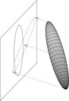Fig. 1 Schematic illustration of the target plane method. The ellipsoid represents the uncertainty region of an asteroid when it enters the sphere of influence, the plane is the target plane, the circle on the plane is the projection of the Earth, and the ellipse on the plane is the projection of the ellipsoid. Image credit: Vavilov (2018).

2.2 Partial-banana mapping method

2.2.1 Special coordinate systems

When we consider only the two-body problem (the Sun and the asteroid), then each virtual asteroid does not change its six Keplerian orbital elements with time, except for the mean anomaly. The mean anomaly is linearly related to the mean motion and time. Because of the difference in mean motions among the VAs, the positions of the VAs in space eventually occupy a thin region that mostly stretches along the nominal orbit of an asteroid.

A Gaussian law of errors of Keplerian orbital elements would successfully describe this region, but there is a problem with this approach: the analytical expression of the shape of the Earth is undefined in this parameter space (we assumed that the shape is a sphere). Another problem is that the Gaussian law implies that orbits with all the values of the parameters exist. For classical Keplerian orbital parameters, orbits with negative eccentricities do not exit. An equinoctial set of orbital elements (Broucke & Cefola 1972) removes some singularities. Nevertheless, the negative value of the semimajor axis is also outside the domain of the function. A replacement of the semimajor axis by the mean motion solves the problems with the domain, but the different sign with the nominal value of the mean motion yields a reverse motion, which is also contradictory.

Vavilov & Medvedev (2015) created a special curvilinear coordinate system ξ, η, M, related to the nominal asteroid orbit. The system is constructed as follows. First of all, we fix the osculating orbit of a small body (i.e., the five parameters of the osculating ellipse). The mean anomaly M in the osculating orbit is one of the coordinates of this system. The origin of the linear coordinates ξ, η is the point on the ellipse corresponding to M. The ξ-axis is perpendicular to the plane of the fixed ellipse along angular momentum. The axis η lies in the plane of the ellipse and completes (ξ, η, M) to orthogonal, so that η is perpendicular to the osculating velocity (see Fig. 2). On the other hand, the Gaussian law of the errors of the coordinates of the curvilinear system does not precisely describe the uncertainty region in the two-body problem, but it provides a good approximation. The choice between equinoctial orbital elements and the curvilinear system is arbitrary. By default, we use the curvilinear system.

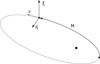Fig. 2 Curvilinear coordinate system related to the nominal orbit of an asteroid. The mean anomaly angle M is a coordinate of the system, and ξ and η are linear coordinates, the origin of which is the point corresponding to M. The vector v is the velocity of an object. Image credit: Fig. 2 in Vavilov & Medvedev (2015).

2.2.2 The algorithm

We provide the algorithm of the PBM method. Figure 3 schematically illustrates the algorithm. For a deeper understanding of the method, we refer to the original paper by Vavilov (2020).

1. Estimate the collision time: We approximate the time of the collision, t, as the time when the Earth is close to the nominal osculating orbit of the asteroid. This is calculated by numerical integration of the asteroid orbit, over a given time interval, and by computing the distance from the Earth to the osculating orbit at each time-step, selecting the local minima(s).

   Fig. 3 Schematic illustration of the confidence curvilinear ellipsoid. Point A is the nominal position of the asteroid at time t, and point B is the VA on the main axis of the confidence ellipsoid at the same time t, which is closest to the Earth after projection onto its target plane. The arrow indicates the velocity direction of Earth with respect to the confidence ellipsoid. The bold line shows the nominal orbit of the asteroid. Image credit: Fig. 3 in Vavilov (2020).

2. Integrate the orbit and calculate the covariance matrix: We integrate the asteroid orbit together with its variational equations until the estimated collision time t and obtain the variance-covariance matrix ${\mathbf{C}}_{xyz\dot{x}\dot{y}\dot{z}}$. This matrix in state-vector is transformed into curvilinear coordinates as follows: $${\mathbf{C}}_{\xi \eta M\dot{\xi }\dot{\eta }\dot{M}}=\mathbf{Q}\cdot {\mathbf{C}}_{xyz\dot{x}\dot{y}\dot{z}}\cdot {\mathbf{Q}}^{\mathrm{T}},$$(5)

   where Q is the transfer matrix, $$\mathbf{Q}=\left(\begin{array}{ccc}\frac{\mathrm{\partial }\xi }{\mathrm{\partial }x}& \cdots & \frac{\mathrm{\partial }\xi }{\mathrm{\partial }\dot{z}}\\ ⋮& \ddots & ⋮\\ \frac{\mathrm{\partial }\dot{M}}{\mathrm{\partial }x}& \cdots & \frac{\mathrm{\partial }\dot{M}}{\mathrm{\partial }\dot{z}}\end{array}\right).$$(6)

3. Spectral decomposition: We perform a spectral decomposition of ${\mathbf{C}}_{\xi \eta M\dot{\xi }\dot{\eta }\dot{M}}$, $${\mathbf{C}}_{\xi \eta M\xi \dot{\xi }\dot{M}}=\mathbf{V}\cdot \mathbf{\Lambda }\cdot {\mathbf{V}}^{\mathrm{T}},$$(7)

   where V is an orthogonal matrix of the eigenvectors, and Λ is a diagonal matrix of the eigenvalues. The principal vector corresponding to the highest eigenvalue λ₁₁ defines the main axis of the curvilinear uncertainty region.

4. Define the nominal asteroid curvilinear coordinates: We define the state vector of the nominal asteroid in curvilinear coordinates at time $t,{\mathit{w}}_t=({\xi }_t,{\eta }_t,M_t,{\dot{\xi }}_t,{\dot{\eta }}_t,{\dot{M}}_t)$, where ${\xi }_t={\eta }_t={\dot{\xi }}_t={\dot{\eta }}_t=0$.

5. Find the closest VA on the main axis: Each VA on the principal axis of the curvilinear confidence ellipsoid is found using the equation $$\mathit{u}={\mathbf{V}}^{\mathrm{T}}(\mathit{w}-{\mathit{w}}_t),$$(8)

   and setting the last five components of u to zero, that is, u = u₁, 0, 0, 0, 0, 0). With a method such as golden-section search, the value of $u_1^{\ast }$ is found, which minimizes the distance between the VA and the center of the Earth projected on the target plane (point B in Fig. 3).

6. Refine the collision time: We calculate the time correction Δt for the closest VA to cross the target plane by dividing the distance from the VA to the target plane by the relative velocity. The corrected time is t + Δt.

7. Estimate impact probability: In the vicinity of the closest VA, we approximate the uncertainty region as a segment of an ellipsoid in Cartesian coordinates. We compute the variance-covariance matrix in Cartesian coordinates for this VA, $${\mathbf{C}}_{xyz\dot{x}\dot{y}\dot{z}}^{\ast }={\mathbf{Q}}_{\ast }^{-1}\cdot {\mathbf{C}}_{\xi \eta M\dot{\xi }\dot{\eta }\dot{M}}\cdot {\mathbf{Q}}_{\ast }^{{\mathbf{T}}^{-1}}.$$(9)

   Here, Q_* is the transfer matrix, as in Eq. (6), but for the found VA (point B on Fig. 3). We calculate the impact probability P_* using the target plane method.

8. Adjust the impact probability: We correct the impact probability for the VA because it is calculated for the VA and not for the nominal asteroid. The final impact probability is eventually given by $$P={\mathrm{e}}^{-\frac{1}{2}{\left(u_1^{\ast }/\sqrt{{\lambda }_{11}}\right)}^2}{P}_{\ast },$$(10)

   where λ₁₁ is the first eigenvalue from matrix Λ.

3 PBM: Search for virtual impactors

The original PBM method is only robust when the two-body formalism can be applied. This therefore neglects all gravitational perturbations. These perturbations are sometimes not strong enough to distort the result; but there are other cases, for instance, the close approach of (99942) Apophis in 2029, where the two-body problem approximation fails. Our goal in this paper is to improve the PBM method so that it on one hand provides reliable results even with gravitational perturbations, and that on the other hand, it still works fast and does not require a large sampling of orbits to propagate.

The main idea of the method is to explicitly find the coordinates and velocities at the epoch of observations of the VA that is going to collide with the Earth in the future. This is called the virtual impactor (VI). After this, we simply use the target plane method for the VA we found and correct the resulting value by a factor that indicates the distance of the VA from the nominal solution in terms of the covariance matrix.

3.1 The main procedure

In the first stage, we proceed exactly as described above in Sect. 2.2.2 and follow the steps of the PBM method until step 5, where we find the coordinates ${\mathit{\xi }}_{\ast }=({\xi }_{\ast },{\eta }_{\ast },M_{\ast },{\dot{\xi }}_{\ast },{\dot{\eta }}_{\ast },{\dot{M}}_{\ast })$ of the VA, and step 6, where we find the corrected epoch of a possible collision t + Δt. The approximate relation between the discrepancy of the state vector at the epoch of observations, t₀, and the curvilinear coordinates at epoch t is $${\mathit{\xi }}_{\ast }-\mathit{\xi }=\left[\frac{\mathrm{\partial }\mathit{\xi }}{\mathrm{\partial }{x}_0}\right]({\mathit{x}}_{0\ast }-{\mathit{x}}_0),$$(11)

where ξ and ξ_* are the vectors in the curvilinear coordinate system of the nominal asteroid and the VA we found at time t, x₀ and x_0* are the state vectors at the epoch of observations for the nominal and that which corresponds to the VA we found. The matrix $\left[\frac{\mathrm{\partial }\xi }{\mathrm{\partial }{x}_0}\right]$ is the matrix of the partial derivatives of curvilinear coordinates at time t over the Cartesian coordinates at t₀. This matrix can be found from $$\left[\frac{\mathrm{\partial }\xi }{\mathrm{\partial }{x}_0}\right]=\mathbf{Q}\cdot \mathbf{\Phi }(t_0,t),$$(12)

where the matrix Q is the partial derivatives of the curvilinear coordinates over the Cartesian coordinates at time t (see Eq. (6)), and Φ(t₀, t) is the matrix from Eq. (1).

From Eq. (11), we therefore determine x_0*, the coordinates and velocities of the virtual asteroid, which in theory should be closest to the Earth at time t on the main line of the curvilinear uncertainty region. We take x_0*, propagate up to time t, and use the target plane method to compute the impact probability because this VA will approach Earth closely or even collide with it. This approach takes all the gravitational perturbations included in the dynamical model into account, with a cost of one additional numerical integration.

In practice, the state vector x_0* we found can be different from the vector closest to the Earth in the uncertainty region because the relation in Eq. (11) is only a linear approximation. We therefore iterate the same scheme from step 2 in Sect. 2.2.2, taking x_0* as a nominal asteroid: We compute the covariance matrix ${\mathbf{C}}_{\xi \eta M\xi \dot{\eta }\dot{M}}$, then determine the closest VA (ξ_*), and from Eq. (11) find new x_0* until the procedure converges. For better convergence, a regularization can be used; for instance, instead of taking x_0*, we can take ${\hat{\mathit{x}}}_{0\ast }={\mathit{x}}_0+k({\mathit{x}}_{0\ast }-{\mathit{x}}_0)$, where k is smaller than one.

After we determine x_0*, which corresponds to the closest VA on the main line of the uncertainty region, we verify whether it collides with the Earth approximately at time t. When the VA we found collides, we use the target plane method for this orbit and multiply the result by the factor $$\exp [-\frac{1}{2}{[{\mathit{x}}_{0\ast }-{\mathit{x}}_{\mathbf{0}}]}^{\mathrm{T}}{\mathbf{C}}_0[{\mathit{x}}_{0\ast }-{\mathit{x}}_{\mathbf{0}}]],$$(13)

which takes into account that the x_0* we found is not the nominal one. Here, C₀ is the covariance matrix at the epoch of observations in Eq. (2).

3.2 Checking for spurious collision

If the VA we found did not collide with the Earth, then this collision can be spurious. We follow the criteria from Milani et al. (2005a) that a potential collision is real only if the initial conditions leading to an impact can be found. Starting from the x_0* we found, we try to find a small change in the initial conditions that led to an impact.

The vector of Cartesian coordinates and velocities of the VA at time t can be split into two components [r, s], where r coincides with the coordinates on the target plane (2D vector) and s is a 4D vector, which basically contains the distance to the target plane and the three components of the velocity. Let C be the covariance matrix of this VA.

Our first goal was to determine the 6D state vector [r_*, s_*] at a time t of the orbit that leads to a collision and that has the highest value of the probability density function. Only vector r determines the collision with the Earth, and vector s is mapped onto the target plane. The VA we found in the previous step is closest to the Earth along the VAs on the main line of the uncertainty region. We therefore find the intersection to the projection of Earth in the directions perpendicular to the main line. This is the coordinate r_* of the vector for which we are searching.

The covariance matrix C of [r, s] at time t can be decomposed as $$\mathbf{C}=\left(\begin{array}{cc}{\mathbf{C}}_{\mathbf{r}}& {\mathbf{C}}_{\mathbf{r}\mathbf{s}}\\ {\mathbf{C}}_{\mathbf{s}\mathbf{r}}& {\mathbf{C}}_{\mathbf{s}}\end{array}\right)$$(14)

According to Milani et al. (2005a), vector s_* can be found from $${\mathbf{s}}_{\mathbf{\ast }}=\mathit{s}+{\mathbf{C}}_{\mathbf{r}}^{-1}{\mathbf{C}}_{\mathbf{s}\mathbf{r}}(\mathit{r}-{\mathit{r}}_{\mathbf{\ast }}).$$(15)

We then try to find the small change in vector x_0* at t₀ that lead to vector [r_*, s_*] at time t, and hence, to the collision. The linear relation reads $$\left[\right({\mathit{r}}_{\mathbf{\ast }},{\mathit{s}}_{\mathbf{\ast }}\left)\right]-[(\mathit{r},\mathit{s})]=\mathbf{W}\cdot \mathbf{\Phi }(t_0,t)({\tilde{\mathit{x}}}_{0\ast }-{\mathit{x}}_{0\ast }),$$(16)

where matrix W is a 6 × 6 rotation matrix leading to the coordinate system related to the target plane.

When the state vector ${\tilde{\mathit{x}}}_{0\ast }$ does not lead to a collision approximately at time t, this process needs to be iterated taking ${\tilde{\mathit{x}}}_{0\ast }$ as x_0* and using Eqs. (15) and (16). If the procedure does not determine a collision, we consider this impactor as spurious.

4 Verification

We verified the method by computing the impact probability values on the set of asteroids used in previous papers (Vavilov & Medvedev 2015; Vavilov 2020). This set of asteroids was chosen randomly from the website of the Jet Propulsion Laboratory, NASA¹, but it preferably had the highest impact probabilities. Some of the asteroids from the list were observed again in the meantime and were removed from the impact risk table. This set of asteroids can therefore be considered as modeled examples, based on real asteroids. The observational information about the asteroids is presented in Table 1. We also added asteroid 2010 RF12 and asteroid (99942) Apophis to the set, which increased the set to a total of 16 cases. For Apophis, we computed the orbit only from the observations in 2004-2006, so that it has a possible collision in 2036, that is, just after its close encounter with the Earth in 2029.

The orbits of the asteroids were computed by the method based on an exhaustive search of orbital planes (Bondarenko et al. 2014). For the orbit integration, we used the Everhart method (Everhart 1974) of 15th order. We took the gravitational attraction from major planets, Pluto, and the Moon into account, whose coordinates were obtained by the planetary ephemeris DE423 (Folkner et al. 2009).

We compared the results computed with the new semilinear approach with the linear PBM method, with the target plane method, and with a Monte Carlo method (see Table 2). We considered the results obtained with the Monte Carlo method as reference values because the method lacks any additional assumptions. The standard deviation of the Monte Carlo method results was calculated according to $\sqrt{P_{MC}(1-P_{MC})}/\sqrt{n}$, where n is the number of realizations, and P_MC is the Monte Carlo probability. We mark the values that differ from the P_MC value by more than 3σ_MC in the table in boldface. σ_MC can be arbitrarily small depending on the choice of the number of realizations, n. Regardless of the choice of n, however, the results of the new method are closer to P_MC. It should be noted that for asteroid 2010 RF12, the Monte Carlo method did not find even one collisional VA among the 972 000 VAs we considered. The likelihood that with a collision probability P_MC the Monte Carlo method finds zero collisions with n realizations is (1 − P_MC)ⁿ. To estimate 3σ_MC, we determined P_MC so that this likelihood was lower than 0.003. Subtracting n = 972 000, we find that P_MC < 5.8 · 10⁻⁶.

The comparison shows that the classical target plane method gave reliable results for only three cases. The results of the linear PBM are more reliable. For eight asteroids, it obtained adequate values, and for six more, the results did not differ by an order of magnitude. On the other hand, TP and PBM totally failed for the cases of (99942) Apophis and 2010 RF12, where there are very close encounters of these asteroids with the Earth that entirely destroy the linear relation of the errors of the orbital parameters. The new IPBM approach is consistent with the Monte Carlo method for each of the asteroids. This is logical because the new approach explicitly determined the virtual impactor. For all of these cases (except for 2010 RF12), it took only one additional orbit integration to determine the virtual impactor (no iterations). It is important to note that the most computationally demanding aspect of the method is the orbit integration. On a modern PC, this process typically takes no more than a few seconds per orbit when the integration time does not exceed 100 years into the past or future. Therefore, the proposed technique becomes twice slower than other linear methods, but still orders of magnitude faster than nonlinear methods.

Asteroid Apophis has an exceptional close encounter with the Earth in 2029, and therefore, the linear approximation for later years is not valid and the linear methods do not work. However, the new approach allowed us to successfully determine the impacting orbit, starting from the nominal one. The case for asteroid 2010 RF12 is also very interesting. This asteroid has a precise orbit, and the linear estimates of the impact probability are quite high (several percent). The close approach in 2010 during the discovery yielded nonlinearities, however, and prevents the asteroid from colliding in 2095. We confirmed that the Monte Carlo method was unable to find any collisions after we tested more than 972 000 virtual asteroids, and the approach for finding a virtual impactor had to diverge too far from the nominal solution. NASA’s nominal orbit of this object is different, and their system accordingly predicts a possible collision. The difference appears to be small, however. The ephemeris prediction for September 5, 2095, diverges by 4.34 · 10⁻⁴ au, or fewer than 10 Earth radii. For some of the other asteroids, the difference exceeds one revolution around the Sun.

It is also worth noting that instead of the curvilinear coordinate system, we tested the usage of orbital elements (both Keplerian and equinoctial) for the new approach. The results are consistent with each other in at least five digits in the mantissa with a floating point (i.e., the relative difference is smaller than 0.01%). This is logical because the idea was to explicitly determine the virtual impactor, and they therefore basically all determined the same impacting orbit and obtained the same results. Nevertheless, to compute the impact probability, the curvilinear coordinate system is preferred in order to avoid singularities with close to zero eccentricities and inclinations in classical Keplerian elements, and for a negative semimajor axis and different signs of the mean motion for equinoctial orbital elements.

We also discuss the time of the possible collision, which is a priori unknown. As a first approximation of the time of impact, we use the time when the Earth is at the closest point to the osculating nominal orbit of an asteroid, and we then correct the time. The difference between the first approximation and the actual possible collision can differ by several days, however. We decided to make the following test: We decreased the first approximation of t by 50 days. For all of the chosen asteroids (except for 2010 RF12, whose impact probability is essentially zero), the method successfully found the impacting orbit and its impact probability. It took up to five iterations, however.

The last point we discuss are the limitations of the new method. Equation (11) uses vector ξ_* in order to compute the state vector at the epoch of observations of a VA that is close to the Earth or colliding with it. We assume that the uncertainty of the mean anomaly M does not exceed 2π and that $u_1^{\ast }$ has a unique solution (see Section 2.2.2). For $u_1^{\ast }$, we always choose the closest solution to the nominal asteroid. However, if the uncertainty of the mean anomaly is large at time t, the collision can occur not for the closest solution and can be missed by the method. Since the diameter of the Earth is 8.5 · 10⁻⁵ au and the length of the asteroid orbit is several π and probably longer than 2π, when the error of M is larger than 2π, the impact probability is ≲10⁻⁵. Thus, there are no theoretical limitations for the method to determine the impact probabilities ≳10⁻⁵.

5 Conclusion

Computing and monitoring the impact probability of a near-Earth asteroid (or a potentially hazardous one) is crucial for planetary defense. This has to be performed routinely as new objects are discovered and new observations obtained. Priority can be given to objects that require additional data or to understanding the collisional risk and defining mitigation measures.

We proposed a semilinear method for estimating the impact probability. This method is an extension of the robust linear PBM method. The new approach determines explicit initial conditions in the orbital space that lead to a collision. This requires several additional numerical integrations for the orbit propagation, and the method is called semilinear for this reason. For all of the considered 16 test cases, however the method succeeded at the first try (two integrations in total) and obtained accurate impact probability values. Although it was not tested extensively on all NEOs in the current risk list, the method provided reliable results for our randomly selected test cases. This was true even for significant gravitational perturbations to the two-body problem on the path to the collision, such as close encounters (e.g., the possible collision of asteroid (99942) Apophis in 2036, for which linear methods fail). Another example justifying the advantage of the new technique is the case of asteroid 2010 RF12. Linear methods provided an impact probability of several percent, and the Monte Carlo method was unable to find even one collision after testing over 972 000 virtual asteroids within the orbital uncertainty region. The new approach determined that the initial conditions for a virtual impactor are far beyond the 5σ uncertainty ellipsoid, and the impact probability is essentially zero.

Acknowledgements

This project has received funding from the European Union’s Horizon 2020 research and innovation programme under the Marie Sklodowska-Curie grant agreement #101068341 “NEOForCE”. We would like to thank the anonymous referee for very helpful comments that significantly improved the quality and readability of the paper.

Appendix A State vectors and covariance matrices of considered asteroids

References

All Tables

All Figures

	Fig. 1 Schematic illustration of the target plane method. The ellipsoid represents the uncertainty region of an asteroid when it enters the sphere of influence, the plane is the target plane, the circle on the plane is the projection of the Earth, and the ellipse on the plane is the projection of the ellipsoid. Image credit: Vavilov (2018).
In the text

	Fig. 2 Curvilinear coordinate system related to the nominal orbit of an asteroid. The mean anomaly angle M is a coordinate of the system, and ξ and η are linear coordinates, the origin of which is the point corresponding to M. The vector v is the velocity of an object. Image credit: Fig. 2 in Vavilov & Medvedev (2015).
In the text

Fig. 3 Schematic illustration of the confidence curvilinear ellipsoid. Point A is the nominal position of the asteroid at time t, and point B is the VA on the main axis of the confidence ellipsoid at the same time t, which is closest to the Earth after projection onto its target plane. The arrow indicates the velocity direction of Earth with respect to the confidence ellipsoid. The bold line shows the nominal orbit of the asteroid. Image credit: Fig. 3 in Vavilov (2020).

In the text

References

- Battin, R. H. 1964, Astronautical Guidance, eds. R. Bracewell, C. Cherry, W. W. Harman, E. W. Herold, J. G. Linvill, S. Ramo, & J. G. Truxal (New York, San Francisco, Toronto, London: McGraw-Hill Book Company), 338 [Google Scholar]
- Bondarenko, Y. S., Vavilov, D. E., & Medvedev, Y. D. 2014, Sol. Syst. Res., 48, 212 [Google Scholar]
- Broucke, R. A., & Cefola, P. J. 1972, Celest. Mech., 5, 303 [NASA ADS] [CrossRef] [Google Scholar]
- Chodas, P. W. 1993, in BAAS, 25, 1236 [Google Scholar]
- Everhart, E. 1974, Celest. Mech., 10, 35 [NASA ADS] [CrossRef] [Google Scholar]
- Folkner, W. M., Williams, J. G., & Boggs, D. H. 2009, Interplanetary Network Progress Report, 42-178, 1 [Google Scholar]
- Gauss, K. F. 1809, Theoria motvs corporvm coelestivm in sectionibvs conicis solem ambientivm. [Google Scholar]
- Greenberg, R., Carusi, A., & Valsecchi, G. B. 1988, Icarus, 75, 1 [NASA ADS] [CrossRef] [Google Scholar]
- Kizner, W. 1961, Planet. Space Sci., 7, 125 [NASA ADS] [CrossRef] [Google Scholar]
- Milani, A., Chesley, S. R., Boattini, A., & Valsecchi, G. B. 2000, Icarus, 145, 12 [NASA ADS] [CrossRef] [Google Scholar]
- Milani, A., Chesley, S. R., Chodas, P. W., & Valsecchi, G. B. 2002, Asteroid Close Approaches: Analysis and Potential Impact Detection, 55 [Google Scholar]
- Milani, A., Chesley, S. R., Sansaturio, M. E., Tommei, G., & Valsecchi, G. B. 2005a, Icarus, 173, 362 [Google Scholar]
- Milani, A., Sansaturio, M. E., Tommei, G., Arratia, O., & Chesley, S. R. 2005b, A&A, 431, 729 [NASA ADS] [CrossRef] [EDP Sciences] [Google Scholar]
- Rao, C. R. 1952, Advanced Statistical Methods in Biometric Research (New York: John Wiley & Sons), 53 [Google Scholar]
- Roa, J., Farnocchia, D., & Chesley, S. R. 2021, AJ, 162, 277 [NASA ADS] [CrossRef] [Google Scholar]
- Vavilov, D. E. 2018, Trans. IAA RAS, 14 [Google Scholar]
- Vavilov, D. E. 2020, MNRAS, 492, 4546 [NASA ADS] [CrossRef] [Google Scholar]
- Vavilov, D. E., & Medvedev, Y. D. 2015, MNRAS, 446, 705 [NASA ADS] [CrossRef] [Google Scholar]