| Issue |
A&A
Volume 689, September 2024
|
|
|---|---|---|
| Article Number | A49 | |
| Number of page(s) | 6 | |
| Section | Celestial mechanics and astrometry | |
| DOI | https://doi.org/10.1051/0004-6361/202449830 | |
| Published online | 30 August 2024 | |
Asteroid follow-up and precovery problem: Partial banana mapping solution
1
IMCCE, Paris Observatory, CNRS, univ. PSL, Sorbonne université, univ. Lille,
77 Av. Denfert-Rochereau,
75014
Paris,
France
e-mail: This email address is being protected from spambots. You need JavaScript enabled to view it.
; This email address is being protected from spambots. You need JavaScript enabled to view it.
2
Institute of Applied Astronomy, Russian Academy of Sciences,
Kutuzova emb. 10,
St. Petersburg,
Russia
e-mail: This email address is being protected from spambots. You need JavaScript enabled to view it.
Received:
1
March
2024
Accepted:
6
June
2024
Abstract
Context. Precovery of asteroids, that is, finding older observations of already discovered asteroids, allows us to refine our knowledge of their orbits, glean information about close encounters and the probability of collisions with Earth, and to determine some dynamical and physical properties, such as the Yarkovsky acceleration. Existing approaches generally look for an observation next to the predicted position from the nominal orbit, and often do not take into account the whole uncertainty distribution of coordinates.
Aims. We aim to develop a computationally fast technique for predicting the possible spherical coordinates of near-Earth asteroids in order to find observations in existing catalogs or archived observations (plates, CCDs, etc.).
Methods. We modified the partial banana mapping method, and used it to estimate impact probabilities of asteroids with the Earth. For a near-Earth asteroid, a Gaussian law for the equinoctial orbital elements well approximates the uncertainty region of the object at the epoch of the observation. We sample virtual asteroids on the main line of the curved uncertainty region at the epoch of observation, project all of them with their small uncertainty vicinity onto the celestial sphere, and evaluate the brightness of the asteroids. We also estimate the probability of finding the asteroids on the image, and the length of the uncertainty region (which shows the quality of the orbit) in order to establish a priority list among the images. The higher the probability and the poorer the quality of the orbit, the more interesting it is to find the object for further improvement of its orbit and to refined its impact probability computation.
Results. We demonstrate the applicability of the developed method. We tested it on the case of precovery observations of asteroid (506074) Svarog (provisional designation 2015 UM67 ) as if it had recently been discovered, meaning the orbit is obtained with only 3 months of observations. In this case, we estimated a probability of precovery of about 10%, predicted the possible positions, and actually found the object close to the constructed uncertainty region. The nominal position is outside of the image’s field of view, meaning that conventional methods would fail. The uncertainty region is curved and asymmetric, which shows that using only the covariance matrix of celestial coordinates for the nominal orbit would poorly approximate the actual uncertainty region in the place of the sky, preventing the asteroid from being found.
Conclusions. The developed method selects interesting images and guides us in our search for asteroids on them, even if the position predicted for the nominal orbit is out of the image window.
Key words: methods: numerical / celestial mechanics / minor planets, asteroids: general / minor planets, asteroids: individual: (506074) Svarog
© The Authors 2024
 Open Access article, published by EDP Sciences, under the terms of the Creative Commons Attribution License (https://creativecommons.org/licenses/by/4.0), which permits unrestricted use, distribution, and reproduction in any medium, provided the original work is properly cited.
This article is published in open access under the Subscribe to Open model. This email address is being protected from spambots. You need JavaScript enabled to view it. to support open access publication.
1 Introduction
In recent years, we have witnessed some imminent impactors, that is, asteroids detected in space only several hours before they impact the Earth, and sometimes leaving several meteorites on the ground. After discovery, not only were their orbits computed by impact monitoring systems, but their impact probability rapidly increased to 100%, meaning that they were destined to enter the Earth’s atmosphere (Farnocchia et al. 2019). The alert and predicted trace on the ground allowed us to observe their atmospheric entry and perform field research to collect the meteorites. However, this situation is far from common to all newly discovered near-Earth objects (NEOs; presently approximately 3000/yr). The impact probability (IP) of such new NEOs, which is automatically computed by monitoring systems (CLOMON-2, Sentry-II, Aegis, Del Vigna et al. 2019; Roa et al. 2021; Faggioli et al. 2023), can sometimes be large enough to enter the top of the so-called risk-list catalog of all objects on a possible impact trajectory, even if it is less than 1%. Luckily, all of these recently discovered imminent impactors were small asteroids of a few meters wide, but the risk associated with larger NEOs or potentially hazardous asteroids (PHAs) can be high, even if they have a much lower impact probability upon discovery (Rumpf et al. 2017). Thus, rapid and reliable IP monitoring is an important asset to planetary defence.
For impact monitoring and IP computation of NEOs, we rely on knowledge of their orbits. A fraction of newly discovered NEOs show a non-negligible collision probability within the next century due to their proximity to the Earth’s orbit and poor knowledge of their orbit. Thus, once an object has been discovered during an apparition and observed over a short arc, follow-up observations (recovery) during the next apparition are generally necessary to refine its orbit and collision probability. As shown in Micheli et al. (2014), “precovery” observations, that is, observations made fortuitously predating the discovery, are as valuable as “recovery” ones for the computation of the orbits of these objects. In order to look for ancient observations, or plan future ones, one needs some prediction of an object’s location in the sky. We therefore need not only the position of the asteroid but also some knowledge of the uncertainty region within which to look. The same general problem applies to both follow-up and precovery. The present work focuses on precovery. These precovery observations can be processed rapidly, without the need to wait for the next apparition, which in the case of long-synodic-period bodies can take up to a decade. The objects can moreover obtain a larger observational arc, corresponding to several apparitions – which is beneficial to improvement of the orbit (Desmars et al. 2013). The discovery of asteroid (99942) Apophis in December 2004, then designated 2004 MN4, highlights the importance of planetary defence. It also serves as a good illustrates of the evolution of orbit uncertainty characterization, and the corresponding IP changes, as additional astrometric data are ingested in the orbit computation; including, in this case, beneficial precovery images taken several months before the discovery (Sansaturio & Arratia 2008, see).
Several works and programs of precovery have been undertaken since the increase in SSA and NEO risk awareness (Boattini et al. 2001; Micheli et al. 2014, 2016; Weryk & Wainscoat 2016; Saifollahi et al. 2023), often using modern CCD observations and archives accessible online, but also making use of more ancient observations from the late 19th to the 20th century, which were usually made with photographic plates, and archived at the observatories (e.g., Perlbarg 2023). However, several limitations can reduce precovery efficiency. With the progress made in current surveys, catalogue completeness are regularly pushed to smaller objects. As a consequence many objects detected presently can be too faint to be detected on ancient photographic plates. Nevertheless, some NEOs are bright enough to be seen on archived photographic plates, depending on their absolute magnitude and distance. Another limitation arises when our knowledge of the orbit of an asteroid is poor: when propagating this orbit back in time, we obtain an uncertainty region that can cover a large fraction of the sky, making the search very difficult (similarly difficult to searching for lost objects). As a consequence, precovery searches are often focused on objects with well-known orbits, or do not take into account orbital uncertainty (e.g., Perlbarg et al. 2023). Alternatively, authors filter out some regions to narrow down the search to sources that are more likely to be detectable (Saifollahi et al. 2023); thus, they can be biased toward precovery of positions close to the nominal position, that is, the position predicted from the nominal orbit; a limitation that is a consequence of not taking into account the possible large expansion of the uncertainty region and also not accounting for the velocity of the asteroid at time of observation.
In the present work, we develop a technique to better take into account the uncertainty region around the predicted position at the time of observation. This technique is based on propagation of the uncertainty of the orbit in equinoctial elements using the partial banana mapping method (PBM) (Vavilov 2020). It improves both the chance and efficiency of precovery, and is computationally fast enough to be applied to a large set of targets. The technique moreover provides the probability of finding a NEO on a given archived plate or CCD/CMOS image. In a future paper, we will demonstrate the effect of this technique on orbit improvement, determination of impact probability, and the Yarkovsky effect when such precovery astrometry is added. This orbit improvement is expected to be particularly valuable when the asteroid’s predicted nominal position is far from the observed position.
Apart from the possible low brightness of the object, another problem that we encounter when trying to find an asteroid on an old CCD or photographic plate is the uncertainty of its position. If the uncertainty is high then the asteroid can be far from the expected position and even outside of the field of view. To handle this issue, Milani et al. (2005) proposed sampling clones of the asteroid (“virtual asteroids”) along the main line of the orbital confidence region. The orbits of the virtual asteroids (VAs) should be integrated to the epoch of the interested observation. The coordinates of the VAs describe the uncertainty region of the asteroid at the epoch of the observation. This approach requires the integration of all VAs’ orbits, which increases the orbit integration and hence computation time by several orders of magnitude. However, it is more efficient than a simple Monte Carlo approach, where at least thousands of orbits of VAs must be propagated. In this study, we developed a technique that requires only integration of the nominal asteroid orbit, and can correctly approximate the uncertainty region of the asteroid’s position. We modified a linear partial banana mapping method (Vavilov 2020) the applicability of which to impact probability estimation has already been demonstrated.
The article is organized as follows. In Sect. 2, we describe our modification of the partial banana mapping method for the assigned task. In Sect. 3, we test the technique on a model example and compare it to other possible linear approaches, showing the advantages of the proposed technique. Finally, we present our conclusions in Sect. 4.
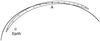 |
Fig. 1 Schematic illustration of the confidence curvilinear ellipsoid of an asteroid at time t. Point “A” is the nominal position of the asteroid, and the small black points are the virtual asteroids that we take on the main line of the confidence region at time t. The bold line is the nominal osculating orbit of the asteroid. |
2 Modification of PBM
In general, the orbit of an asteroid is derived through orbital fitting to observations using the least-squares method (Gauss 1809), and the errors of the obtained orbital parameters are well approximated by the Gaussian law. If we consider only the two-body problem (the Sun and the asteroid) then the six Keplerian orbital elements, except for mean anomaly, of each VA do not change. Furthermore, the mean anomaly is linearly related to the mean motion and time. As there is a difference in mean motion among VAs, after some time the positions of VAs in space are going to occupy a narrow region (Vavilov & Medvedev 2015) stretched mostly along the nominal orbit of an asteroid (see Fig. 1).
2.1 Uncertainty region expression
A Gaussian law of errors of the Keplerian orbital elements can approximately describe the uncertainty region mentioned in Sect. 1. However, a special approach is required to draw this uncertainty region on the celestial sphere, so that we know where to look for the asteroid in the image. Here, we modify the partial banana mapping method (Vavilov 2020) to apply the projection of the uncertainty region. Classically, the PBM method involves the use of a special curvilinear coordinate system, with the mean anomaly M being one of the coordinates. Nevertheless, for the identification problem, we decided to use an equinoctial set of orbital elements (Broucke & Cefola 1972), with the semi-major axis replaced by the mean motion. This set of orbital elements is determined by:
 (1)
(1)
where n is the mean motion, e is the eccentricity, ω is the argument of perihelion, Ω is the longitude of the ascending node, i is inclination, and M is the mean anomaly.
The negative values of eccentricities are forbidden, and so the Gaussian law of eccentricity error with a small value of eccentricity can lead to a problem. However, the equinoctial set of orbital elements does not have this singularity in the case of small eccentricities. We replaced the semi-major axis with the mean motion because of the linear relation between the mean motion and the mean anomaly, and therefore the longitude λ.
2.2 Possible position predictions
Our method entails checking whether some of the possible positions of the chosen asteroid are on the particular image at time t. Let w0 = (x0,y0,z0,ẋ0,ẏ0,ż0) be a vector of coordinates and velocities at the epoch of observations t0, and C0 be the variance-covariance matrix. Then the variance-covariance matrix at time t is:
 (2)
(2)
where T denotes the matrix transpose operation and Φ(t0, t) is a matrix of partial derivations:
 (3)
(3)
where w = (x, y, z, ẋ, ẏ, ż) is a vector of coordinates and velocities at time t. In general, this matrix is computed while integrating the equations of motion of the asteroid with the variational equations (Battin 1964).
We can express the variance-covariance matrix in equinoctial orbital elements, Cnhkλpq, as:
 (4)
(4)
where Q is the transfer matrix (partial derivatives of orbital elements over Cartesian coordinates and velocities):
 (5)
(5)
Although matrix Q can be derived numerically, the analytical way (Broucke & Cefola 1972) is more accurate and computationally faster.
Now we have an analytical approximation of the possible positions of the asteroid at time t, but it is an expression in equinoctial orbital elements (Gaussian law). In order to find the uncertainty region of the asteroid on the celestial sphere (in right ascension and declination), we could randomly choose virtual asteroids from this Gaussian law, convert each orbit to a state vector in Cartesian coordinates, and then map these onto the celestial sphere (Monte Carlo approach), but this is computationally expensive. Instead, we take only 51 VAs on the main line of the uncertainty region in the [−5σ; 5σ] interval. We consider each of the VAs as a representative of its small vicinity of the uncertainty region and map them onto the celestial sphere with their small vicinities. We do this as follows.
The covariance matrix Cnhkλpq is a positive definite matrix. Hence, we can use a spectral decomposition of this matrix:
 (6)
(6)
where V is an orthogonal matrix composed of eigenvectors of matrix Cnhkλpq and Λ is a diagonal matrix with eigenvalues on a diagonal.
Let the eigenvalue in the first row and first column be the maximal one. Let w0 = (n0, h0, k0,λ0, p0, q0,) be the equinoctial orbital elements of the nominal asteroid and w be a six-dimensional random vector in the equinoctial orbital elements. The covariance matrix of w is Cnhkλpq. Λ is a covariance matrix for the random vector u = VT(w − w0) (Rao 1952). As Λ is a diagonal matrix if the last five components of vector u equal zero (u = (u1, 0,0,0,0,0)), it defines a VA on the main axis of the six-dimensional confidence ellipsoid in orbital elements.
With a given u1, one can compute orbital elements and positions and velocities of a VA, and then map them onto the celestial sphere (getting right ascension α* and declination δ* with  ). As mentioned above, we take 51 uniformly distributed VAs, or in other words we sample u1 uniformly in the interval [
 ], where Λ11 is the component of matrix Λ in the first row and first column, and is also the largest one.
For a given VA, we first correct its position for aberration. As the speed of light, c, is limited, we observe the position of the object not at time t, but slightly before, at t − Δt, which is found from
 (7)
(7)
where rE(t − Δt) is the distance between the observatory and the asteroid at t − Δt and c is the speed of light.
We then map the small uncertainty area around the VA as follows. Let (x*,y*,z*,ẋ*,ẏ*,ż*) and (n*h*k*λ*p*q*) be the Cartesian state vector and equinoctial orbital elements of the found VA, respectively. First, we shrink the uncertainty region along the main axis by 50 times (because we decided to take 51 VAs). This is done by dividing Λ11 by 502, yielding matrix Λ*. The matrix that expresses the small uncertainty region around this VA (in orbital elements) is
 (8)
(8)
However, this shrunken region is much shorter, and its curvature is not significant. Therefore, we then compute the covariance matrix for this VA in Cartesian coordinates. The transfer matrix is
 (9)
(9)
The covariance matrix in Cartesian coordinates and velocities corresponding to the chosen VA is given by
 (10)
(10)
The covariance matrix in right ascension and declination of the VA is obtained from
![Mathematical equation: ${\bf{C}}_{\alpha \delta \dot \alpha \dot \delta }^* = {\left[ {{{\partial \alpha } \over {\partial x}}} \right]^*} \cdot {\bf{C}}_{xyz\dot x\dot y\dot z}^* \cdot {\left[ {{{\partial \alpha } \over {\partial x}}} \right]^{*{\rm{T}}}},$](/articles/aa/full_html/2024/09/aa49830-24/aa49830-24-eq13.png) (11)
(11)
where ![Mathematical equation: ${\left[ {{{\partial \alpha } \over {\partial x}}} \right]^*}$](/articles/aa/full_html/2024/09/aa49830-24/aa49830-24-eq14.png) is the matrix of partial derivatives of right ascension, declination and their velocities over Cartesian coordinates and velocities for the chosen VA.
is the matrix of partial derivatives of right ascension, declination and their velocities over Cartesian coordinates and velocities for the chosen VA.
We follow the steps described above for each VA (for each value of u1), thus obtaining the spherical coordinates and the uncertainty region of all VAs. These data show us the possible position in the sky of the asteroid at the time of the image (CCD or photographic plate). We mark the VAs, the coordinates of which are inside the image boundaries, in order to gauge the possibility that this asteroid can be found on this image.
For each of the VAs, the estimated apparent magnitude is computed using the following equation:
 (12)
(12)
where H is the absolute magnitude of the asteroid, r is the asteroid heliocentric distance, and rE is the distance between the observatory and the asteroid. The last term in Eq. (12) is related to the dimming of the asteroid from the nonzero Sun-asteroid-observatory angle, γ (Bowell et al. 1989). We use the following version of the function:
![Mathematical equation: $\Phi (\gamma ) = (1 - G)\exp \left[ { - {A_1}{{(\tan (\gamma /2))}^{{B_1}}}} \right] + G\exp \left[ { - {A_2}{{(\tan (\gamma /2))}^{{B_2}}}} \right].$](/articles/aa/full_html/2024/09/aa49830-24/aa49830-24-eq16.png) (13)
(13)
The coefficients are A1 = 3.332, A2 = 1.862, B1 = 0.631, and B2 = 1.218, and G is the slope parameter, which is generally assumed to be 0.15.
2.3 Prioritizing the images
As well as computing the possible positions of each Near-Earth object for all available photographic plates and CCDs, we also computed the length of the main line of the uncertainty region on the celestial sphere. This length shows the accuracy of our prediction of the asteroid ephemeris. For instance, if the length is less than 1 arcsec, the accuracy of the ephemeris is probably better than the accuracy of this observation. On the other hand, if the length is thousands of arcseconds or more, then this observation can significantly improve the accuracy of the calculated orbit.
The second important term is the probability that the asteroid is located inside the image boundaries. We estimate this value using the following equation:
 (14)
(14)
where the set  is the sampling of u1 for the chosen VAs in terms of
  (meaning they take values from −5 to +5 with a step of 0.2), and Θ(xi) is equal to 1 if the VA corresponding to xi is on the image and 0 otherwise. We normalize this by dividing the sum by ten. Thus, it is an approximation of the Gaussian integral.
We this method to search for known near-Earth asteroids on old photographic plates available at the Paris observatory. Scanning the image and looking for an asteroid takes up to 1 h, and therefore we need to prioritize the plates on which we ran this procedure. First, we eliminate all the asteroids that are estimated to be fainter than 19m or 20m on the images. The rest we sort by the probability value and the length of the uncertainty region. The higher the probability, the greater the chance of successful precovery. Also, the larger the uncertainty region, the more valuable the observation will be for improving the orbit and potentially determining the Yarkovsky effect. Finally, the asteroids that are in an impact risk table, such as NASA Sentry1, are given high priority, even if the probability of finding them is below that of other asteroids that are not on an impact risk table.
 |
Fig. 2 Possible positions of asteroid (506074) Svarog on 06:00:00 1 March 1990 on the orbit constructed from observations made during the first 3 months following its discovery. The purple box is the photographic plate. The orange dot is the nominal position. The blue dots are the 50 virtual asteroids, and the lines connecting them are the uncertainty regions of each VA (they are very narrow). The red dot is the actual observation. The green line is the uncertainty region of the nominal position constructed from only the covariance matrix in right ascension and declination. |
3 Test
In order to test this technique based on PBM, we performed the following experiment. We chose asteroid (506074) Svarog (2015 UM67), which was discovered on 28 October 2015 by MASTER-SAAO observatory and was the subject of 195 observations up to 15 January 2016. For almost a year (until 23 December 2016), no observations of this asteroid were carried out. Here we decided to check whether or not it would be possible to find this object on the photographic plates available at the Paris observatory, in an imaginary scenario where subsequent observations were unavailable (e.g., if the asteroid got lost, or if this analysis were being carried out in 2016).
We chose this asteroid because we already knew it had been detected on a photographic plate of the Palomar observatory dated 06:00:00 on 1 March 1990 (Perlbarg 2023). The 5σ ephemeris uncertainty at this epoch for the orbit derived from the entire set of observations is only 27 arcsec. However, for the orbit derived from only the first 3 months of data following the discovery, the uncertainty length is 74 134 arcsec, making it more difficult to detect.
Figure 2 shows the possible positions of this asteroid on that date if the orbit is constructed from observations in the first 3 months following its discovery (blue dots). The nominal ephemeris position (orange dot) is outside of the plate (purple box), making it impossible to find the object using a more classical approach based only on the position of the nominal without taking into account the uncertainty region (Perlbarg et al. 2023). The red dot is the actual observation. The probability of finding the asteroid on this plate was estimated to be around 10%.
We note that the region of possible positions (blue dots) is curved and asymmetric, as expected. The figure also shows the uncertainty region computed by taking the covariance matrix in right ascension and declination for the nominal position (green line). This latter is symmetric and straight, because it follows the equation of an ellipsoid in spherical coordinates. Using only this will give us inaccurate information and may prevent us from finding the object, especially if the real uncertainty region is more curved. It should also be noted that the most computationally expensive procedure is the integration of the orbit from the epoch of observations to the plate epoch, and therefore calculating 51 positions of VAs is almost as fast as drawing the uncertainty region from the covariance matrix.
Figure 3 presents a zoom onto the observation presented in Fig. 2. The red line is the observation found by Perlbarg et al. (2023). The observation has the appearance of a line because the photographic plate has an exposure time of 50 min. The blue dots and thin blue ellipsoids around them predict the beginning of the observation. The green thin part of the ellipsoid is as before the uncertainty region of the nominal position constructed from only the covariance matrix. The light-blue lines starting from the blue dots predict the direction and the length of the observation.
We note that the length and the direction of the observational trail were predicted accurately. There is a small discrepancy between the start of the observational trail and the prediction; there are two possible sources of this difference. The first is related to the fact that the technique still assumes a linear relation between the errors of the orbital elements at the epoch of observations and the plate epoch. It correctly approximates the uncertainty region in the two-body formalism, but gravitational perturbations from major planets can violate the linear relation and distort the region. In any case, the accuracy of this PBM prediction is much higher than that made by the covariance matrix of the nominal solution with similar CPU time. The second possible source of the above discrepancy is the timing of the plates, which is sometimes imprecise. This discrepancy due to timing error can be adjusted during the orbit fitting by including this in the error model in the astrometry position along the apparent motion (Perlbarg et al. 2023).
It took approximately 0.359 s to compute these results for asteroid Svarog on a PC with a 12th Gen Intel(R) Core(TM) i7-12700H 2.30 GHz processor. This demonstrates that our method is an efficient technique for asteroid follow-up and precovery. We compared our method with a simple Monte Carlo approach, whereby at the epoch of observations, several virtual asteroids are randomly taken from the uncertainty region according to the probability distribution function, their orbits are propagated until the time of the photographic plate, and then spherical coordinates for each VA are obtained. In order to properly cover a 3σ uncertainty region, one needs to use at least 1000 virtual asteroids. This approach also allowed us to successfully find the observation, however it took approximately 109.51 s (which is 305 times longer). This computation speed difference becomes crucial for a search for NEOs in a large set of images. The approach of Milani et al. (2005) would be approximately 51 times slower than the proposed technique if one were to consider the same number of virtual asteroids.
It should be noted that the proposed technique is “linear”, meaning that it can fail if an asteroid has a complex dynamical behavior; for example, with close approaches with planets between the observed arc and the possible precovery epoch. For these kinds of objects, nonlinear methods, such as a Monte Carlo, are required.
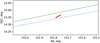 |
Fig. 3 Zoom onto the observation shown in Fig. 2. The red line is the observation found by Perlbarg et al. (2023). The observation has the appearance of a line, because the photographic plate has an exposure time of 50 min. The blue dots and thin blue ellipsoids around them predict the beginning of the actual observation. The green thin part of the ellipsoid is as before the uncertainty region of the nominal position constructed from only the covariance matrix. The light-blue lines starting from the blue dots predict the direction and the length of the actual observation. |
4 Conclusion
Precovery of asteroids, that is, finding old observations of already discovered asteroids, is an important technique for improving the orbit of an object, refining the information about its close encounters and impact probability with the Earth, and determining its physical properties, such as the Yarkovsky acceleration.
In this paper, we present a new approach to searching for possible precoveries and follow-up. We modified the Partial Banana Mapping method in which we approximate the uncertainty region of an asteroid at the time of an observation as a Gaussian law of equinoctial orbital elements. We take 51 virtual asteroids on the 5σ segment of the main line of the uncertainty region and map them onto the celestial sphere. We compute the small uncertainty of each of the virtual asteroids as well. The coordinates of virtual asteroids approximate the possible positions of the asteroid at the epoch of the observation. If all these positions are outside of the field of view, the asteroid cannot be in this CCD or photographic plate.
For each of the known near-Earth asteroids, we computed the probability that the asteroid is in the CCD, as well as the length of the uncertainty region and the expected visual magnitude. With these values, we rank the CCD and plates so that the computed probability is high but the uncertainty region is not excessively small and the object is sufficiently bright to be seen in the image. If the uncertainty region for an asteroid is relatively small, any precovery observation will not significantly improve its orbit.
We tested the developed algorithm on an example asteroid, (506074) Svarog (2015 UM67). We constructed the orbit of the asteroid using only observations from the first 3 months following its discovery. Using our method, we computed a possible 10% probability of precovery of the asteroid on the photographic plate of 1 March 1990, on which the asteroid was indeed found. We stress that the nominal position of the asteroid is outside of the plate, and so conventional approaches, such as that used by Perlbarg et al. (2023) and Saifollahi et al. (2023), would not have led to a successful precovery. This example also demonstrates that the covariance matrix for a nominal position cannot properly simulate the uncertainty region. Comparison with the Monte Carlo approach shows that our method is 300 times faster, which is important when looking for precoveries of a set of asteroids in large databases, or using large data-mining approaches.
Acknowledgements
This project has received funding from the European Union’s Horizon 2020 research and innovation programme under the Marie Sklodowska-Curie grant agreement #101068341 “NEOForCE”.
References
- Battin, R. H. 1964, Astronautical Guidance, eds. R. Bracewell, C. Cherry, W. W. Harman, E. W. Herold, J. G. Linvill, S. Ramo, & J. G. Truxal (New York, San Francisco, Toronto, London: McGraw-Hill Book Company), 338 [Google Scholar]
- Boattini, A., D’Abramo, G., Forti, G., & Gal, R. 2001, A&A, 375, 293 [NASA ADS] [CrossRef] [EDP Sciences] [Google Scholar]
- Bowell, E., Hapke, B., Domingue, D., et al. 1989, in Asteroids II, eds. R. P. Binzel, T. Gehrels, & M. S. Matthews, 524 [Google Scholar]
- Broucke, R. A., & Cefola, P. J. 1972, Celest. Mech., 5, 303 [NASA ADS] [CrossRef] [Google Scholar]
- Del Vigna, A., Milani, A., Spoto, F., Chessa, A., & Valsecchi, G. B. 2019, Icarus, 321, 647 [NASA ADS] [CrossRef] [Google Scholar]
- Desmars, J., Bancelin, D., Hestroffer, D., & Thuillot, W. 2013, A&A, 554, A32 [NASA ADS] [CrossRef] [EDP Sciences] [Google Scholar]
- Faggioli, L., Fenucci, M., Gianotto, F., et al. 2023, in 2nd NEO and Debris Detection Conference, 73 [Google Scholar]
- Farnocchia, D., Chesley, S. R., Chodas, P. W., et al. 2019, in AAS/Division of Dynamical Astronomy Meeting, 51, 200.04 [Google Scholar]
- Gauss, K. F. 1809, Theoria motvs corporvm coelestivm in sectionibvs conicis solem ambientivm, eds. F. Perthes, & I. H. Besser (Hambvrgi, Svmtibvs) [Google Scholar]
- Micheli, M., Koschny, D., Hainaut, O., & Bernardi, F. 2014, in Asteroids, Comets, Meteors 2014, eds. K. Muinonen, A. Penttilä, M. Granvik, et al. 353 [Google Scholar]
- Micheli, M., Koschny, D., Drolshagen, G., Perozzi, E., & Borgia, B. 2016, in Asteroids: New Observations, New Models, 318, eds. S. R. Chesley, A. Morbidelli, R. Jedicke, & D. Farnocchia, 274 [Google Scholar]
- Milani, A., Sansaturio, M. E., Tommei, G., Arratia, O., & Chesley, S. R. 2005, A&A, 431, 729 [NASA ADS] [CrossRef] [EDP Sciences] [Google Scholar]
- Perlbarg, A.-C. 2023, PhD thesis, Univ. PSL, Paris observatory, Paris, France [Google Scholar]
- Perlbarg, A. C., Desmars, J., Robert, V., & Hestroffer, D. 2023, A&A, 680, A41 [NASA ADS] [CrossRef] [EDP Sciences] [Google Scholar]
- Rao, C. R. 1952, Advanced Statistical Methods in Biometric Research (New York: John Wiley & Sons), 53 [Google Scholar]
- Roa, J., Farnocchia, D., & Chesley, S. R. 2021, AJ, 162, 277 [NASA ADS] [CrossRef] [Google Scholar]
- Rumpf, C. M., Lewis, H. G., & Atkinson, P. M. 2017, maps, 52, 1082 [NASA ADS] [Google Scholar]
- Saifollahi, T., Verdoes Kleijn, G., Williams, O. R., et al. 2023, in 2nd NEO and Debris Detection Conference, 29 [Google Scholar]
- Sansaturio, M. E., & Arratia, O. 2008, Earth Moon Planets, 102, 425 [NASA ADS] [CrossRef] [Google Scholar]
- Vavilov, D. E. 2020, MNRAS, 492, 4546 [NASA ADS] [CrossRef] [Google Scholar]
- Vavilov, D. E., & Medvedev, Y. D. 2015, MNRAS, 446, 705 [NASA ADS] [CrossRef] [Google Scholar]
- Weryk, R. J., & Wainscoat, R. J. 2016, in AAS/Division for Planetary Sciences Meeting Abstracts, 48, 405.03 [NASA ADS] [Google Scholar]
All Figures
|
Fig. 1 Schematic illustration of the confidence curvilinear ellipsoid of an asteroid at time t. Point “A” is the nominal position of the asteroid, and the small black points are the virtual asteroids that we take on the main line of the confidence region at time t. The bold line is the nominal osculating orbit of the asteroid. |
| In the text | |
|
Fig. 2 Possible positions of asteroid (506074) Svarog on 06:00:00 1 March 1990 on the orbit constructed from observations made during the first 3 months following its discovery. The purple box is the photographic plate. The orange dot is the nominal position. The blue dots are the 50 virtual asteroids, and the lines connecting them are the uncertainty regions of each VA (they are very narrow). The red dot is the actual observation. The green line is the uncertainty region of the nominal position constructed from only the covariance matrix in right ascension and declination. |
| In the text | |
|
Fig. 3 Zoom onto the observation shown in Fig. 2. The red line is the observation found by Perlbarg et al. (2023). The observation has the appearance of a line, because the photographic plate has an exposure time of 50 min. The blue dots and thin blue ellipsoids around them predict the beginning of the actual observation. The green thin part of the ellipsoid is as before the uncertainty region of the nominal position constructed from only the covariance matrix. The light-blue lines starting from the blue dots predict the direction and the length of the actual observation. |
| In the text | |
Current usage metrics show cumulative count of Article Views (full-text article views including HTML views, PDF and ePub downloads, according to the available data) and Abstracts Views on Vision4Press platform.
Data correspond to usage on the plateform after 2015. The current usage metrics is available 48-96 hours after online publication and is updated daily on week days.
Initial download of the metrics may take a while.