| Issue |
A&A
Volume 698, June 2025
|
|
|---|---|---|
| Article Number | A316 | |
| Number of page(s) | 8 | |
| Section | The Sun and the Heliosphere | |
| DOI | https://doi.org/10.1051/0004-6361/202554363 | |
| Published online | 24 June 2025 | |
Dependence of the intensity of the non-wave component of extreme UV waves on the coronal magnetic field configuration
1
Key Laboratory of Modern Astronomy and Astrophysics, School of Astronomy and Space Science, Nanjing University, Nanjing 210023, PR China
2
State Key Laboratory of Lunar and Planetary Sciences, Macau University of Science and Technology, Macau 999078, PR China
⋆ Corresponding author: This email address is being protected from spambots. You need JavaScript enabled to view it.
Received:
4
March
2025
Accepted:
13
May
2025
Abstract
Mounting evidence has shown that extreme-ultraviolet (EUV) waves consist of a fast-mode magnetohydrodynamic (MHD) wave (or shock wave) followed by a slower non-wave component, as predicted by the magnetic field line stretching model. However, not all observed events display both wave fronts, particularly the slower non-wave component. Even when the slower non-wave component is present, the intensity distribution often exhibits strong anisotropy. This study is intended to unveil the formation condition of the slower non-wave component of EUV waves. We analyzed the EUV wave event on 8 March 2019 and compared the EUV wave intensity map with the extrapolation coronal potential magnetic field. Data-inspired MHD simulation was also performed. Two types of EUV waves are identified, and the slower non-wave component exhibits strong anisotropy. By reconstructing 3D coronal magnetic fields, we find that the slower non-wave component of EUV waves is more pronounced in regions where magnetic fields are backward-inclined, which is further reproduced by our MHD simulations. The anisotropy of the slower non-wave component of EUV waves is strongly related to the magnetic configuration, with backward-inclined field lines favoring their appearance. The more the field lines are forward-inclined, the weaker such wavelike fronts become.
Key words: Sun: activity / Sun: corona / Sun: coronal mass ejections (CMEs) / Sun: magnetic fields
© The Authors 2025
 Open Access article, published by EDP Sciences, under the terms of the Creative Commons Attribution License (https://creativecommons.org/licenses/by/4.0), which permits unrestricted use, distribution, and reproduction in any medium, provided the original work is properly cited.
This article is published in open access under the Subscribe to Open model. This email address is being protected from spambots. You need JavaScript enabled to view it. to support open access publication.
1. Introduction
Solar extreme-ultraviolet (EUV) waves are a spectacular and frequently observed large-scale wave phenomenon associated with other solar eruptions, such as solar flares, filament eruptions, and coronal mass ejections (CMEs; Moses et al. 1997; Thompson et al. 1998; Chen 2006; Nitta et al. 2013; Mei et al. 2020). Initially, since EUV waves often propagate in a quasi-isotropic manner (Moses et al. 1997; Thompson et al. 1998) and are occasionally co-spatial with Hα Moreton waves (Thompson et al. 2000; Pohjolainen et al. 2001), they were naturally considered to be fast-mode magnetohydrodynamic (MHD) waves or shock waves (Thompson et al. 1998, 1999; Wang 2000; Wu et al. 2001; Ofman & Thompson 2002). However, later studies performed by Delannée & Aulanier (1999) and Delannée (2000) discovered that EUV wave fronts sometimes stop at magnetic separatrices. In addition, EUV wave speeds are typically three times lower than those of Moreton waves (Klassen et al. 2000; Zhang et al. 2011) and can sometimes fall below 100 km s−1 (Zhukov et al. 2009; Grechnev et al. 2022), i.e., at speeds slower than coronal sound speed. All these features posed a big challenge to the fast-mode MHD wave model accounting for coronal EUV waves (Wills-Davey & Attrill 2009).
To resolve the discrepancies, Chen et al. (2002) performed MHD numerical simulations and found that, as a flux rope erupts, two EUV waves appear, i.e., a faster one and a slower one, the latter of which is immediately followed by expanding dimmings. The faster one is a fast-mode MHD shock wave piston-driven by the erupting flux rope, and the slower one is about three times slower than the faster one. To account for the formation of the slower-component EUV wave, the authors proposed the magnetic field line stretching model, an apparent propagation (the so-called “non-wave”) formed by the successive stretching of magnetic field lines pushed by the erupting flux rope. With a concentric semicircular magnetic configuration, they derived an analytical solution for the slow-component EUV wave, which is exactly about three times slower than the fast-mode wave speed. Such a feature is consistent with the statistical results (Klassen et al. 2000; Zhang et al. 2011). The prediction of two different types of EUV waves by Chen et al. (2002) was soon after confirmed by Harra & Sterling (2003) with the Transition Region And Coronal Explorer (TRACE) observations. After the high-cadence observations of the Solar Dynamics Observatory (SDO) were available, further research supported the two-wave paradigm (Chen & Wu 2011; Schrijver et al. 2011; Asai et al. 2012; Cheng et al. 2012; Kumar et al. 2013; Chandra et al. 2024; Hu et al. 2024). In fact, even before the SDO era, there was already kinematical evidence for different classes of EUV waves (Warmuth & Mann 2011), and only one class could be considered as fast-mode MHD waves (Temmer et al. 2011; Veronig et al. 2011; Patsourakos & Vourlidas 2012; Kwon et al. 2013; Selwa et al. 2013; Mann et al. 2023). It is now widely recognized that the EUV waves are composed of two components, including a fast MHD wave followed by a slower non-wave component, with the slower wave front historically referred to as the “EIT waves” (Chen et al. 2016). Although the magnetic field line stretching model is widely accepted, other interpretations for the slower non-wave component also exist, including the current shell model (Delannée et al. 2008), successive magnetic reconnection (Attrill et al. 2007), and the echo of the fast-mode shock (Wang et al. 2009; Xie et al. 2019).
Despite this fact, not all solar eruptions manifest the simultaneous existence of both components, i.e., the leading fast-mode MHD wave (or shock wave) and the subsequent non-wave. For example, during the SOlar and Heliospheric Observatory (SOHO) era, only the slower non-wave component could be detected in most events, which was due to the low cadence of its EUV telescope. According to Chen & Wu (2011), only when the observational cadence was less than ∼70 s, could the fast component be detected. However, even when the cadence was as short as 12 s in the SDO data, a single wave was discernible in some events. For example, in the event studied by Zheng et al. (2020), only a single wave was observed to propagate with a speed of 500 km s−1, which would correspond to the fast-component EUV wave according to the criteria proposed in Chen et al. (2016). In contrast, the slower events in Nitta et al. (2013) with speeds below 300 km s−1 probably represent the non-wave component of EUV waves, only because the fast component is too faint. Moreover, even when the two components are visible in a single event, each wave generally exhibits strong intensity anisotropy. For the anisotropy of fast-component EUV wave fronts, it has been demonstrated that they are generally brighter near areas with a weaker magnetic field. This is due to two effects. First, a filament, once triggered to erupt, tends to propagate toward the direction with a weaker magnetic field. Such an inclined eruption further strengthens the piston-driven shock wave on the side with the weaker magnetic field (Zheng et al. 2023). Second, fast-mode MHD waves or shock waves tend to be refracted toward the area with weaker magnetic field (Uchida 1968; Liu et al. 2018; Zhou et al. 2024). It is still unclear what is responsible for the anisotropy of the slow-component EUV waves.
In this paper, we analyze an EUV wave event driven by a filament eruption on 8 March 2019, wherein the intensity of the slow-component EUV wave exhibits strong anisotropy. By performing coronal magnetic field extrapolation and MHD simulations, we investigate the relationship between the intensity distribution of EUV waves and the local coronal magnetic field configuration with the purpose to reveal the formation condition of the slow-component EUV waves. The overview of observations is described in Section 2, the coronal magnetic field reconstruction is shown in Section 3, the simulation validation ispresented in Section 4, followed by a summary and discussions in Section 5.
2. Observations and data analysis
2.1. Instruments and event overview
The event under study is a filament eruption associated with a C1.3-class flare on 8 March 2019 in NOAA active region (AR) 12734. Although the flare was very weak, this filament eruption excited distinct bright wave fronts. The filament eruption produced a CME and was accompanied by a type II radio burst, which is a typical CME-driven EUV wave event. This event was well documented by the Atmospheric Imaging Assembly (AIA) on board the SDO satellite (Lemen et al. 2012). The AIA instrument has seven EUV channels and provides solar full-disk images with a spatial resolution of 0.6″ per pixel and a temporal cadence of 12 s. Typically, due to significant density compression at the EUV wave front, the wave front is clearer in the 193 Å difference images. Therefore, in this study, we primarily selected the 193 Å channel for observation. To better track the propagation of the EUV wave, we extracted slices along different directions on the solar surface and considered the spherical projection effect, starting from the eruption source site. Furthermore, to reduce uncertainties in the observations, we set a certain width for each slice in each direction, which allowed for a more accurate tracing of the EUV wave front motion (Shen & Liu 2012).
2.2. Observations of EUV waves
Figure 1 displays running-difference images in the 193 Å channel, in which each image is processed with the Gaussian smoothing technique with a full width at half maximum being 3 pixels to reduce noises. This eruption produces two wavelike fronts, including a leading weak front (the red line in Figure 1b) and an ensuing wave with patchy fronts (the green lines in Figure 1b) followed by dimmings. The leading wave, with a roughly elliptic shape, is rather isotropic as indicated by the dashed red line in Figure 1b. The ensuing wave is more anisotropic, being extremely bright in the southwest direction, and marginally visible in the north direction, but nearly invisible in the south direction, as indicated by the dashed green line in Figure 1b.
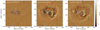 |
Fig. 1. SDO/AIA 193 Å running-difference images illustrating the evolution of the EUV wave on 8 March 2019. The base time is 24 s earlier for each panel. The dashed red and green lines represent the two-component wave fronts in panel b. The animation of this figure is available online. |
To quantitatively investigate the kinematics of the EUV waves, we selected three slices (the green lines in Figure 2a) to generate time-distance diagrams, as shown in Figures 2b–2d. The oblique green and blue lines outline the wave fronts propagating along each slice. In Figure 2b, the first wave front appears around 03:10 UT along the southwest direction of slice S1, with a speed of 420 ± 60 km s−1. Subsequently, a second wave front is observed around 03:16 UT followed by dimmings. It propagates at a slower speed of 170 ± 15 km s−1 initially; soon after, it stops, appearing as a patchy EUV wave as investigated by Guo et al. (2015). Figure 2c shows the results of slice S2 in the south direction, where a wave can be identified to propagate with a speed of 380 ± 20 km s−1. Additionally, at a distance of 250″, a stationary front is observed, as discovered by Chandra et al. (2016). Such a feature was attributed to mode conversion from fast-mode wave to slow-mode wave, which is trapped at magnetic separatrix (Chen et al. 2016; Chandra et al. 2018; Kumar et al. 2024). Along the northward slice S3, Figure 2d shows two wave patterns. The first wave propagates out rapidly with a speed of 620 ± 30 km s−1, starting from around 03:09 UT. The other wave, which immediately borders the extending dimmings, propagates more slowly and gradually decelerates, with an average speed of 210 ± 10 km s−1. Comparing Figures 2b–d, the fast-component EUV wave appears marginally isotropic, being slightly strongest in the southwest direction. In contrast, the slow-component EUV wave is much more anisotropic, being most pronounced in the southwest direction and the weakest in the south direction.
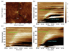 |
Fig. 2. Time-distance diagrams of the base-difference intensity at EUV 193 Å channel along slices S1 (southwest, panel b), S2 (south, panel c), and S3 (north, panel d). The slice trajectories are marked in panel a. Two wave fronts and the fitting speeds are shown in panels b and d, while only one wave is visible in panel c. Note that both the fast MHD wave component (green lines) and the slower non-wave component (cyan lines), accompanied by pronounced expanding dimmings, are visible along slices S1 and S3, whereas only the fast MHD wave component can be clearly identified along slice S2. The error bars are estimated from the upper and lower boundaries of wave fronts. |
3. Relationship between 3D coronal magnetic fields and EUV waves
It is expected that the properties of EUV waves are highly dependent on the coronal magnetic fields. Therefore, to explain the anisotropy of EUV waves in the spatial distribution, we reconstruct 3D coronal magnetic fields with the potential field extrapolation in the spherical coordinate achieved by the method in PDFI_SS library (Fisher et al. 2020). The computation domain extends from the solar surface to 2 solar radii, where the source surface is located.
Figures 3a–b show the 3D coronal magnetic field lines from two perspectives. To investigate the relationship between the intensity of the slow-component EUV wave and the magnetic configuration, we define the exterior angle θ between a magnetic field line and the solar surface at the footpoint as follows:
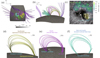 |
Fig. 3. Panels a–b: Top view and side view of the 3D coronal magnetic field reconstructed with the potential-field extrapolation; panel c: Distribution of the exterior angle (color scale) overlaid on the SDO/AIA 193 Å map at 03:15:04 UT; panels d–f: Selected field lines, indicating those field lines traced from the western (yellow) and northern (magenta) regions. These are more backward inclined compared to those from the eastern (cyan) and southern (green) regions. |
 (1)
(1)
where Br is the radial component of the vector magnetogram and Bt is the transverse component. With this definition, the magnetic field line is forward inclined when θ < 90°, or backward inclined when θ > 90°. We compute the exterior angle distribution of coronal magnetic fields with respect to the solar-surface plane in Figure 3c, which is overlaid on the SDO/AIA 193 Å image at 03:15:04 UT. As shown, the exterior angle of the magnetic field lines, θ, is larger than 90° near the strongest patch of the slow-component EUV wave in the southwest direction. It is less than but close to 90° in the north direction where the slow-component EUV wave is moderate. In contrast, θ is significantly smaller in the south direction, where the slow-component EUV wave is nearly invisible. This means that the intensity of the slow-component EUV wave becomes greater as the exterior angle of the field line at the footpoint increases.
Based on the above analysis along with the 3D coronal magnetic-field extrapolation, we find that the intensity of the slow-component EUV waves is strongly related to coronal magnetic fields and is brighter at the backward-inclined magnetic field lines (e.g., the southwest direction in Figure 3c). In the case of a forward-inclined magnetic configuration, the more inclined the field line is, the weaker the slow-component EUV wave (e.g., the south and north directions in Figure 3c). Selected magnetic field lines in the southwest, north, and south directions are displayed in Figures 3d–f.
4. Data-inspired MHD simulation
4.1. Numerical setup
To validate the above conclusion extracted from observations and magnetic-field modelings, we conducted a 3D data-inspired MHD simulation to investigate how different configurations of background magnetic fields affect the intensity of slow-component EUV waves. To this end, we constructed the initial magnetic-field configuration with different exterior angles of the background magnetic field lines on the two sides of a magnetic flux rope. Based on Titov-Demoulin-modified model (Titov et al. 2014) (but slightly different from the original case with two magnetic charges), the initial background magnetic fields are provided by four sub-photosphere magnetic charges (q1 = 10 × 1020 G cm2, q2 = −10 × 1020 G cm2, q3 = 1.3 × 10²⁰ G cm2, and q4 = −1.3 × 10²⁰ G cm2), placed at the positions of (10, 0, −10), (−10, 0, −10), (120, 0, −100), and (−10, 0, −100) Mm, respectively. The former two charges represent the fields of the core AR, while the latter two charges are adopted to imitate the large-scale magnetic fields. Then, a stable and force-free toroidal-shaped flux rope is inserted with the regularized Biot-Savart laws (Titov et al. 2018) with a peak height of 10 Mm. In particular, to ensure that the initial magnetic-field system is stable, we used the magneto-frictional method (Guo et al. 2016) to relax it to a force-free state. The relaxed magnetic-field configuration is shown in Figure 4a, from which it is clear that the field lines on the right side are more vertical (or even backward-inclined) compared to those on the left (which are forward-inclined). Consequently, the exterior angle of the field lines on the right side is significantly larger than that on the left.
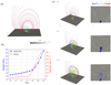 |
Fig. 4. Kinematics and 3D magnetic-field evolution of the eruption. Panel a shows the magnetic field configuration at the initial state. The yellow, cyan, and red-wine lines represent the preeruptive flux-rope field lines, the overlying active-region fields that are mainly generated by q1 and q2, and the large-scale background field lines extending from q3 and q4, respectively. Panel b shows the kinetics of the solar eruption, wherein the blue and red lines represent the evolution of the flux-rope axis height and velocity, respectively. Panel c illustrates the evolution of the 3D coronal magnetic fields and the Jy distribution in the x–z plane at t = 3τ0, 11τ0, and 13τ0. The animation of this figure is available online. |
The governing equations of our simulation are as follows:
 (2)
(2)
 (3)
(3)
 (4)
(4)
 (5)
(5)
where ρ, v, B, p, eint = p/(γ − 1), and g = −g0ez represent the density, velocity, magnetic fields, thermal pressure, internal energy, and gravity, respectively. In particular, we also adopted a uniform resistivity, η = 2.0 × 10⁻⁴ (normalized unit), for joule heating. Regarding the initial density and pressure, we adopted an isothermal atmosphere with a temperature of 1 MK, so that the density could be computed from the hydrostatic condition. The simulation includes two stages. First, to realize the energy balance, we relaxed the initial atmosphere coupled with magnetic fields until the density was almost constant. Then, to trigger the solar eruption, following Liu et al. (2024), we implemented a converging flow (the maximum velocity is 15 km s−1) on magnetic charges q1 and q2, thereby inducing magnetic reconnection below the flux rope and leading to eruption. This simulation was established on the MPI-AMRVAC framework (Xia et al. 2018; Keppens et al. 2023).
4.2. Simulation results
Figure 4 exhibits the kinematics (panel b) of the flux rope and the evolution of the 3D magnetic fields and electric current (panel c) in the eruption process. As shown in Figure 4b, the flux rope begins to rise with a velocity of about 30 km s−1 when the converging flow is imposed. This induces a quasi-static phase of the flux rope. When the flux rope slowly ascends to a height of 80 Mm at t = 6τ0 (where τ0 = 85.87 s is the normalization time), the velocity increases to about 130 km s−1, during which a hyperbolic flux tube is formed that triggers the slow rise phase of the flux rope (Xing et al. 2024). Soon after, when the current sheet became thin enough, fast reconnection was induced, triggering the start of the impulsive phase (Jiang et al. 2021), as well as the formation of a CME and certain overlying magnetic fields (cyan lines) that became part of the CME flux rope.
Figure 5 shows the evolution of the plasma temperature and density in the eruption process. Figures 5a–c illustrate the temperature distribution in the x–z plane at t = 9τ0, 11τ0, and 13τ0, respectively. A dome-like area is heated to 10 MK due to Joule heating around the cavity, corresponding to the boundary of the flux rope. In front, a moderately heated region can be seen (∼2 MK), which is due to plasma compression and is relevant to the stretching of field lines (Chen et al. 2002). Figures 5d–f show the density evolution, which clearly displays a low-density cavity in the middle and two wavelike density-enhanced fronts further out, corresponding to the dark cavity, the CME leading front, and the shock wave in the CME observations (Chen 2009; Guo et al. 2023). To investigate the kinematics of the wave fronts, we cut a slice in the x-direction at the height of 30 Mm (slice S in Figure 5f). The time-distance diagram is displayed in Figure 5g, where we can see two wave fronts propagating in both directions. Along the right direction, i.e., x > 0, a slow-component wave, indicated by the dashed green line, propagates with a speed of 53 km s−1. Such a wave pattern is immediately followed by expanding dimmings. At t = ∼8τ0, the impulsive acceleration of the flux rope drives a fast-mode shock wave, propagating outward with a speed of 195 km s−1, as indicated by the dashed red line. The speed of the slower non-wave component is ∼3.68 times lower than that of the fast-component wave. These results are highly consistent with the prediction of the field-line stretching model (Chen et al. 2002). Nevertheless, for the simplicity of numerical simulation, the magnetic field is assumed to be weak, so that the speeds of both waves are near the lower limits observed. Toward the left direction, at x < 0, we can also identify two waves, which are significantly weaker than those in the right direction.
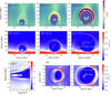 |
Fig. 5. Evolution of the plasma temperature and density during the eruption. Panels a–c show the distribution of the temperature in the x–z plane at t = 9τ0, 11τ0, and 13τ0, respectively. Panels d–f exhibit the evolution of the density in the x–z plane at t = 9τ0, 11τ0, and 13τ0, respectively. Panel g illustrates the time-distance diagram of the density along slice S in panel f. Panel h shows the distribution of the density in the x–y plane at the height of 150 Mm. The animation of this figure is available online. |
The time-distance diagram reveals that the wave fronts in the simulation exhibit strong anisotropy due to the difference in the overlying magnetic fields. To clarify this, we display the density distribution in the x–y plane at z = 150 Mm, where it can be seen that both wave fronts are stronger on the right side compared to their counterparts on the left side. Thus, our simulation results are highly consistent with the findings from observations and coronal magnetic-field extrapolations.
5. Discussions and conclusion
Waves in the solar corona not only carry energy (Russell & Stackhouse 2013), but also serve as probes to diagnose coronal information that cannot be measured directly, (e.g., magnetic field and temperature) (Ballai 2007; West et al. 2011; Long et al. 2013; Piantschitsch et al. 2018; Downs et al. 2021; Nakariakov et al. 2024). In this sense, EUV waves are particularly useful to observe, since they generally consist of a leading fast-mode MHD wave and a subsequently slower non-wave component, with the latter commonly termed an “EIT wave”. On the one hand, compared to local standing waves trapped in coronal loops or propagating waves in open flux tubes, large-scale EUV waves occupy an indispensable status in diagnosing global coronal magnetic fields. On the other hand, while the fast-component EUV waves tell us the strength of coronal magnetic fields, the slow-component EUV waves reveal the coronal magnetic topology, including magnetic geometry and separatrixes (Chen 2009; Chen et al. 2016). As such, a comprehensive understanding of the nature and formation conditions of EUV waves is a prerequisite for their application in coronal seismology.
The two-wave paradigm of EUV waves is consistent with the theoretical prediction of the magnetic field-line stretching model (Chen et al. 2002), which states that, during the eruption of a magnetic flux rope, a fast-mode piston-driven shock wave propagates as the outermost front. Behind this shock wave, a slowly propagating disturbance is generated by the ongoing stretching of magnetic field lines pushed by the flux rope. For each magnetic field line, the stretching propagates from the top part to the footpoints, compressing the plasma on the outer side of the field line to form emission enhancement, and the successive stretching of the filed lines creates an apparent wave phenomenon, i.e., “EIT waves”. It has been noted that such stretching would naturally generate a current layer (Wongwaitayakornkul et al. 2019) and sub-Alfvénic propagation of magnetic reconfiguration (Pascoe et al. 2017). Under the assumption of a concentric semicircular magnetic field configuration, the slow-component wave speed is about one third of that of the leading fast-mode wave. However in real observations, the wave phenomena are often more complicated than the canonical paradigm, presumably due to inhomogeneities in coronal magnetic fields and plasma. For example, not all events exhibit both wave components, i.e., some events only comprise the fast component (e.g., Koukras et al. 2020; Hou et al. 2023), whereas others only comprise the non-wave component. In addition, even when both components are detectable, their intensity may exhibit anisotropy. Hence, it is challenging to determine what is responsible for the anisotropy of EUV waves and, as an extreme case, why one component is missing in some events or along certain directions. For this purpose, we investigated the EUV waves associated with a CME on 8 March 2019. In this eruptive event, we observed both components of EUV waves, with the slow-component EUV wave displaying pronounced anisotropy.
The slow-component wave, or “EIT wave”, is extremely bright in the southwest direction from the source AR, moderate in the north, and much weaker in other directions, as illustrated by Figure 1. We examined the extrapolated coronal magnetic fields and compared the difference in the magnetic field at various locations. We found that the magnetic field lines around the bright “EIT wave” are more backward-inclined as indicated by Figures 3b–c, whereas the field lines in the north and south directions are forward inclined, as seen fromFigures 3e–f. Such a correlation is expected from the magnetic field-line stretching model (Chen et al. 2002). According to this model, the slow-component EUV wave is generated as the closed field lines overlying the erupting flux rope are pushed upward and stretched. The stretching of the closed field lines is associated with two motions: upward motion during the eruption and lateral motion during the expansion. When the leg of the closed field line is more backward-inclined, as illustrated by the left panel of Figure 6, both motions compress the outer plasma straightforwardly. On the other hand, when the leg of the closed field line is more forward-inclined, as illustrated by the right panel of Figure 6, the lateral motion of the field line compresses the outer plasma; however, the upward motion contracts the field line and reduces the lateral expansion. As a result, the plasma outside the field line is weakly compressed, and the EUV intensity becomes weak. Interestingly, although the slow-component EUV wave is weak in the north and south, there is still significant difference between the two directions. The slow-component wave is slightly stronger in the north than in the south direction. We checked the magnetic field inclination angles and found that, although the field lines in the two directions are both forward-inclined, the inclination angle of the field lines in the south direction is smaller, i.e., the field lines in the south direction are more inclined. Such a subtle difference further validates the paradigm presented in Figure 6. If the field line is extremely forward-inclined, no slow-component EUV wave is expected to appear.
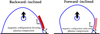 |
Fig. 6. Schematic sketch illustrating why the backward-inclined magnetic field lines yield strong plasma compression (left panel) and forward-inclined magnetic field lines result in weak plasma compression (right panel). Blue lines indicate magnetic field lines; θ denotes the exterior angle of the field lines; the dark red front represents a brighter non-wave component front; and the light red front indicates a faint non-wave component front. |
In order to confirm our explanation, we performed data-inspired MHD modeling, where several magnetic sources with opposite polarities were imposed below the simulation domain in order to generate magnetic field lines that are more forward-inclined on one side of the source AR and more backward-inclined on the other. The simulation results display several interesting features comparable with the observations. First, two EUV waves, i.e., a faster wave component and a slower non-wave component, can be clearly identified, which is similar to our previous 3D MHD simulations (Guo et al. 2023). Second, in the data-inspired simulations, the magnetic field lines to the west of the source AR are more backward-inclined, and the associated slow-component EUV waves are more intense. In contrast, the magnetic field lines to the east of the source AR are more forward-inclined, and the corresponding slow-component EUV waves are much weaker. This means that our data-inspired MHD modeling successfully reproduced the correlation between the intensity of the slow-component EUV waves and the exterior angle of the local magnetic field lines.
To summarize, observations of the 8 March 2019 flare and CME event indicate that the event was associated with two types of EUV waves: one of which is faster and the other slower. While the fast-component EUV wave is marginally isotropic, the slow-component EUV wave is strongly anisotropic, being extremely bright in the southwest direction, moderate in the north, and much weaker in other directions. We observed a strong correlation between the brightness of the slow-component EUV wave and the magnetic field configuration. To account for this a correlation, we proposed a model within the framework of the magnetic field-line stretching model: The visibility of the slow-component EUV wave depends on the exterior angle of the magnetic field lines overlying the source eruption region. The slow-component EUV wave is brighter if the leg of the magnetic field line is backward-inclined, and it is weaker if the leg of the magnetic field line is forward-inclined. The more forward-inclined the field line is, the weaker the slow-component EUV wave. The data-inspired MHD simulations further validate such a paradigm.
Our results provide a scenario for using EUV waves to diagnose coronal magnetic fields. For the slower, non-wave component of the EUV wave, its intensity is strongly related to the field-line configuration, i.e., it is more visible at places with backward-inclined magnetic field lines. With the automated detection of EUV wave features (Ireland et al. 2019; Xu et al. 2020), it is worthwhile to quantify the relationship between the intensity of EUV waves and their magnetic fields, so as to establish the basis for EUV wave seismology.
Data availability
Movies associated to Figs. 1, 4, and 5 are available at https://www.aanda.org
Acknowledgments
This research was supported by the National Key Research and Development Program of China (2020YFC2201200), NSFC (12127901) and the fellowship of China National Postdoctoral Program for Innovative Talents under grant No. BX20240159. We acknowledge the use of data from SDO. The numerical calculations in this paper were performed in the cluster system of the High Performance Computing Center (HPCC) of Nanjing University.
References
- Asai, A., Ishii, T. T., Isobe, H., et al. 2012, ApJ, 745, L18 [NASA ADS] [CrossRef] [Google Scholar]
- Attrill, G. D. R., Harra, L. K., van Driel-Gesztelyi, L., & Démoulin, P. 2007, ApJ, 656, L101 [NASA ADS] [CrossRef] [Google Scholar]
- Ballai, I. 2007, Sol. Phys., 246, 177 [Google Scholar]
- Chandra, R., Chen, P. F., Fulara, A., Srivastava, A. K., & Uddin, W. 2016, ApJ, 822, 106 [NASA ADS] [CrossRef] [Google Scholar]
- Chandra, R., Chen, P. F., Joshi, R., Joshi, B., & Schmieder, B. 2018, ApJ, 863, 101 [Google Scholar]
- Chandra, R., Chen, P. F., & Devi, P. 2024, ApJ, 971, 53 [NASA ADS] [CrossRef] [Google Scholar]
- Chen, P. F. 2006, ApJ, 641, L153 [NASA ADS] [CrossRef] [Google Scholar]
- Chen, P. F. 2009, ApJ, 698, L112 [NASA ADS] [CrossRef] [Google Scholar]
- Chen, P. F., & Wu, Y. 2011, ApJ, 732, L20 [Google Scholar]
- Chen, P. F., Wu, S. T., Shibata, K., & Fang, C. 2002, ApJ, 572, L99 [Google Scholar]
- Chen, P. F., Fang, C., Chandra, R., & Srivastava, A. K. 2016, Sol. Phys., 291, 3195 [NASA ADS] [CrossRef] [Google Scholar]
- Cheng, X., Zhang, J., Olmedo, O., et al. 2012, ApJ, 745, L5 [Google Scholar]
- Delannée, C. 2000, ApJ, 545, 512 [Google Scholar]
- Delannée, C., & Aulanier, G. 1999, Sol. Phys., 190, 107 [Google Scholar]
- Delannée, C., Török, T., Aulanier, G., & Hochedez, J. F. 2008, Sol. Phys., 247, 123 [CrossRef] [Google Scholar]
- Downs, C., Warmuth, A., Long, D. M., et al. 2021, ApJ, 911, 118 [CrossRef] [Google Scholar]
- Fisher, G. H., Kazachenko, M. D., Welsch, B. T., et al. 2020, ApJS, 248, 2 [NASA ADS] [CrossRef] [Google Scholar]
- Grechnev, V. V., Kiselev, V. I., & Uralov, A. M. 2022, Sol. Phys., 297, 106 [Google Scholar]
- Guo, Y., Ding, M. D., & Chen, P. F. 2015, ApJS, 219, 36 [Google Scholar]
- Guo, Y., Xia, C., Keppens, R., & Valori, G. 2016, ApJ, 828, 82 [NASA ADS] [CrossRef] [Google Scholar]
- Guo, J. H., Ni, Y. W., Zhong, Z., et al. 2023, ApJS, 266, 3 [NASA ADS] [CrossRef] [Google Scholar]
- Harra, L. K., & Sterling, A. C. 2003, ApJ, 587, 429 [NASA ADS] [CrossRef] [Google Scholar]
- Hou, Z., Tian, H., Su, W., et al. 2023, ApJ, 953, 171 [NASA ADS] [CrossRef] [Google Scholar]
- Hu, H., Zhu, B., Liu, Y. D., et al. 2024, ApJ, 976, 9 [Google Scholar]
- Ireland, J., Inglis, A. R., Shih, A. Y., et al. 2019, Sol. Phys., 294, 158 [Google Scholar]
- Jiang, C., Feng, X., Liu, R., et al. 2021, Nat. Astron., 5, 1126 [NASA ADS] [CrossRef] [Google Scholar]
- Keppens, R., Popescu Braileanu, B., Zhou, Y., et al. 2023, A&A, 673, A66 [NASA ADS] [CrossRef] [EDP Sciences] [Google Scholar]
- Klassen, A., Aurass, H., Mann, G., & Thompson, B. J. 2000, A&AS, 141, 357 [NASA ADS] [CrossRef] [EDP Sciences] [Google Scholar]
- Koukras, A., Marqué, C., Downs, C., & Dolla, L. 2020, A&A, 644, A90 [NASA ADS] [CrossRef] [EDP Sciences] [Google Scholar]
- Kumar, P., Cho, K. S., Chen, P. F., Bong, S. C., & Park, S.-H. 2013, Sol. Phys., 282, 523 [NASA ADS] [CrossRef] [Google Scholar]
- Kumar, P., Nakariakov, V. M., Karpen, J. T., & Cho, K.-S. 2024, Nat. Commun., 15, 2667 [NASA ADS] [CrossRef] [Google Scholar]
- Kwon, R.-Y., Ofman, L., Olmedo, O., et al. 2013, ApJ, 766, 55 [NASA ADS] [CrossRef] [Google Scholar]
- Lemen, J. R., Title, A. M., Akin, D. J., et al. 2012, Sol. Phys., 275, 17 [Google Scholar]
- Liu, W., Jin, M., Downs, C., et al. 2018, ApJ, 864, L24 [Google Scholar]
- Liu, Q., Jiang, C., Bian, X., et al. 2024, MNRAS, 529, 761 [Google Scholar]
- Long, D. M., Williams, D. R., Régnier, S., & Harra, L. K. 2013, Sol. Phys., 288, 567 [Google Scholar]
- Mann, G., Warmuth, A., & Önel, H. 2023, A&A, 675, A129 [NASA ADS] [CrossRef] [EDP Sciences] [Google Scholar]
- Mei, Z. X., Keppens, R., Cai, Q. W., et al. 2020, MNRAS, 493, 4816 [NASA ADS] [CrossRef] [Google Scholar]
- Moses, D., Clette, F., Delaboudinière, J. P., et al. 1997, Sol. Phys., 175, 571 [NASA ADS] [CrossRef] [Google Scholar]
- Nakariakov, V. M., Zhong, S., Kolotkov, D. Y., et al. 2024, Rev. Mod. Plasma Phys., 8, 19 [NASA ADS] [CrossRef] [Google Scholar]
- Nitta, N. V., Schrijver, C. J., Title, A. M., & Liu, W. 2013, ApJ, 776, 58 [Google Scholar]
- Ofman, L., & Thompson, B. J. 2002, ApJ, 574, 440 [Google Scholar]
- Pascoe, D. J., Russell, A. J. B., Anfinogentov, S. A., et al. 2017, A&A, 607, A8 [NASA ADS] [CrossRef] [EDP Sciences] [Google Scholar]
- Patsourakos, S., & Vourlidas, A. 2012, Sol. Phys., 281, 187 [NASA ADS] [Google Scholar]
- Piantschitsch, I., Vršnak, B., Hanslmeier, A., et al. 2018, ApJ, 857, 130 [Google Scholar]
- Pohjolainen, S., Maia, D., Pick, M., et al. 2001, ApJ, 556, 421 [Google Scholar]
- Russell, A. J. B., & Stackhouse, D. J. 2013, A&A, 558, A76 [NASA ADS] [CrossRef] [EDP Sciences] [Google Scholar]
- Schrijver, C. J., Aulanier, G., Title, A. M., Pariat, E., & Delannée, C. 2011, ApJ, 738, 167 [NASA ADS] [CrossRef] [Google Scholar]
- Selwa, M., Poedts, S., & DeVore, C. R. 2013, Sol. Phys., 284, 515 [Google Scholar]
- Shen, Y., & Liu, Y. 2012, ApJ, 752, L23 [NASA ADS] [CrossRef] [Google Scholar]
- Temmer, M., Veronig, A. M., Gopalswamy, N., & Yashiro, S. 2011, Sol. Phys., 273, 421 [NASA ADS] [CrossRef] [Google Scholar]
- Thompson, B. J., Plunkett, S. P., Gurman, J. B., et al. 1998, Geophys. Res. Lett., 25, 2465 [Google Scholar]
- Thompson, B. J., Gurman, J. B., Neupert, W. M., et al. 1999, ApJ, 517, L151 [Google Scholar]
- Thompson, B. J., Reynolds, B., Aurass, H., et al. 2000, Sol. Phys., 193, 161 [Google Scholar]
- Titov, V. S., Török, T., Mikic, Z., & Linker, J. A. 2014, ApJ, 790, 163 [NASA ADS] [CrossRef] [Google Scholar]
- Titov, V. S., Downs, C., Mikić, Z., et al. 2018, ApJ, 852, L21 [NASA ADS] [CrossRef] [Google Scholar]
- Uchida, Y. 1968, Sol. Phys., 4, 30 [NASA ADS] [CrossRef] [Google Scholar]
- Veronig, A. M., Gömöry, P., Kienreich, I. W., et al. 2011, ApJ, 743, L10 [Google Scholar]
- Wang, Y. M. 2000, ApJ, 543, L89 [Google Scholar]
- Wang, H., Shen, C., & Lin, J. 2009, ApJ, 700, 1716 [NASA ADS] [CrossRef] [Google Scholar]
- Warmuth, A., & Mann, G. 2011, A&A, 532, A151 [NASA ADS] [CrossRef] [EDP Sciences] [Google Scholar]
- West, M. J., Zhukov, A. N., Dolla, L., & Rodriguez, L. 2011, ApJ, 730, 122 [Google Scholar]
- Wills-Davey, M. J., & Attrill, G. D. R. 2009, Space Sci. Rev., 149, 325 [NASA ADS] [CrossRef] [Google Scholar]
- Wongwaitayakornkul, P., Haw, M. A., Li, H., & Bellan, P. M. 2019, ApJ, 874, 137 [Google Scholar]
- Wu, S. T., Zheng, H., Wang, S., et al. 2001, J. Geophys. Res., 106, 25089 [Google Scholar]
- Xia, C., Teunissen, J., El Mellah, I., Chané, E., & Keppens, R. 2018, ApJS, 234, 30 [Google Scholar]
- Xie, X., Mei, Z., Huang, M., et al. 2019, MNRAS, 490, 2918 [Google Scholar]
- Xing, C., Aulanier, G., Cheng, X., Xia, C., & Ding, M. 2024, ApJ, 966, 70 [Google Scholar]
- Xu, L., Liu, S., Yan, Y., & Zhang, W. 2020, Sol. Phys., 295, 44 [Google Scholar]
- Zhang, Y., Kitai, R., Narukage, N., et al. 2011, PASJ, 63, 685 [Google Scholar]
- Zheng, R., Chen, Y., Wang, B., & Song, H. 2020, ApJ, 894, 139 [NASA ADS] [CrossRef] [Google Scholar]
- Zheng, R., Liu, Y., Liu, W., et al. 2023, ApJ, 949, L8 [Google Scholar]
- Zhou, X., Shen, Y., Yuan, D., et al. 2024, Nat. Commun., 15, 3281 [NASA ADS] [CrossRef] [Google Scholar]
- Zhukov, A. N., Rodriguez, L., & de Patoul, J. 2009, Sol. Phys., 259, 73 [NASA ADS] [CrossRef] [Google Scholar]
All Figures
|
Fig. 1. SDO/AIA 193 Å running-difference images illustrating the evolution of the EUV wave on 8 March 2019. The base time is 24 s earlier for each panel. The dashed red and green lines represent the two-component wave fronts in panel b. The animation of this figure is available online. |
| In the text | |
|
Fig. 2. Time-distance diagrams of the base-difference intensity at EUV 193 Å channel along slices S1 (southwest, panel b), S2 (south, panel c), and S3 (north, panel d). The slice trajectories are marked in panel a. Two wave fronts and the fitting speeds are shown in panels b and d, while only one wave is visible in panel c. Note that both the fast MHD wave component (green lines) and the slower non-wave component (cyan lines), accompanied by pronounced expanding dimmings, are visible along slices S1 and S3, whereas only the fast MHD wave component can be clearly identified along slice S2. The error bars are estimated from the upper and lower boundaries of wave fronts. |
| In the text | |
|
Fig. 3. Panels a–b: Top view and side view of the 3D coronal magnetic field reconstructed with the potential-field extrapolation; panel c: Distribution of the exterior angle (color scale) overlaid on the SDO/AIA 193 Å map at 03:15:04 UT; panels d–f: Selected field lines, indicating those field lines traced from the western (yellow) and northern (magenta) regions. These are more backward inclined compared to those from the eastern (cyan) and southern (green) regions. |
| In the text | |
|
Fig. 4. Kinematics and 3D magnetic-field evolution of the eruption. Panel a shows the magnetic field configuration at the initial state. The yellow, cyan, and red-wine lines represent the preeruptive flux-rope field lines, the overlying active-region fields that are mainly generated by q1 and q2, and the large-scale background field lines extending from q3 and q4, respectively. Panel b shows the kinetics of the solar eruption, wherein the blue and red lines represent the evolution of the flux-rope axis height and velocity, respectively. Panel c illustrates the evolution of the 3D coronal magnetic fields and the Jy distribution in the x–z plane at t = 3τ0, 11τ0, and 13τ0. The animation of this figure is available online. |
| In the text | |
|
Fig. 5. Evolution of the plasma temperature and density during the eruption. Panels a–c show the distribution of the temperature in the x–z plane at t = 9τ0, 11τ0, and 13τ0, respectively. Panels d–f exhibit the evolution of the density in the x–z plane at t = 9τ0, 11τ0, and 13τ0, respectively. Panel g illustrates the time-distance diagram of the density along slice S in panel f. Panel h shows the distribution of the density in the x–y plane at the height of 150 Mm. The animation of this figure is available online. |
| In the text | |
|
Fig. 6. Schematic sketch illustrating why the backward-inclined magnetic field lines yield strong plasma compression (left panel) and forward-inclined magnetic field lines result in weak plasma compression (right panel). Blue lines indicate magnetic field lines; θ denotes the exterior angle of the field lines; the dark red front represents a brighter non-wave component front; and the light red front indicates a faint non-wave component front. |
| In the text | |
Current usage metrics show cumulative count of Article Views (full-text article views including HTML views, PDF and ePub downloads, according to the available data) and Abstracts Views on Vision4Press platform.
Data correspond to usage on the plateform after 2015. The current usage metrics is available 48-96 hours after online publication and is updated daily on week days.
Initial download of the metrics may take a while.