| Issue |
A&A
Volume 698, June 2025
|
|
|---|---|---|
| Article Number | A97 | |
| Number of page(s) | 21 | |
| Section | Stellar structure and evolution | |
| DOI | https://doi.org/10.1051/0004-6361/202553783 | |
| Published online | 03 June 2025 | |
Versatile light curve templates of Cepheids
Multi-band fitting of photometric time series
1
LIRA, Observatoire de Paris, Université PSL, Sorbonne Université, Université Paris Cité, CY Cergy Paris Université, CNRS, 5 place Jules Janssen, 92195 Meudon, France
2
French-Chilean Laboratory for Astronomy, IRL 3386, CNRS and U. de Chile, Casilla 36-D, Santiago, Chile
3
European Southern Observatory, Karl-Schwarzschild-Straße 2, 85748 Garching, Germany
4
Nicolaus Copernicus Astronomical Center, Polish Academy of Sciences, Bartycka 18, 00-716 Warszawa, Poland
5
Université Côte d’Azur, Observatoire de la Côte d’Azur, CNRS, Laboratoire Lagrange, Nice, France
6
Instituto de Alta Investigación, Universidad de Tarapacá, Casilla 7D, Arica, Chile
⋆ Corresponding author: This email address is being protected from spambots. You need JavaScript enabled to view it.
Received:
16
January
2025
Accepted:
27
March
2025
Abstract
Context. To use the period–luminosity relations of Cepheids to derive distances of extragalactic Cepheids, it is crucial to have reliable estimations of the luminosity of such stars. However, the light curves (LCs) of extragalactic Cepheids are sparsely sampled, which makes the interpolation difficult.
Aims. Our purpose is to create general templates of Cepheid LCs that can be efficiently applied with only a few parameters, while ensuring they are reliable in terms of resulting mean magnitudes. We have also aimed to provide adaptable templates for the large variety of photometric bands to enlarge their possible applications.
Methods. We performed a principal component analysis (PCA) on LCs in different bands from the optical to the mid-infrared (MIR) fitted by atmosphere models along the pulsation cycle for 75 galactic Cepheids. All the photometric bands were treated together to incorporate the results of the effective temperature variation. To link the different shapes of LCs, we also derived the relations between the period and the coefficients associated to the PCA.
Results. We present our templates and a further analysis to validate their reliability. We also offer an example of their application to one Cepheid in the galaxy NGC 5584. We find a good agreement with previous estimations of mean magnitudes in the HST filters. We show examples of a template fitting for Cepheids in various environments to demonstrate the variety of applications of these templates.
Conclusions. The templates we propose here can be used in a number of different situations (good phase coverage in many filters, poor phase coverage in one specific filter, but good phase coverage in some others, or noisy and sparse data), thereby mobilising the adapted fitting strategies. Moreover, the broad adaptability of this LC prediction tool is provided by the multiple photometric bands in which they can be inferred.
Key words: methods: data analysis / techniques: photometric / stars: distances / stars: variables: Cepheids / distance scale
© The Authors 2025
 Open Access article, published by EDP Sciences, under the terms of the Creative Commons Attribution License (https://creativecommons.org/licenses/by/4.0), which permits unrestricted use, distribution, and reproduction in any medium, provided the original work is properly cited.
This article is published in open access under the Subscribe to Open model. This email address is being protected from spambots. You need JavaScript enabled to view it. to support open access publication.
1. Introduction
Determining distances is one of the key interrogations across the field of astrophysics. For this purpose, a large variety of approaches and indicators are available, which depend on the order of magnitude of the distance. However, a lot of distance measurements rely on the so-called global distance ladder. This ladder consists of achieving distances to observable galaxies by stepping through different calibrations of various indicators (see e.g. Gaia Collaboration 2023; Pietrzyński et al. 2019; Reid et al. 2019; Leavitt & Pickering 1912; Phillips 1993, for trigonometric parallaxes, eclipsing binaries, mega-maser, Cepheids, and Type Ia Supernovae, SNIa, respectively).
This paper is focussed on multi-band light curve (LC) templates for the determinations of periods and mean magnitudes of Cepheids. When they are in other galaxies, such stars are observed e.g., using image series from theHubble Space Telescope (HST) and the James Webb Space Telescope (JWST). However, with such facilities, the number of measurements per star is very restricted. It is important to have a robust procedure to analyse the sparse photometry of extragalactic Cepheids and extract the main properties without any loss of information. Fortunately, a range of Cepheids in the Milky Way (MW) has been observed extensively and are well-characterized. Cepheids are useful objects as their LC properties, shape, amplitude, and phase variation of the different features depend mostly on their pulsation period. We here take advantage of these properties.
This idea has already led to the use of LC templates, that is to say, generic LCs created on the basis of a known period of a Cepheid, which have been derived by several teams in the past. For instance, Riess et al. (2022) made use of the templates derived by Yoachim et al. (2009). These templates are specific to two photometric bands: the V and I bands. Their work relies on a principal component analysis (PCA) of Fourier interpolations of the LCs of MW, Large Magellanic Cloud (LMC), and SmallMagellanic Cloud (SMC) Cepheids in these two photometric bands. For a given pulsation period, specific coefficients were then derived to estimate the LC shape in both bands. These templates were used to derive the main properties of extragalactic Cepheids in Hoffmann et al. (2016).
Other works have been performed to derive LC templates. Stetson (1996) introduced continuous relations between Fourier parameters and pulsation period. Ngeow et al. (2003) kept this idea together with interrelations between Fourier coefficients in different photometric bands. It allowed them to use fewer parameters and, specifically, to apply them to extremely sparse data in the I-band. In a related approach, Inno et al. (2015) used the mean LCs in specific period bins with Fourier amplitudes and phase relations between well-sampled visible LCs and single-epoch measurements in near-infrared (NIR) LCs to predict the LCs in the latter filters. In Chown et al. (2021), the authors derive scaling and phasing relations between LCs in different photometric bands and a mean template LC, but removed the impact of the period in their templates. Recently, Madore et al. (2024) studied the specific case of dealing with single-epoch observation in one band, using good phase coverage in at least another band, following an approach first implemented by Freedman (1988). The PCA approach was first used by Hendry et al. (1999) using the Fourier interpolation parameters in both V and I band as a training sample. They also made use of relations between Fourier parameters to be able to find mean magnitudes in other filters. The method was used by Kanbur et al. (2002) to understand the structure of the LC and its changes with the pulsation period. The PCA was then used by Tanvir et al. (2005) and Yoachim et al. (2009), based on the Fourier parameters in the standard V and I band. In these works, the correlations between the LC shapes in both bands are encoded in the PCA. However, mean magnitudes in those bands are still fully independent. In order to decompose the LC shape of Cepheids, Freedman & Madore (2010) and Pejcha & Kochanek (2012) introduced a physical model that extracts photometric curves from variation of the radius and the temperature. These models have the advantage that they are applicable to other filters than the ones used for the training in PCA, while making it possible to reduce the dimensionality of the fitting procedure.
Our work encodes the link in the LC shapes as well as the magnitude differences in the different filters, while being trained on parallax-of-pulsation models. It is an extension of a work that was presented in Javanmardi et al. (2021). What we looked for eventually is the ability to find the main properties of a Cepheid with the smallest possible number of parameters to fit and we kept only the uncorrelated parameters. We were also motivated to produce templates that could be applied to any new facility with new calibrated filters easily, without any preliminary observations in those new filters. In addition, the encoding of relations between the different filters, which is correlated to the temperature of the star, enables us to determine the reddening. It is an interesting choice to bypass the use of specific colour combinations to empirically compensate for the effect of the reddening. In our work, the relations between the LCs in the different photometric bands are constrained by the underlying atmosphere models, at each pulsation phase. This approach guarantees some versatility in the produced templates, as they can be produced for any photometric band, knowing its transmission curve.
This paper is organised as follows. We present our PCA implementation in Sect. 2, followed by the procedure to generate templates in Sect. 3. Then, a validation is provided in Sect. 4 and an application in Sect. 5. Finally, we discuss this approach and its results in Sect. 6. We provide our conclusive remarks in Sect. 7. The essential data to reproduce the analysis are provided on Zenodo, with parallax-of-pulsation models of the stars in the training sample and the output of the PCA. An example of how to use it to generate a template LC is presented in Appendix A. We present in Fig. 1 a schematic view of the different steps detailed in this paper to present a general overview. Details of each step are provided in the text.
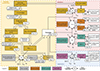 |
Fig. 1. Graphical representation of the entire process described in this paper. |
2. Performing a PCA
To build LC templates for Cepheids, we used the PCA approach. This method is particularly suited to such a study as the shape of the LC is mainly driven by the mass of the Cepheid (Balázs & Kovács 2025). The PCA allows us to extract the main shape of the curve and characterise it using a small number of components, with as many parameters. A mathematical description of the principle of PCA can be found for instance in Deeming (1964). In short (and in the context of the application to LCs), the PCA can be used to find a proper base of function in which a given training set can be decomposed. These functions are orthogonal to avoid redundant information and by ordering them by their order of magnitude in the training set, we can choose to reduce the dimension of the base of functions to keep the most relevant parts. In this work, we refer to the different base functions (or base vectors) as Ci, with i being an integer from 1 to the dimension of the PCA, which depends on the training sample. We set the C0 component to be the mean function of the training sample, which will always be weighted similarly. Each vector, f, can then be represented as a linear combination of the base vectors, (Ci)i ∈ {0, …, k}, as follows
 (1)
(1)
In the following, we explain how we determined the set of vectors that best describes the range of LCs.
In this analysis, we base our template generation on various datasets. We defined three particular samples, named ‘gold’ for the training sample of the PCA, ‘silver’ for the sample used to derive the relations between the period and the shape of the LC, and ‘bronze’ for the main validation sample. Each sample is composed of a specific selection of Cepheids depending on the available observational data. The use of these samples in our PCA implementation is visually described using colour-coded boxes in Fig. 1.
2.1. Training datasets
We trained our PCA in all filters of interest using previous pulsation parametrisation of Cepheids. We made use of the Spectro-Photo-Interferometry for Pulsating Stars (SPIPS) results of a set of 75 Cepheids. The details of the SPIPS analysis method can be found in Mérand et al. (2015). The general idea was to combine observations from different techniques: spectroscopy for radial velocity (RV) and effective temperature, interferometry for angular diameter, and photometry in different passbands. We fit them using a phase dependent pulsation model. The parametrisation is composed of an RV curve, an effective temperature curve and a set of stellar parameters. Atmospheric models (from Castelli et al. 2003) were used to compute the synthetic LC in the different filters. Any filter can be used, providing its wavelength passband is known. This allows us to obtain photometric LC predictions for the modelled stars in every filter, including filters for which no observations is available. This is a strong advantage of the SPIPS tool, as Cepheids are observed in various photometric systems, but the heterogeneity of the photometry can be a problem when calibrating from one system to another. Instead, here, we are considering these various observations simultaneously, allowing us to cross-check their consistency. The use of the SPIPS parametrisation is particularly powerful as the predicted LC depends on interpolations using Fourier series of the radial velocity and effective temperature curves, which provides fits to all the observables. The predicted LCs show less unphysical behaviour, even in bands where the phase coverage is sparse. In this paper, we sometimes refer to these results as pulsation models, but it has to be noted that they are distinct from hydrodynamical pulsation models. This is only a mathematical parametrisation, which allows us to reproduce the different observables in the pulsation of a Cepheid.
To train the PCA, we accumulated the gold sample comprising of 63 Cepheids whose χ2 values for the fit are low and their observed curves are well-reproduced from the large sample presented in Trahin et al. (2021). This sample was supplemented by 12 other fits that were considered to be of sufficient quality. We were particularly careful to check the satisfactory reproduction of the LCs in the different passbands that does not introduce spurious features. The list of stars used for the training sample is given in Table E.1, with the references of the data used for the SPIPS parametrisation. An example of these additional fit results is given in Fig. B.1. We tried to find a balance between the periods of the stars in the gold sample; however, a reliable SPIPS fit relies on precise and well-sampled photometry and spectroscopy (at least) and preferably with interferometric measurements. For this reason, our sample includes a lot of nearby Cepheids, with quite short periods, which we chose to keep to avoid reducing the size of the training sample. The distribution in terms of the period of the training sample is shown in gold in Fig. 2. In Fig. 1, we synthesise the steps of the processing for the Cepheid LCs in the gold sample (gold boxes).
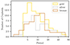 |
Fig. 2. Histogram of periods of Cepheids in the samples described in this paper. |
To gain efficiency in the analysis of extragalactic Cepheids and versatility for the LC fitting of Cepheids in general, we aimed to generate templates that combine information from all photometric observations at one time. This can be done by performing only one PCA on all filters at the same time, which is possible by generating photometry in any given list of filters for any star in the gold sample. In a technical aspect, we concatenated all LCs in the different filters in one single vector for the PCA (see Fig. 3). In the process, the mean temperature of the Cepheid is intrinsically incorporated when we perform the PCA, taking into account the differences in magnitude in the different bands. This method also allows us to drastically limit the number of parameters in the final templates. For this work, we arbitrarily chose a set of filters commonly used in ground-based observations for galactic Cepheids (BVRI Johnson, JHK) to validate our templates, but also HST and JWST filters to apply the templates to extragalactic Cepheids, which can be extended. We computed the synthetic LC for every star in our gold sample in the same selection of 43 filters. The list of the filters with the adopted mean wavelengths and labelled with the name that should be used when applying the templates is provided in the attached file. We include the V filter in the Walraven system, which is not in the same magnitude scale as the other filters. However, thanks to the numerical approach of the PCA, we have been able to use the direct magnitudes observed in this system, without recalibration. The change of scale will be encoded in the difference in magnitudes between this filter and the other filters, especially other filters in the V band.
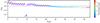 |
Fig. 3. Concatenated LC of RS Pup as one vector of the training sample for the PCA. Each sawtooth corresponds to one filter, colour-coded by its central wavelength. The LC around −6 in magnitude corresponds to the V Walraven system, which explains why it scales so differently from the other bands. |
All synthetic LCs were corrected for their apparent distance moduli, using distances from Gaia DR3 (Gaia Collaboration 2021; Lindegren et al. 2021) and from the reddening. The SPIPS parametrisation corrects for the reddening taking into account the temperature of the star at each pulsation phase. Generally, the correction is applied by integrating the Aλ parameter over the photometric passband ponderated by a standard Vega stellar spectrum. Because Cepheids are much cooler than 10 000 K, this can introduce an inaccurate correction from the interstellar dust, particularly in the broad filters. In practice, as observed by Trahin et al. (2021), the SPIPS approach of the reddening correction will convert into larger values for the colour excess E(B − V) than reported in the literature. For our templates, we simplified the SPIPS treatment by considering a constant temperature of 5500 K for all Cepheids during their whole pulsation phase. This is an approximation, but the variation induced in the reddening correction is very small compared to the variation with the classical approach of considering that all Cepheids have a constant temperature of 10 000 K. For this reason, all colour excesses that will be presented here are not in the same scale as the usual values for E(B − V) in the literature (for instance those collected by Breuval et al. 2021). We can estimate, however, how they relate to each other to compare and apply the literature estimations, from the following formula and using the Fitzpatrick (1999) reddening law,
 (2)
(2)
A photometric correction for circumstellar environments (CSEs) is also possible in SPIPS, using a power law parametrisation. The photometric contribution from such an envelope has been preserved in the derived LCs. Indeed, we used the LCs that offer a good match to the observations, as extragalactic Cepheids can also have CSEs (Gallenne et al. 2017). Finally, the vectors used in the PCA are normalised individually for each star, so the concatenated LC has a zero-mean value. This results in one unique additional parameter to reproducing the observations from such decomposition. We plotted the vector that corresponds to the long-period Cepheid RS Pup in Fig. 3 as an example. In this figure, the magnitude level of each sawtooth is important and is directly related to the temperature of the Cepheid only and specific to an unreddened star. Only the concatenated curve has been normalised, which explains why when looking at specific filters, the mean value will not be zero.
Our selection of stars is only composed of Galactic Cepheids, with solar-like metallicities. As it is possible that the metallicity of the star changes the shape of its LC, identified through the distribution of Fourier interpolation coefficient by, for instance, Hocdé et al. (2023), the present templates are only suitable for solar-like metallicities. An extension for metal-poor stars is discussed in Sect. 6.
2.2. Analysis
The PCA was performed using the implementation in the scikit-learn Python library (Pedregosa et al. 2011). The synthetic LCs are sampled at 0.001 in phase for all filters, while 75 components are kept in this computation to account for the variations in the 75 stars.
To reduce the number of dimensions, we extracted the components that account for the major differences in terms of shape. We assumed that the presence of peculiar small bumps that appear randomly in the LCs of certain stars will be represented in minor components; this is not crucial in our templates as these features are not important for the determination of mean magnitudes.
We retained the first four components, which explain 96.5% of the variance in the training sample, as shown in Fig. 4. This is similar to the findings of Javanmardi et al. (2021), where four components explained 97.1% of the variance, with a smaller sample and long-period Cepheids only. The large significance of a small number of components is expected from the SPIPS parametrisation, which is mainly encoded in the variations of the star’s radius and temperature. Beyond the fifth component, variations in the LC shape become particularly small, while encoding smaller features such as bumps. Also, the coefficients associated to the fifth component does not seem related to the period. We have aimed to retain only the variance related to the period to obtain meaningful templates. Including more components would be useless, as the interpolation of a coefficient to the period compensates for the added information. When adding the fourth component, the induced variation in mean magnitudes is smaller than 0.1 dex for every filter used, which explains why we stopped at four components.
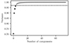 |
Fig. 4. Explained variance compared to the number of components considered. The dashed line corresponds to 97% of the variance of the training sample reproduced, acting as our threshold for the templates. |
Following the vectors in the training sample, the components are a concatenation of the LCs in the different filters. To obtain the components in a specific filter, we only need to take a truncation that corresponds to the given filter. This was done in Fig. C.1, where we plot the mean curves and the four first components for the V and K filters.
2.3. Coefficient distribution
It is interesting to find links between the empirical coefficients of the PCA and physical properties using the stellar parameters derived by SPIPS. We note that the effective temperature of the star constrains the coefficient of the first PCA component, as shown in Fig. 5. The temperature is the most important parameter as it drives the difference in magnitude among the different filters, which means that the first component generally defines the mean magnitude for each filter. Its close correlation with the luminosity and, therefore, the period of the star is crucial to building templates characterised by the period only.
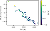 |
Fig. 5. Distribution of the coefficient associated to the first component with respect to the effective temperature of the star, derived by SPIPS. The metallicity from Breuval et al. (2021) is represented in colours. |
3. Generation of templates
3.1. Relation between the period and the coefficients
To define our set of templates, we need to predict the coefficients associated with the PCA from the period only, as it is the other parameter required to produce the PL relation. Deriving linear relations does not seem appropriate for each of the four components. However, for each period, we can estimate the probable values for the coefficients of the PCA from the mean value of the distribution of the coefficients of stars with similar periods. This leads us to define relations by using a moving average with a Gaussian weight. The standard deviation of the Gaussian weight was tuned manually and set to 0.07 in logarithmic scale to account for the variations of the coefficients without introducing unrealistic oscillations in terms of periods. From this method, we also estimated a confidence interval for the final templates from the dispersion of the coefficients for a certain period range. The distribution and the corresponding relations are shown for the four main components in Fig. 6. This averaging method will lead to smooth the variety of LCs in a same period range, which means averaging over the width of the instability strip and, in particular, they will average over the range of amplitudes of a given period bins as the amplitude of the LC of a Cepheid is not purely correlated to the pulsation period. As it could then be biased by the distribution of the instability strip, we plot in Fig. 7 the positions in the Hertzsprung–Russel diagram for the 75 stars in the gold sample.
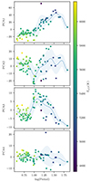 |
Fig. 6. Distribution of the coefficients associated to the four main components of the PCA as a function of the period, with the relation from a moving average with a Gaussian weight. The shaded area is the confidence interval derived from the standard deviation of the coefficients. |
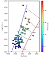 |
Fig. 7. Distribution in the instability strip of the 75 stars in the gold sample. The edges of the instability strip and the predicted periods are plotted according to Anderson (2016), for the first crossing, with a rotation of ωini = 0.5 and a solar metallicity of Z = 0.014 for comparison. |
Our relations are currently defined over a period ranging from 3.7 to 68.6 days, limited by the stars in our training sample. In nearby galaxies, it is common however to observe Cepheids with longer periods. Without any longer period Cepheid to increase this range, we used an extrapolation for relations between the period and the coefficients, assuming that the trend followed by these relations is also followed for longer periods and that the small number of long-period Cepheids considered here are representative.
3.2. Addition of a supplementary dataset
We were motivated by the lack of SPIPS results for very-long-period Cepheids to expand our dataset by including stars that are not in the gold sample, but for which good photometry was available from the literature. For this additional dataset, the silver sample, we made use of good photometric observations of Cepheids for which the SPIPS tool was not able to converge (due to a lack of spectroscopic data, e.g. either temperature or RV). With no model for the radius and the temperature of the star, we were not able to build the LC in any filter that we liked. Hence, we could not use this dataset as a proper training sample for the PCA, but we can use the fully phase-covered photometric data, as shown in the silver boxes in Fig. 1.
The silver sample is composed of a selection of 48 stars from the phase coverage of their LCs in various different filters, including IR filters. The main properties and references of datasets for the stars in this sample are tabulated in Table E.1. Photometric observations of stars in the silver sample werefitted using the principal components, Ci, obtained from the gold sample, leaving the associated coefficients, Ki, free. The colour excess is fixed to literature determinations, rescaled with ourfactor of 1.16 as defined in Eq. (2), to break the degeneracy with the temperature and, hence, the coefficient K1. In SPIPS, data are phased taking the maximum bolometric luminosity as a reference. This quantity is generally unknown for the stars in the silver sample as it relies on the global pulsation model, which we do not have. We thus included an offset parameter to take into account the difference in the reference date in fraction of period in the processing of the photometry of the stars in the silver sample. One unique parameter for all filters is used to scale the luminosity of the star, which we call the reference magnitude, mref. It acts as a global additive offset in magnitude and takes into account the normalisation of the vectors in the PCA and the distance modulus of the star.
The detailed parametrisation is the application of the PCA, as described by Eq. (1), where the f function is the magnitude, offseted by the reference magnitude, mref, is given in Eq. (3), with C0λ(ϕ) being the mean of the PCA and Ciλ(ϕ) the i-th components of the PCA in the filter at wavelength λ, coming from the PCA on the gold sample described previously. The components are associated with the coefficients Ki (independent of the filter). Here, Aλ is the correction from the interstellar extinction given the value of E(B − V) in the filter λ and dϕ is the phase offset to correct the date for the zero-phase. The mλ curve is only a truncated part of the whole vector containing all the filters,
 (3)
(3)
From this parametrisation, we set mref, the four Ki, and dϕ as free parameters, fitted to the data in all photometric bands simultaneously. We give an example of such a fit for the Cepheid SW Vel in Fig. 8. Each and every fit has been visually checked in order to keep the ones for which the LCs are well reproduced. The rejected ones were moved to the bronze sample (see Sect. 4). This sample allows us to increase the statistics to compute relations between the period and the coefficients associated to the PCA (hereafter, the P − Ki relations). We used the same moving average method as previously described, taking into account both gold and silver stars. We show them in Fig. 9.
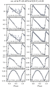 |
Fig. 8. Fit of SW Vel in the silver sample. The period and the E(B − V) are fixed. The predicted curves for several filters are shown in grey lines, the observations in silver-coloured points. |
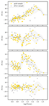 |
Fig. 9. Distribution of the Ki for the gold and silver samples. The moving average with a Gaussian weight and the confidence interval from the total distribution (gold and silver samples) are also plotted similarly as in Fig. 6. |
3.3. Templates and Hertzsprung progression
The derived P − Ki relations, together with the principal components Ci, allow us to predict the shape of the LC for a Cepheid of any period in any filter. An example of such a template is plotted in Fig. 10. This template is provided for the common V Johnson filter for a 20-day-period Cepheid, and J, H, and K CTIO filters are shown in Fig. D.1. The confidence interval shows the possible range for the particular features that we could observe for a Cepheid of this period. It does not represent a general offset of the curve.
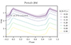 |
Fig. 10. Example of a template for a Cepheid of a period of 20 days. The different lines correspond to different values of E(B − V). The shaded area is the confidence interval and is given only for no interstellar reddening for readability. For other filters, see Fig. D.1. |
These templates naturally allow us to study how the LC shape evolves with the Cepheid’s period in any filter. We will focus on the common V Johnson filter, since the shape of the LC changes with the wavelength of the filter, as reported by Bhardwaj et al. (2015) in the context of the Hertzsprung progression. We plot different templates for periods between 6 and 40 days in Fig. 11 to show the evolution in the skewness of the LC. Around 10 days, we show particular change in the observed LC shape and the secondary bump of the Hertzsprung progression. This bump was first highlighted by Hertzsprung (1926) in the LCs of Cepheids between 6 and 14 days. In Fig. 11, even if this feature is smoothed during the template generation, we can still identify it (highlighted by the red arrows for LCs for 6 and 13 days).
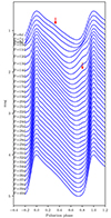 |
Fig. 11. Evolution of the shape of the LC with the period in the Johnson V band for periods from 6 to 40 days as predicted by our templates. The red arrow shows the secondary bump from the Hertzsprung progression. |
The Hertzsprung progression can also be characterised by the centre period of the progression, around which bump Cepheids are found. Marconi et al. (2024) showed, using theoretical models compared to observations in the Gaia database, that the centre of the Hertzsprung progression corresponds to a local minimum in the variation of the peak-to-peak amplitude with respect to the pulsation period, in the Gaia G band. The evolution of the amplitude of the LCs in our templates is shown in Fig. 12. The central period is located at 8.67 days, knowing that the mean metallicity of our sample is around 0.07 (individual metallicities are from the compilation by Breuval et al. 2021, and references therein). This is compatible with the results in Marconi et al. (2024), who reported the central period in this band is between 7.5 and 9.5 days, with longer period associated to lower metallicities, with the trend being confirmed by the theoretical models.
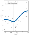 |
Fig. 12. Amplitude of the template LC in the Gaia G band and its evolution with the period from 6 to 16 days. The amplitude from the Gaia LC for the stars in the gold sample are also plotted for comparison with real data. |
4. Validation of the template LCs
In this section, we validate the derived templates with respect to how well they reproduce the multi-band LCs and their shapes. We describe its performance both internally and externally.
4.1. Search for systematic errors
As our templates are suited for the determinations of mean magnitudes, we need to estimate the error in this parameter. This can be done by comparing the predicted mean magnitudes from templates to the one retrieved by a fit of an LC using standard methods, such as the Fourier series. In both cases, the mean magnitudes were computed by converting into magnitude the average flux in the different filters.
We performed this analysis in two steps, using similar methods. First, we propose an internal validation using the training sample (gold sample) and an external validation using an independent validation sample (bronze sample). They are represented in the top part of the left panel of Fig. 1
For the internal validation, the 75 stars of the gold sample were fitted with the templates and the P − Ki relations without introducing the prior knowledge on the coefficients Ki. Only two parameters were fitted in this process; the reference magnitude, mref, and the colour excess, E(B − V). We show, as an example, the LC fitting for the Cepheid η Aql in Fig. 13. Interestingly, for this star, the bump present in the V band is not reproduced by the template, which smooths the curve at these phases. This feature is supposed to be too small to have an impact on the mean observed magnitude. We also plot the LC in the V band from the templates described in Yoachim et al. (2009). For this template, the secondary bump is also not fitted and the amplitude seems to be underestimated.
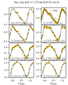 |
Fig. 13. Fitting procedure of η Aql in the gold sample, as a validation of the templates. Only two parameters are fitted to all the observations, mref and E(B − V). |
In Table 1, we compare the mean magnitudes from the fitted template to the mean magnitudes in the SPIPS results and from a Fourier interpolation of the LC when the phase-coverage is sufficient. For the reference comparison, we used determinations from several works (Monson & Pierce 2011; Gaia Collaboration 2018; Breuval et al. 2021; Gaia Collaboration 2023). The comparison with the SPIPS results provides us proof of self-consistence of the process and is used to validate the approach of P − Ki relations. The small offsets and dispersion found here indicate that while our templates smooth the LCs by omitting high-frequency terms, they remain effective in obtaining accurate mean magnitudes across all filters.
Distribution (average and standard deviation) of errors between mean magnitudes from a template fitting process and reference values from the literature.
For most photometric bands, we can see from the mean error that the mean magnitude is well retrieved, except for Gaia G and BP bands, especially for the DR3. Between the two latest data releases, the photometric passbands of Gaia have been recalibrated and the shape of the distribution in wavelengths have changed quite drastically. This explains why so much difference is obtained in the modelled magnitudes from atmospheric models. The problem for the newly calibrated passbands in the DR3 may lie in the difficulty for atmospheric models used in SPIPS to get a good photometry in the bluer bands, as stated by Casagrande & VandenBerg (2014). Although this problem is concerning in the context of using Gaia data more extensively, it does not impact the prediction in the other bands. We however note that the calibration of Gaia passbands from the DR2 seems to provide good predictions for the LC, even when compared to Gaia DR3 data. A quite large offset is also found for mean magnitudes in JHK filters in the 2MASS system (0.07 mag in H). This is surprising as the reference mean magnitudes that are quoted are computed from the same data sample as used in the template fitting, which were in the CTIO system, transformed into the 2MASS system, using transformation relations from Monson & Pierce (2011). A similar offset is found by comparing the LCs in JHK in the 2MASS system from our templates directly with the transformation using the same relations of the predicted LCs in JHK in the CTIO system. Given this comparison, and the fact that the photometry from the 2MASS survey seems to be well-fitted (even though one data point is clearly not sufficient to validate the fit), we conclude that this offset comes from the transformation relations between the CTIO and 2MASS systems. A comparison with the literature in HST filters will be discussed in details in Sect. 4.2.
The bronze sample is composed of 34 stars with available photometry both in the visible and the NIR, but not used for the template generation (neither in the gold nor in the silver sample). In particular, we selected stars that were already studied for the calibration of the Period-Wesenheit relations in HST filters (Riess et al. 2021). Photometric data for these stars come from various references, listed in Table E.1. We fit a template at the pulsation period of the star taken from the International Variable Star Index (VSX) database1 or, alternatively, from Berdnikov (2008). We left the reference magnitude, the colour excess, and an offset in phase as free parameters. Due to the heterogeneity in observation epochs (spanning many periods), the phasing of the data can be highly sensitive to the given period. Before the template fitting, we found a variation in the period (as a fraction of the initial period), by minimizing the dispersion in the phase-folded LCs to obtain cleaner phase-folded LCs in all filters. This was done independently of any predicted LC, avoiding a degeneracy with the template fit. The resulting period is used only for phasing and not to define the template as variations are supposed to be minimal. While this step has little impact on the retrieved mean magnitudes, it helps visualise the agreement between the template and observations. We do not claim to have a high level of precision in terms of the derived period, as we only aim to phase our data. In particular, period changes were not accounted for to maintain a low number of degrees of freedom. Finally, for extragalactic Cepheids, this step becomes less critical due to shorter time spans between epochs and noisier photometry, except when combining HST and JWST data. An example of fit of the LC for the Cepheid YZ Car using our templates is given in Fig. 14. We also show in the V and I bands (as done in Fig. 13), the LCs from the templates described in Yoachim et al. (2009). Both templates are especially similar in shape for this star.
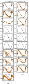 |
Fig. 14. Example of template fitting (grey lines) on YZ Car in the bronze sample. Observations are shown in bronze-coloured points and crosses. Crosses show data that are excluded from the fitting procedure. |
In the fitting procedure, we ignored a few specific filters that are not reproduced well by the template, but also generally in the SPIPS analysis. This accounts for blue filters (Johnson U for instance), but also other filters that are usually not included in the SPIPS analysis (R, Ic Johnson). For more information regarding the filters discarded in the SPIPS analysis, we refer to the SPIPS papers (e.g. Mérand et al. 2015; Breitfelder et al. 2016; Trahin et al. 2021; Bras et al. 2024).
Table 2 gives the statistical difference between the mean magnitudes predicted by the templates and a mean magnitude from a reference paper (Monson & Pierce 2011; Breuval et al. 2021; Gaia Collaboration 2023). These results were used to define the best choice for the width of the box in the moving average procedure to determine the P − Ki relations.
4.2. Validation with the SH0ES sample of Galactic Cepheids
In this section, we focus on stars in the sample described in Riess et al. (2021). Among these stars, 28 are in our gold sample, 12 in our silver sample, and 23 in our bronze sample; for the remaining 10 stars, we were not able to find any NIR photometry (except for 2MASS single measurements) to have confidence in the fit and add them to the bronze sample. We included these stars in the ‘bronze +’ sample to allow for some comparison. In Fig. 1, this step corresponds to the green boxes in the bottom of the validation panel.
We fit the photometry of all stars with the described templates, with the same free parameters: a reference magnitude, the colour excess, and a phase offset, except for the gold sample for which the data are already phased taking the maximum in bolometric luminosity as a reference. The LCs in the HST bands are predicted from the data in the other bands and are not based on any actual measurement. We also express the mean magnitudes in the Wesenheit index, defined as WH = F160W − 0.386(F555W − F814W) (Riess et al. 2021). In our case, we can produce an LC in the Wesenheit index and compute its mean magnitude or we can (as done in the literature) express the mean magnitudes in WH from the mean magnitudes in the F160W, F555W, and F814W filters. As the comparison from the second option is intrinsically given through the comparison of mean magnitudes in the other filters, we here compare the Wesenheit magnitude from Riess et al. (2021) with the mean magnitude from our templates constructed in the Wesenheit index. This enables us to validate more deeply the relation between the shape of the different LCs.
We compare the mean magnitudes in the HST bands with the mean magnitudes in Table 1 of Riess et al. (2021) in Fig. 15 and Table 3. We removed the correction from the count-rate non-linearity of the IR detector in Table 1 in Wesenheit magnitudes in Riess et al. (2021), to compare the actual measurements to the results of our templates. The standard deviation in the difference in mean magnitudes retrieved gives a hint on the precision we can achieve from such a method, which still depends on the number of filters for which photometry is available and is of order of the dispersion observed by Riess et al. (2021) when comparing their photometry to literature photometry (see their Fig. 1). It is not comparable to the precision from direct measurements of the LCs in those filters, but should be representative of the errors using the template fitting approach. However, without individual measurements in the filters considered here, it is difficult to decide whether the offset and the dispersion we observe come from bad fits of the LCs or from systematics in our method. However, this offset does not have clear consequences for the distance ladder as we still need to compare Cepheids in anchor galaxies and in distant galaxies with the same tool and this offset would presumably be the same in both cases.
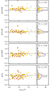 |
Fig. 15. Difference in mean magnitudes retrieved from the template with the mean magnitude in Riess et al. (2021) (mThis work − mRiess2021). The colours correspond to the gold, silver, and bronze samples accordingly. The right panel shows the distribution. The black unfilled step is for the whole sample. Bronze crosses are for stars without NIR photometry. They are added to the bronze sample to give the unfilled bronze step distribution in the right panel. |
Our approach also enables us to determine the colour excess given the magnitudes in the different filters. We provide in Fig. 16 a comparison with previous determinations in the literature, from Breuval et al. (2021), multiplied by our 1.16 factor (see Eq. 2).
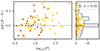 |
Fig. 16. Difference in E(B − V) retrieved from the template fitting with determinations from Breuval et al. (2021). The legend is the same as for Fig. 15. |
4.3. Validation of the LC shape
Besides the mean magnitudes, this section aims to investigate how well the LC shape is reproduced. We made use of our previous template fitting of our bronze sample to compare zero-mean LCs in each filter, as synthetised in the middle part of the validation panel in Fig. 1.
The comparison of the shape can be made by comparing the produced template with a parametrisation from a Fourier decomposition, as commonly done in the literature. A possible reference for such a decomposition could be the Gaia parameters, but as the Gaia bands are quite badly reproduced with by templates, it is not well suited for that purpose. Bhardwaj et al. (2015) provided the first Fourier parameters for a large number of stars in the V band and for a smaller number of stars in JHK bands; thus, it is fully adapted for the purposes of our investigation as well. Both computed curves were phased to minimise the total difference between them. We differentiated only among the differences in the shape of the curve, thus, we did not consider a possible offset in magnitude and we simply retrieved the intensity-averaged magnitude for the Fourier interpolation and the template independently. The observations were plotted to visually check whether the variations in shape come from real observations or from an oscillation in the Fourier interpolation. An example is given in Fig. 17. The template curve shown here is only dependent on the period of the star (due to the normalisation in terms of magnitude) and not on any observation or fitting process.
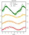 |
Fig. 17. Shape validation of AA Gem (bronze sample). We compare the template, associated to the period of the star, and the Fourier interpolation of observations from Bhardwaj et al. (2015). |
We plot in Fig. 18 the normalised difference between the template and the Fourier interpolation for the V-band LCs of all stars in our bronze sample, except AP Pup (as it has no Fourier decomposition in Bhardwaj et al. 2015). The curves are shown colour-coded with the pulsation period of the star, but there do not seem to be any clear tendencies that ought to be highlighted. The standard deviation of the distribution (≤1) could suggest an overestimation of the confidence interval for the template; however, this may also account for the difference in the mean magnitude, which is not considered here.
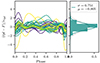 |
Fig. 18. Normalised residuals between the templates and a Fourier interpolation in the V band of stars in the bronze sample and its distribution (right panel). The Gaussian distribution is given for comparison in dashed black line. |
5. Fitting the templates to extragalactic Cepheids
As a proof of concept, here we present an application of our templates to extragalactic Cepheids, observed with the HST in the context of the SH0ES project (see the bottom of the left panel in Fig. 1, shown as purple boxes). We made use of the epoch photometry in four filters (F350LP, F555W, F814W, and F160W) derived by Javanmardi et al. (2021) from HST observations of the SNIa host galaxy NGC5584. However, it is interesting to note that this galaxy has been quite intensively observed and the number of data points for the Cepheids in this galaxy is not fully representative of the observations of SNIa host galaxies in general. Still, testing the template fitting on this galaxy is valuable in terms of demonstrating the potential of our method.
Our templates have allowed us to simultaneously use information from all filters to derive consistent parameters. However, the determination of the period is still a delicate matter. Using the templates in V and I bands of Yoachim et al. (2009), Hoffmann et al. (2016) tested several periods that were equally spaced in a logarithmic scale, involving a visual inspection. As this process can become computationally expensive, we suggest narrowing the probable period range using standard methods such as the Lomb-Scargle periodogram or the string-length method (see Giertych et al. 2024). For this example, we used a string-length method on both the F350LP and F555W filters, summing the string-length functions to determine a plausible period. We then explored ten starting periods, logarithmically spaced around this plausible period, with a range of ∼1 day around 20 days for the period and ∼20 days around 100 days for the period. For each trial period, we fit all the photometry with our templates and four free parameters:
-
the period (varying within the limit of the other trial periods);
-
a phase offset to align the reference in time;
-
the reference magnitude that offsets all LCs homothetically;
-
the colour excess E(B − V).
The fit was performed in two steps. First, we found the phasing parameters (period and phase offset) from a standard χ2 minimisation in the four filters simultaneously and selected the trial period with the lowest χ2. Because F160W has fewer observations, it has little impact on the phasing, which is mostly determined by LCs in the visible. However, these observations are critical for constraining the colour excess; hence, in the second step, we refined the reference magnitude and E(B − V), weighting the data by the number of observations per filter, using fixed phasing parameters. Uncertainties were derived by fitting random realisations of observations within their error bars. A result of such a fit (Fig. 19 in this work) is given for one of the representative Cepheids given in Hoffmann et al. (2016, specifically, Fig. 4) and Javanmardi et al. (2021, specifically, Fig. 7).
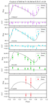 |
Fig. 19. Example of the Cepheid 473829 in NGC 5584. For each filter the observations, the fitted template, and the residuals are plotted. Data come from the work of Javanmardi et al. (2021). |
We compare our parameters for the presented Cepheid with previous estimations in Table 4. From a visual inspection of the curves, we would like to lower the magnitude in the F160W filter and increase the magnitude in the F814W filter. This is not possible in our multi-band approach as differences of mean magnitudes are fully determined by the period through the template and the colour excess. A better constraint on IR filters would be very valuable and we are making progress in adding JWST data to improve the template fitting process. Adding in these data will certainly improve our results even in the HST bands, as we will determine the colour excess more accurately. This means that we have access to dereddened magnitudes to obtain the period-luminosity relation in the visible range, without the scatter introduced by reddening effects. From the visualisation of the fit, it seems that we are underestimating the magnitude in F814W, probably because of an error in the determination of the colour excess. In the F160W filter, we obtained a mean magnitude that is lower than both previous determinations. However, increasing this magnitude does not seem to fit well with the data showed in Fig. 19.
Properties of the Cepheid 473829 in NGC5584.
6. Discussion
In this section, we point out some improvements to the present work or future paths that might be followed to extract the complete potential of these templates.
First of all, we emphasise that our generated templates are mainly aimed to the estimation of mean magnitudes in different filters. They are not properly suited for an interpolation of a well-observed Cepheid with good phase coverage, unless we relax the constraint on the coefficients associated to the PCA. In particular, they will not reproduce the amplitude of any Cepheid exactly or specific features like the bump of the Hertzsprung progression, because the goal in this work has been to link the general shape of the LC to the pulsation period only.
It is important to treat the reddening issue meticulously, as it has an important role in the mean magnitudes in the different filters. For the generation of our templates, we used appropriate corrections from the reddening due to interstellar dust, taking into account the fact that Cepheids have temperatures around 5500K, which has a significant impact on the photometry in broad filters such as F350LP. The present work enables us to study the suitable RV parameter for reddening laws in various other galaxies and the reddening law itself (see also Mörtsell et al. 2022, for a discussion on the characterisation of reddening laws between anchor and SNIa host galaxies), as we have been able to study dereddened PL relations in the different filters. These questions are not raised by the standard approach by the SH0ES team as they used the Wesenheit index, rather than via the RW parameter, in defining the Wesenheit magnitudes.
On the other hand, metallicity has a limited impact on the distance scale as it is quite similar in SNIa host galaxies and in the MW (Riess et al. 2022), which explains why we considered the galactic metallicity in this work. However, it seems to have an impact on the shape of Cepheids LCs (Hocdé et al. 2023), and was proven to be particularly striking for short-period Cepheids (below 6 days). For longer periods, it is possible that the variation in the shape would occur at higher frequencies. This raises the question of whether this effect would impact the template fitting to metal-poor Cepheids in the Magellanic Clouds, for instance. It would be interesting to quantify this effect based on our previous analysis. Using our principal components, we could study the LCs of low-metallicity Cepheids and analyse the coefficient distribution. This could reveal analogous Cepheids (in terms of shape and luminosities) when going to lower metallicity, but a longer period.
Moreover, in this approach, we include in our templates the potential contribution from CSE, by making the hypothesis that their impact is homogeneous in galactic and extragalactic Cepheids or its presence will add dispersion to the P − Ki relations. It is then important to understand the CSE properties across the instability strip to reduce the uncertainty of our templates and (if it does indeed exist) the link between the CSE and the metallicity. So far, no particular correlation with the location on the instability strip could be identified by Gallenne et al. (2021). They also highlighted that the impact of the CSE mainly results in a variation in the ratio of magnitude between the different filters, which will likely be absorbed in the fitted parameters mref and the colour excess, E(B − V).
Finally, we introduced the algebraic parameter mref to move all LCs in all filters homothetically, which depends on the filters used at the beginning of our analysis and does not have a proper physical meaning, but we note that it is similar to a distance modulus. The result is that for more distant Cepheids, the template fitting procedure will give higher values for mref, as all magnitudes in all filters will be higher. We could think of another parametrisation of the PCA where this parameter would be directly linked to the distance of the Cepheid. The only free parameters will then be reduced to the distance, the reddening, the period, and a time reference. By doing so, the calibration of the PL relation would be incorporated into the P − Ki relations directly and will no longer be needed, as the fit with such derived templates would also estimate the distance. This could help in setting better constraints on the uncertainties when fitting extragalactic Cepheids in future studies.
7. Conclusion
We present a new approach to constructing LC templates for Cepheids, which intrinsically includes the information of the temperature of the star and a proper correction for the reddening from interstellar dust, with the limitation that they are not able to reproduce the variety of Cepheid LCs in the same period bin. This approach allows us to apply these templates to a broad variety of science cases, thanks to their versatility in terms of the photometric filters used. They incorporated a physical understanding of the variation of the photosphere, through the use of SPIPS parametrisation for the training sample. In our study, we introduced different validation samples in order to test the possibilities of the use of such templates. We recommend the user to adapt the template fitting procedure to their scientific question. In particular, if the aim is to fit the shape of the LC with a good phase coverage for the data, but a large number of filters, it would be necessary to allow some variation in the shape of LCs by relaxing the constraints on the values of the coefficients associated to the PCA, to retrieve fine features. We have also demonstrated their application in the case of extragalactic Cepheids for the distance ladder.
These templates will be used for an independent analysis of HST images of the sample of SNIa host galaxies studied in Riess et al. (2022) to validate the second rung of the distance ladder performed by this team, together with new photometry of the stars in these galaxies. The result will be published in a forthcoming paper. The templates will also be pertinent to interpret JWST data. We are already able to produce LCs of Cepheids in JWST filters and including them for extragalactic Cepheids will be feasible without the need for any new analysis.
Data availability
The necessary data to reproduce the analysis is accessible on Zenodo (https://zenodo.org/records/15102197). The record contains the fits output files of the SPIPS analysis of the 75 stars of our gold sample and a fits file including all the information to generate LC templates (extinction coefficients for the selection of filters, principal components and P − Ki relations).
Operated at AAVSO, Cambridge, Massachusetts, USA.
Acknowledgments
This work has made use of data from the European Space Agency (ESA) mission Gaia (http://www.cosmos.esa.int/gaia), processed by the Gaia Data Processing and Analysis Consortium (DPAC, http://www.cosmos.esa.int/web/gaia/dpac/consortium). Funding for the DPAC has been provided by national institutions, in particular the institutions participating in the Gaia Multilateral Agreement. The research leading to these results has received funding from the European Research Council (ERC) under the European Union’s Horizon 2020 research and innovation program (projects CepBin, grant agreement 695099, and UniverScale, grant agreement 951549). This research has been supported by the Polish-French Marie Skłodowska-Curie and Pierre Curie Science Prize awarded by the Foundation for Polish Science. The authors acknowledge the support of the French Agence Nationale de la Recherche (ANR), under grant ANR-23-CE31-0009-01 (Unlock-pfactor). A. G. acknowledges the support of the Agencia Nacional de Investigación Científica y Desarrollo (ANID) through the FONDECYT Regular grant 1241073. We also acknowledge support from the Polish Ministry of Science and Higher Education grant DIR-WSIB.92.2.2024. This research has made use of Astropy (Available at http://www.astropy.org/), a community-developed core Python package for Astronomy (Astropy Collaboration 2013, 2018), the Numpy library (Harris et al. 2020), the Astroquery library (Ginsburg et al. 2019), the scikit-learn package (Pedregosa et al. 2011) and the Matplotlib graphics environment (Hunter 2007). We acknowledge with thanks the variable star observations from the AAVSO International Database contributed by observers worldwide and used in this research. We used the SIMBAD and VizieR databases and catalogue access tool at the CDS, Strasbourg (France), and NASA’s Astrophysics Data System Bibliographic Services. The original description of the VizieR service was published in Ochsenbein et al. (2000). This publication makes use of data products from the Two Micron All Sky Survey, which is a joint project of the University of Massachusetts and the Infrared Processing and Analysis Center/California Institute of Technology, funded by the National Aeronautics and Space Administration and the National Science Foundation.
References
- Anderson, R. I. 2016, MNRAS, 463, 1707 [NASA ADS] [CrossRef] [Google Scholar]
- Astropy Collaboration (Robitaille, T. P., et al.) 2013, A&A, 558, A33 [NASA ADS] [CrossRef] [EDP Sciences] [Google Scholar]
- Astropy Collaboration (Price-Whelan, A. M., et al.) 2018, AJ, 156, 123 [Google Scholar]
- Balázs, L. G., & Kovács, G. B. 2025, New Astron., 116, 102317P [Google Scholar]
- Barnes, T. G., Fernley, J. A., Frueh, M. L., et al. 1997, PASP, 109, 645 [NASA ADS] [CrossRef] [Google Scholar]
- Berdnikov, L. N. 2008, VizieR Online Data Catalog: II/285 [Google Scholar]
- Bhardwaj, A., Kanbur, S. M., Singh, H. P., Macri, L. M., & Ngeow, C.-C. 2015, MNRAS, 447, 3342 [CrossRef] [Google Scholar]
- Bras, G., Kervella, P., Trahin, B., et al. 2024, A&A, 684, A126 [NASA ADS] [CrossRef] [EDP Sciences] [Google Scholar]
- Breitfelder, J., Mérand, A., Kervella, P., et al. 2016, A&A, 587, A117 [CrossRef] [EDP Sciences] [Google Scholar]
- Breuval, L., Kervella, P., Wielgórski, P., et al. 2021, ApJ, 913, 38 [NASA ADS] [CrossRef] [Google Scholar]
- Casagrande, L., & VandenBerg, D. A. 2014, MNRAS, 444, 392 [Google Scholar]
- Castelli, F., & Kurucz, R. L. 2003, in Modelling of Stellar Atmospheres, eds. N. Piskunov, W. W. Weiss, & D. F. Gray, 210, A20 [Google Scholar]
- Chown, A. H., Scowcroft, V., & Wuyts, S. 2021, MNRAS, 500, 817 [Google Scholar]
- Coulson, I. M., & Caldwell, J. A. R. 1985, South African Astronomical Observatory Circular, 9, 5 [Google Scholar]
- Coulson, I. M., Caldwell, J. A. R., & Gieren, W. P. 1985, ApJS, 57, 595 [NASA ADS] [CrossRef] [Google Scholar]
- Cutri, R. M., Skrutskie, M. F., van Dyk, S., et al. 2003, 2MASS All Sky Catalog of Point Sources [Google Scholar]
- Deeming, T. J. 1964, MNRAS, 127, 493 [NASA ADS] [Google Scholar]
- Engle, S. G., Guinan, E. F., Harper, G. M., Neilson, H. R., & Remage Evans, N. 2014, ApJ, 794, 80 [NASA ADS] [CrossRef] [Google Scholar]
- ESA 1997, in The HIPPARCOS and TYCHO Catalogues. Astrometric and Photometric Star Catalogues Derived from the ESA HIPPARCOS Space Astrometry Mission, ESA Special Publication, 1200 [Google Scholar]
- Feast, M. W., Laney, C. D., Kinman, T. D., van Leeuwen, F., & Whitelock, P. A. 2008, MNRAS, 386, 2115 [NASA ADS] [CrossRef] [Google Scholar]
- Fitzpatrick, E. L. 1999, PASP, 111, 63 [Google Scholar]
- Freedman, W. L. 1988, ApJ, 326, 691 [Google Scholar]
- Freedman, W. L., & Madore, B. F. 2010, ApJ, 719, 335 [Google Scholar]
- Gaia Collaboration (Brown, A. G. A., et al.) 2018, A&A, 616, A1 [NASA ADS] [CrossRef] [EDP Sciences] [Google Scholar]
- Gaia Collaboration (Brown, A. G. A., et al.) 2021, A&A, 649, A1 [NASA ADS] [CrossRef] [EDP Sciences] [Google Scholar]
- Gaia Collaboration (Vallenari, A., et al.) 2023, A&A, 674, A1 [NASA ADS] [CrossRef] [EDP Sciences] [Google Scholar]
- Gallenne, A., Kervella, P., Mérand, A., et al. 2017, A&A, 608, A18 [NASA ADS] [CrossRef] [EDP Sciences] [Google Scholar]
- Gallenne, A., Mérand, A., Kervella, P., et al. 2021, A&A, 651, A113 [NASA ADS] [CrossRef] [EDP Sciences] [Google Scholar]
- Gieren, W. 1981, ApJS, 47, 315 [Google Scholar]
- Gieren, W. P. 1985, ApJ, 295, 507 [NASA ADS] [CrossRef] [Google Scholar]
- Giertych, N., Shaban, A., Haravu, P., & Williams, P., Jr. 2024, Reports on Progress in Physics, 87, 078401 [Google Scholar]
- Ginsburg, A., Sipőcz, B. M., Brasseur, C. E., et al. 2019, AJ, 157, 98 [Google Scholar]
- Harris, H. C. 1981, AJ, 86, 707 [Google Scholar]
- Harris, C. R., Millman, K. J., van der Walt, S. J., et al. 2020, Nature, 585, 357 [NASA ADS] [CrossRef] [Google Scholar]
- Hendry, M. A., Tanvir, N. R., & Kanbur, S. M. 1999, in Harmonizing Cosmic Distance Scales in a Post-HIPPARCOS Era, eds. D. Egret, & A. Heck, ASP Conf. Ser., 167, 192 [Google Scholar]
- Hertzsprung, E. 1926, Bull. Astron. Inst. Neth., 3, 115 [NASA ADS] [Google Scholar]
- Hocdé, V., Smolec, R., Moskalik, P., Ziółkowska, O., & Singh Rathour, R. 2023, A&A, 671, A157 [NASA ADS] [CrossRef] [EDP Sciences] [Google Scholar]
- Hoffmann, S. L., Macri, L. M., Riess, A. G., et al. 2016, ApJ, 830, 10 [Google Scholar]
- Hunter, J. D. 2007, Computing in Science and Engineering, 9, 90 [Google Scholar]
- Inno, L., Matsunaga, N., Romaniello, M., et al. 2015, A&A, 576, A30 [NASA ADS] [CrossRef] [EDP Sciences] [Google Scholar]
- Javanmardi, B., Mérand, A., Kervella, P., et al. 2021, ApJ, 911, 12 [Google Scholar]
- Kanbur, S. M., Iono, D., Tanvir, N. R., & Hendry, M. A. 2002, MNRAS, 329, 126 [Google Scholar]
- Kervella, P., Trahin, B., Bond, H. E., et al. 2017, A&A, 600, A127 [NASA ADS] [CrossRef] [EDP Sciences] [Google Scholar]
- Kiss, L. L. 1998, MNRAS, 297, 825 [NASA ADS] [CrossRef] [Google Scholar]
- Laney, C. D., & Stobie, R. S. 1992, A&AS, 93, 93 [NASA ADS] [Google Scholar]
- Leavitt, H. S., & Pickering, E. C. 1912, Harvard College Observatory Circular, 173, 1 [Google Scholar]
- Lindegren, L., Bastian, U., Biermann, M., et al. 2021, A&A, 649, A4 [EDP Sciences] [Google Scholar]
- Lloyd Evans, T. 1980, South African Astronomical Observatory Circular, 1, 163 [Google Scholar]
- Madore, B. F. 1975, ApJS, 29, 219 [Google Scholar]
- Madore, B. F., Freedman, W. L., & Owens, K. 2024, AJ, 167, 201 [Google Scholar]
- Marconi, M., De Somma, G., Molinaro, R., et al. 2024, MNRAS, 529, 4210 [NASA ADS] [CrossRef] [Google Scholar]
- Mérand, A., Kervella, P., Breitfelder, J., et al. 2015, A&A, 584, A80 [NASA ADS] [CrossRef] [EDP Sciences] [Google Scholar]
- Moffett, T. J., & Barnes, T. G., I 1984, ApJS, 55, 389 [NASA ADS] [CrossRef] [Google Scholar]
- Monson, A. J., & Pierce, M. J. 2011, ApJS, 193, 12 [Google Scholar]
- Monson, A. J., Freedman, W. L., Madore, B. F., et al. 2012, ApJ, 759, 146 [Google Scholar]
- Mörtsell, E., Goobar, A., Johansson, J., & Dhawan, S. 2022, ApJ, 933, 212 [CrossRef] [Google Scholar]
- Ngeow, C.-C., Kanbur, S. M., Nikolaev, S., Tanvir, N. R., & Hendry, M. A. 2003, ApJ, 586, 959 [NASA ADS] [CrossRef] [Google Scholar]
- Ochsenbein, F., Bauer, P., & Marcout, J. 2000, A&AS, 143, 23 [NASA ADS] [CrossRef] [EDP Sciences] [Google Scholar]
- Pedregosa, F., Varoquaux, G., Gramfort, A., et al. 2011, Journal of Machine Learning Research, 12, 2825 [Google Scholar]
- Pejcha, O., & Kochanek, C. S. 2012, ApJ, 748, 107 [Google Scholar]
- Pel, J. W. 1976, A&AS, 24, 413 [NASA ADS] [Google Scholar]
- Phillips, M. M. 1993, ApJ, 413, L105 [Google Scholar]
- Pietrzyński, G., Graczyk, D., Gallenne, A., et al. 2019, Nature, 567, 200 [Google Scholar]
- Reid, M. J., Pesce, D. W., & Riess, A. G. 2019, ApJ, 886, L27 [Google Scholar]
- Riess, A. G., Macri, L. M., Hoffmann, S. L., et al. 2016, ApJ, 826, 56 [Google Scholar]
- Riess, A. G., Casertano, S., Yuan, W., et al. 2021, ApJ, 908, L6 [NASA ADS] [CrossRef] [Google Scholar]
- Riess, A. G., Yuan, W., Macri, L. M., et al. 2022, ApJ, 934, L7 [NASA ADS] [CrossRef] [Google Scholar]
- Schechter, P. L., Avruch, I. M., Caldwell, J. A. R., & Keane, M. J. 1992, AJ, 104, 1930 [NASA ADS] [CrossRef] [Google Scholar]
- Stetson, P. B. 1996, PASP, 108, 851 [NASA ADS] [CrossRef] [Google Scholar]
- Szabados, L. 1977, Commmunications of the Konkoly Observatory Hungary, 70, 1 [Google Scholar]
- Szabados, L. 1980, Commmunications of the Konkoly Observatory Hungary, 76, 1 [Google Scholar]
- Szabados, L. 1981, Commmunications of the Konkoly Observatory Hungary, 77, 1 [Google Scholar]
- Tanvir, N. R., Hendry, M. A., Watkins, A., et al. 2005, MNRAS, 363, 749 [Google Scholar]
- Trahin, B., Breuval, L., Kervella, P., et al. 2021, A&A, 656, A102 [NASA ADS] [CrossRef] [EDP Sciences] [Google Scholar]
- Walraven, J. H., Tinbergen, J., & Walraven, T. 1964, Bull. Astron. Inst. Neth., 17, 520 [NASA ADS] [Google Scholar]
- Welch, D. L., Wieland, F., McAlary, C. W., et al. 1984, ApJS, 54, 547 [Google Scholar]
- Yoachim, P., McCommas, L. P., Dalcanton, J. J., & Williams, B. F. 2009, AJ, 137, 4697 [NASA ADS] [CrossRef] [Google Scholar]
Appendix A: Python programme for using complementary data to generate templates of LCs
We present here a python script easy to run to produce template LCs for a Cepheid given a set of parameters that may be changed. The fits file needed is joined to this paper on Zenodo.
import numpy as np
from astropy.io import fits
from scipy.interpolate import interp1d
import astropy.units as u

# Read supplementary data
hdu = fits.open('PCA_data.fits')

# Parameters
photometric_band = 'V_GCPD_Johnson'
R_v = 3.1
Period_in_days = 20
mag_ref = 10
EBV = 0.5

# Compute template LC and its error
mask = np.where(hdu[1].data['Filter']==photometric_band)
LC = hdu[1].data['C0'][mask]
error_LC = np.zeros(LC.shape)

for i in range (1,5):
        Ki = interp1d(hdu[2].data['log_P'], hdu[2].data['K'+str(i)])(np.log10(Period_in_days))
        e_Ki = interp1d(hdu[2].data['log_P'], hdu[2].data['e_K'+str(i)])(np.log10(Period_in_days))
        LC += Ki*hdu[1].data['C'+str(i)][mask]
        error_LC += (e_Ki*hdu[1].data['C'+str(i)][mask])**2
error_LC = np.sqrt(error_LC)
LC += mag_ref + EBV*hdu[0].header['A_LAMBDA_5500K '+photometric_band]
Appendix B: Example of a SPIS fit for Cepheids in the gold sample
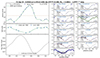 |
Fig. B.1. Pulsation parametrisation from the SPIPS fitting tool for YZ Sgr in the gold sample, but not included in Trahin et al. (2021). The χ2 for this fit is 1.92. |
Appendix C: PCA components for two filters
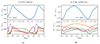 |
Fig. C.1. Mean LC (top) and the four first components (bottom) associated to the Johnson V (a) and CTIO K (b) filters. |
Appendix D: Example of templates for some standard filters
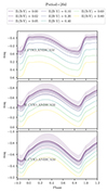 |
Fig. D.1. Example of a template for a Cepheid of a period of 20 days. The legend is similar as in Fig. 10 |
Appendix E: Properties of the stars used in this paper
Galactic Cepheids studied for the templates generation and validation.
All Tables
Distribution (average and standard deviation) of errors between mean magnitudes from a template fitting process and reference values from the literature.
All Figures
|
Fig. 1. Graphical representation of the entire process described in this paper. |
| In the text | |
|
Fig. 2. Histogram of periods of Cepheids in the samples described in this paper. |
| In the text | |
|
Fig. 3. Concatenated LC of RS Pup as one vector of the training sample for the PCA. Each sawtooth corresponds to one filter, colour-coded by its central wavelength. The LC around −6 in magnitude corresponds to the V Walraven system, which explains why it scales so differently from the other bands. |
| In the text | |
|
Fig. 4. Explained variance compared to the number of components considered. The dashed line corresponds to 97% of the variance of the training sample reproduced, acting as our threshold for the templates. |
| In the text | |
|
Fig. 5. Distribution of the coefficient associated to the first component with respect to the effective temperature of the star, derived by SPIPS. The metallicity from Breuval et al. (2021) is represented in colours. |
| In the text | |
|
Fig. 6. Distribution of the coefficients associated to the four main components of the PCA as a function of the period, with the relation from a moving average with a Gaussian weight. The shaded area is the confidence interval derived from the standard deviation of the coefficients. |
| In the text | |
|
Fig. 7. Distribution in the instability strip of the 75 stars in the gold sample. The edges of the instability strip and the predicted periods are plotted according to Anderson (2016), for the first crossing, with a rotation of ωini = 0.5 and a solar metallicity of Z = 0.014 for comparison. |
| In the text | |
|
Fig. 8. Fit of SW Vel in the silver sample. The period and the E(B − V) are fixed. The predicted curves for several filters are shown in grey lines, the observations in silver-coloured points. |
| In the text | |
|
Fig. 9. Distribution of the Ki for the gold and silver samples. The moving average with a Gaussian weight and the confidence interval from the total distribution (gold and silver samples) are also plotted similarly as in Fig. 6. |
| In the text | |
|
Fig. 10. Example of a template for a Cepheid of a period of 20 days. The different lines correspond to different values of E(B − V). The shaded area is the confidence interval and is given only for no interstellar reddening for readability. For other filters, see Fig. D.1. |
| In the text | |
|
Fig. 11. Evolution of the shape of the LC with the period in the Johnson V band for periods from 6 to 40 days as predicted by our templates. The red arrow shows the secondary bump from the Hertzsprung progression. |
| In the text | |
|
Fig. 12. Amplitude of the template LC in the Gaia G band and its evolution with the period from 6 to 16 days. The amplitude from the Gaia LC for the stars in the gold sample are also plotted for comparison with real data. |
| In the text | |
|
Fig. 13. Fitting procedure of η Aql in the gold sample, as a validation of the templates. Only two parameters are fitted to all the observations, mref and E(B − V). |
| In the text | |
|
Fig. 14. Example of template fitting (grey lines) on YZ Car in the bronze sample. Observations are shown in bronze-coloured points and crosses. Crosses show data that are excluded from the fitting procedure. |
| In the text | |
|
Fig. 15. Difference in mean magnitudes retrieved from the template with the mean magnitude in Riess et al. (2021) (mThis work − mRiess2021). The colours correspond to the gold, silver, and bronze samples accordingly. The right panel shows the distribution. The black unfilled step is for the whole sample. Bronze crosses are for stars without NIR photometry. They are added to the bronze sample to give the unfilled bronze step distribution in the right panel. |
| In the text | |
|
Fig. 16. Difference in E(B − V) retrieved from the template fitting with determinations from Breuval et al. (2021). The legend is the same as for Fig. 15. |
| In the text | |
|
Fig. 17. Shape validation of AA Gem (bronze sample). We compare the template, associated to the period of the star, and the Fourier interpolation of observations from Bhardwaj et al. (2015). |
| In the text | |
|
Fig. 18. Normalised residuals between the templates and a Fourier interpolation in the V band of stars in the bronze sample and its distribution (right panel). The Gaussian distribution is given for comparison in dashed black line. |
| In the text | |
|
Fig. 19. Example of the Cepheid 473829 in NGC 5584. For each filter the observations, the fitted template, and the residuals are plotted. Data come from the work of Javanmardi et al. (2021). |
| In the text | |
|
Fig. B.1. Pulsation parametrisation from the SPIPS fitting tool for YZ Sgr in the gold sample, but not included in Trahin et al. (2021). The χ2 for this fit is 1.92. |
| In the text | |
|
Fig. C.1. Mean LC (top) and the four first components (bottom) associated to the Johnson V (a) and CTIO K (b) filters. |
| In the text | |
|
Fig. D.1. Example of a template for a Cepheid of a period of 20 days. The legend is similar as in Fig. 10 |
| In the text | |
Current usage metrics show cumulative count of Article Views (full-text article views including HTML views, PDF and ePub downloads, according to the available data) and Abstracts Views on Vision4Press platform.
Data correspond to usage on the plateform after 2015. The current usage metrics is available 48-96 hours after online publication and is updated daily on week days.
Initial download of the metrics may take a while.