| Issue |
A&A
Volume 666, October 2022
|
|
|---|---|---|
| Article Number | A13 | |
| Number of page(s) | 10 | |
| Section | Cosmology (including clusters of galaxies) | |
| DOI | https://doi.org/10.1051/0004-6361/202243988 | |
| Published online | 29 September 2022 | |
The Hubble constant from two sibling Type Ia supernovae in the nearby galaxy NGC 4414: SN 1974G and SN 2021J
1
Instituto de Astrofísica de Andalucía (CSIC), Glorieta de la Astronomía s/n, 18008 Granada, Spain
e-mail: This email address is being protected from spambots. You need JavaScript enabled to view it.
2
DARK, Niels Bohr Institute, University of Copenhagen, Jagtvej 128, 2200 Copenhagen, Denmark
3
Department of Astronomy & Astrophysics, University of Chicago, 5640 South Ellis Avenue, Chicago, IL 60637, USA
Received:
10
May
2022
Accepted:
14
August
2022
Abstract
Having two “sibling” Type Ia supernovae (SNe Ia) in the same galaxy offers additional advantages in reducing a variety of systematic errors involved in estimating the Hubble constant, H0. NGC 4414 is a nearby galaxy included in the Hubble Space Telescope Key Project to measure its distance using Cepheid variables. It hosts two sibling SNe Ia: SN 2021J and SN 1974G. This provides the opportunity to improve the precision of the previous estimate of H0, which was based solely on SN 1974G. Here we present new optical BVRI photometry obtained at the Observatorio de Sierra Nevada and complement it with Swift UVOT UBV data, which cover the first 70 days of emission of SN 2021J. A first look at SN 2021J optical spectra obtained with the Gran Telescopio Canarias (GTC) reveals typical SN type Ia features. The main SN luminosity parameters for the two sibling SNe are obtained by using SNooPy, a light curve fitting code based on templates. Using a hierarchical bayesian approach, we build the Hubble diagram with a sample of 96 SNe Ia obtained from the Combined Pantheon Sample in the redshift range z = 0.02 − 0.075, and calibrate the zero point with the two sibling type-Ia SNe in NGC 4414. We report a value of the Hubble constant H0 = 72.19 ± 2.32 (stat.) ±3.42 (syst.) km s−1 Mpc−1. We expect a reduction of the systematic error after a new analysis of the Cepheids period-luminosity relation using the upcoming Gaia DR4 and additional Cepheids from the HST and JWST.
Key words: cosmology: observations / galaxies: individual: NGC 4414 / distance scale / supernovae: individual: SN 1974G / supernovae: individual: SN 2021J
© E. Gallego-Cano et al. 2022
 Open Access article, published by EDP Sciences, under the terms of the Creative Commons Attribution License (https://creativecommons.org/licenses/by/4.0), which permits unrestricted use, distribution, and reproduction in any medium, provided the original work is properly cited.
This article is published in open access under the Subscribe-to-Open model. This email address is being protected from spambots. You need JavaScript enabled to view it. to support open access publication.
1. Introduction
Type Ia supernovae (SNe Ia) play an essential role as distance indicators for cosmological studies that allow us to explore far out into the Hubble flow. SNe Ia have been standardized by applying various corrections to their absolute luminosity, decline-absolute magnitude and intrinsic color-reddening relationships (Phillips 1993; Hamuy et al. 1993; Riess et al. 1996; Tripp 1998). Hence, SNe Ia have been widely used to determine the Hubble constant (H0), which gives an estimate of the expansion rate of the Universe (Hubble 1929). This is a key parameter of the standard ΛCDM1 cosmological model (Peebles 2012). However, their estimated values at the two extremes of the Universe, in early times from the cosmic microwave background (CMB; Planck Collaboration VI 2020) and in the local Universe from classical methods (e.g. Freedman et al. 2001; Riess et al. 2016), show a discrepancy (see Verde et al. 2019; Riess et al. 2022, for a review). This tension may indicate new physics beyond the standard cosmological model. Therefore, it is mandatory to explore the possible systematics in the local values of H0 and obtain more precise measurements.
The nearby galaxy NGC 4414 is an isolated member of the Coma I group (Braine et al. 1997) and is one of the galaxies included in the Hubble Space Telescope (HST) Key Project on the extragalactic distance scale using Cepheid variables stars (Freedman et al. 2001). This galaxy hosts the type-Ia supernova SN 1974G, which has been used in previous studies to measure H0 (Schaefer 1998; Gibson et al. 2000), and the type IIb supernova SN 2013df (Ciabattari et al. 2013; Van Dyk et al. 2014). Type II SNe can also be considered as distance indicators, however, their study would need to be further improved to obtain accurate extragalactic distances (e.g. de Jaeger et al. 2020, 2022). The recently discovered type-Ia supernova SN 2021J, by the Zwicky Transient Factory (ZTF, Bellm et al. 2019), hosted in the same galaxy brings us the opportunity to improve and reduce possible systematic errors in the estimate of the Hubble constant by using two “siblings” supernovae from a single nearby galaxy, such as those related to the host galaxy distance, the peculiar velocity, and other unaccounted properties of the host galaxy (see Burns et al. 2020, for improving the relative precision of SNe Ia as standard candles using siblings SN in nearby galaxies). Moreover, studying siblings offers us a great opportunity to explore many essential aspects related to the cosmological utility of SNe Ia, such as the correlations of SN light curves (LCs), and properties of their host galaxies, including the intrinsic dust extinction, and the validity of the standardization procedure (Scolnic et al. 2020; Biswas et al. 2022).
In this paper, we present BVRI photometry of SN 2021J in eight epochs obtained with the CCDT150 camera mounted on the 1.5-m telescope at the Observatorio de Sierra Nevada (OSN), and UBV photometry from Swift-UVOT. Moreover, we report multi-epoch spectra observed with the OSIRIS spectrograph on the Gran Telescopio Canarias (GTC) at La Palma. From the LC analysis of the 2 siblings SN 1974G and SN 2021J in NGC 4414, we determine the Hubble constant by means of a hierarchical bayesian approach using a SNe Ia sample drawn from the Combined Pantheon Sample in the redshift range z = 0.02 − 0.075. In Sect. 2 we present our SN 2021J photometric and spectroscopic data, and describe the data used for SN 1974G. In Sect. 3 we focus on the analysis of both SN light-curves, and derive the Hubble constant. Finally, the results are summarised and discussed in Sect. 4.
2. Observations
2.1. Photometry
We used the B- and V-band photometry of SN 1974G presented in Schaefer (1998), where the author collected existing data from the literature and improved the photometric calibration, building updated B- and V-band light curves. We note that the existing data contains photographic magnitudes, but if we remove them from our analysis, our results are still consistent within the margins of error. Finally, we decided to consider all the original points despite large uncertainties because the SN peak is better covered (see more details in Appendix D).
SN 2021J was discovered by ZTF in the galaxy NGC 4414 as a new object of magnitude g(AB) = 17 mag (Forster et al. 2021), and it was observed as part of the program SN2: SuperNovae from Sierra Nevada2. This program aims at building a statistically significant BVRI photometric sample of SNe Ia in nearby Sloan Digital Sky Survey (SDSS) host galaxies to study how their luminosity properties relates with host environment, and thus, how the latter can affect their physical properties. The optical images for SN 2021J were obtained with the CCDT150 camera mounted on the 1.5-m telescope at the Observatorio de Sierra Nevada (OSN) located in Granada, Spain (see Fig. 3). We used the Johnson-Cousins BVRI filters to obtain the SN photometry in eight epochs during an observing interval of 60 days from the first observation. Two epochs were observed before the SN peak brightness, which allows to sample the peak luminosity and build a reliable light curve (LC).
The data have been reduced by using a Python-based3 pipeline developed by us to automatically reduce the data obtained for the SN2 observing program. Bias subtraction and flat fielding were implemented using the CCDPROC and ASTROPY Python packages (Craig et al. 2017). Subsequently plate-solve calibration was applied to single images using astrometry.net libraries, which were finally stacked into a single calibrated image using SWARP (Bertin et al. 2002). Finally, we performed a differential photometry of the SN by using field stars whose BVRI magnitudes have been measured from observations of the SA98 Landolt field. Magnitudes have been measured with PSF photometry on all the stellar sources in each image having a brightness larger than twice the standard deviation value computed on the image itself, and then using an integrated Gaussian pixel response function as our model for the magnitude measurement. To this aim, we made a wide use of the tools provided within the photutils4 package; in the specific we used the BasicPSFPhotometry class for PSF photometry of all sources. More details will be provided in a dedicated SN2 sample paper (Izzo et al. in preparation), and the pipeline codes will be available in the website of the project. The photometry of SN 2021J is presented in Table B.1.
We also reduced the Swift data available for SN 2021J using the most updated HEASOFT version (v6.30) and calibration database (CALDB). After correcting sky coordinates with uvotskycorr, we combined all images for each single observation epoch and performed the photometry measurements using the calibration presented in Breeveld et al. (2010) with uvotsource, using a 5″ aperture centered on SN 2021J and an annulus background of 8″ radius. The results of our measurements are given in Table B.2.
2.2. Spectroscopy
We also performed follow-up spectroscopic observations of SN 2021J during the Director’s Discretionary Time program (ID: GTC11-20BDDT) using OSIRIS (Cepa et al. 2003) in the long-slit mode on the 10.4-m Gran Telescopio Canarias (GTC) at Observatorio del Roque de los Muchachos (ORM), La Palma, Spain. The observations span over five epochs, with spectra taken at the B-band peak brightness, 2 days before and 6, 22, and 163 days after the peak. Different high-resolution gratings were used to cover as much wavelength range as possible. Five slit position angles (PA) were adopted to achieve a more complete spatial coverage of NGC 4414 (see Fig. 1). A slit width of 0.6″ was used for all the observations, and the exposure times were selected according to the grating and object brightness at the epoch of observation. The basic parameters of these observations are given in Table 1.
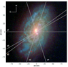 |
Fig. 1. Slit position for the five epochs (e1–e5) of observation over an OSN image of NGC 4414. All slits are centered on SN 2021J. The position of SN 1974G is marked with a red + sign. The image shows a foreground star 5″ SW apart of SN 2021J. |
Information on the OSIRIS/GTC spectroscopy of SN 2021J.
We performed the reduction of the spectra using IRAF standard tasks (Tody et al. 1986), and GTCMOS pipeline (Gómez-González et al. 2016). The full details of the data reduction and its analysis will be presented in a subsequent publication. Here we present a brief summary. Bias and flat-field corrections were applied to the object and standard images. The 2D spectra were calibrated in wavelength using the HgAr+Ne+Xe lamps from the GTC instrument calibration module. The 1D spectra were extracted using an optimal extraction aperture, and the flux calibration was done using spectro-photometric standard stars, observed the same night and with the same gratings than SN 2021J. The atmospheric extinction was corrected using the ORM extinction curve at the observed airmass. The dust extinction in the host galaxy of SN 2021J has not been corrected. The spectra over the different wavelength ranges were combined into a single spectrum for each epoch, and corrected from foreground Galactic reddening (Schlegel et al. 1998).
The SN 2021J spectroscopic evolution over the five epochs is shown in Fig. 2. The strongest early-time features, seen prior to and near the peak brightness, are the Mg II, S II, Si II, and Ca II lines, which are typically observed in type-Ia SNe at similar epochs (Gal-Yam 2017). The late nebular spectrum (day 163 after the peak) shows typical forbidden emission lines of [Fe III] and [Co III] that are generally observed at these late epochs of the SN explosion. The spectra are made publicly available on WISeREP5 (Yaron & Gal-Yam 2012). A detailed analysis of the spectral series of SN 2021J will be presented elsewhere.
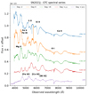 |
Fig. 2. Spectroscopic evolution of SN 2021J over the five epochs observed with OSIRIS/GTC. Each epoch (days from peak brightness) is plotted with a different color. Flux offset for each epoch are reported on the right end of each spectrum. The main line features are also reported, showing the type-Ia nature for SN 2021J. |
3. Analysis
3.1. The light curves of SN 1974G and SN 2021J
The SNe light curves were fitted with the SNooPy (SuperNovae in object oriented Python) package (Burns et al. 2010). The software generates uBVgriYJH light-curve templates to perform a LC fitting to determine the main luminosity parameters. We parameterized the SNe LCs using the decay-rate parameter Δm15 introduced by Phillips (1993), and defined as the difference in magnitude between the peak and 15 days after peak of SN emission in the B band. We selected the max-model implemented in SNooPy for the fits to determine in each filter the maximum magnitude and Δm15. This model does not assume any intrinsic extinction of the SN, neither in the host galaxy nor in the intergalactic medium. The model only corrects for the Milky Way extinction using the Schlegel maps (Schlegel et al. 1998), and it uses the spectral template of Hsiao et al. (2007) to compute K-corrections6. We considered a value of cz = 991 km s−1 for the recessional velocity of NGC 4414 with respect to the CMB rest frame7 (Carrick et al. 2015).
Table 2 shows the LC parameters for both SNe. The first four rows correspond to the maximum brightness in the different filters. We note that SN 1974G has photometric data only in B and V bands. The fifth row indicates the MJD day of B-maximum, and the last row shows the decay-rate parameter. Figure 3 shows the LCs fits for SN 1974G and SN 2021J, respectively. The solid black lines are SNooPy fits for the different filters. Dashed lines in LC fits indicate the 1-σ errors.
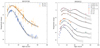 |
Fig. 3. LC fits of the siblings using SNooPy. Left: SN 1974G LCs fits. The orange and blue points correspond to the B- and V-band data taken from Schaefer (1998). The black lines indicate the SNooPy best-fits. Dashed lines are 1-σ errors. Right: SN 2021J LCs fits. The photometry data are obtained from the OSN and Swift. The legend indicates the color and shape of the symbols adopted for the different bands. The black lines indicate the SNooPy best-fits. Dashed lines are 1-σ errors. |
SNooPy best-fit parameters for the LCs of SN 1974G and SN 2021J.
3.2. The Hubble constant
In order to measure the Hubble constant using these two sibling SNe in NGC 4414 as calibrators, we followed the procedure described in Khetan et al. (2021, hereafter K21).
First, we modeled the observed B magnitudes at their maximum based on the main luminosity parameters for type-Ia SNe, including two terms: one provided by Phillips (1993) relating the peak luminosity of a SN Ia and the LC shape, and the other provided by Tripp (1998) including the color correction (see more details in K21). To calibrate the model, here, we used SN 1974G and SN 2021J in the galaxy NGC 4414 with its distance modulus measured from Cepheid variables. By using △m15 to shape the LCs, instead of the color-stretch used in K21, the observed B magnitude at peak is:
 (1)
(1)
where P0 and P1 relate the maximum magnitude to the decay-rate parameter Δm15, R includes the extinction correction that covers other possible causes of reddening, in addition to the galactic extinction that was already taken into account in the LC fitting. We note that our cosmological analysis does not require distinguishing between the different sources of extinction because our goal is not to study the properties of the dust in detail. (Bmax − Vmax) is the pseudo-color defined by the difference between the maximum flux in B and V bands, and μcalib is the distance modulus of the host galaxy.
Several difficulties such as the galaxy compact size, its high surface brightness and a strong source crowding made the study of the Cepheids in NGC 4414 one of the most challenging in the HST Key Project. We adopted the distance modulus of μNGC 4414 = 31.24 ± 0.05 (stat.) mag, as provided in the final results work of the Key Project (Freedman et al. 2001). They improved the value obtained by Turner et al. (1998) and Gibson et al. (2000) by including new corrections in the distance modulus to the Large Magellanic Cloud (LMC), new Wide Field and Planetary Camera 2 (WFPC2) photometric calibration, and improved corrections for metallicity and reddening on the observed period-luminosity (PL) relation of the Cepheids. We used μLMC = 18.477 ± 0.004 (stat.) ±0.026 (syst.) mag recently obtained from an analysis of detached eclipsing binary stars (Pietrzyński et al. 2019) instead of μLMC = 18.50 mag adopted by Freedman et al. (2001).
Second, we used the same cosmological sample as K21, composed of 96 SNe extracted from the Combined Pantheon Sample (Scolnic et al. 2018). We did not apply an upper limit to the SN redshifts, but we selected those SNe from the subsample with good quality photometric data that allows us to adequately sample the LC (see more details in K21). The final redshift range of the sample is 0.02 < z< 0.075. The lower z cut was selected to minimize impact of peculiar velocities uncertainties. We performed a hyerarchical Bayesian regression to infer the model parameters from a likelihood function of the cosmological SN sample, and the two siblings SNe, acting as calibrator sample. Following the methodology by K21, the posterior of the model parameters is given by Bayes’ theorem as
 (2)
(2)
In our study, the LC fit parameters Bmax, Vmax, and Δm15 corresponding to the observable SN properties are included in the vector D, and the model parameters P0, P1, R, H0 are represented by the vector Θ. Their Eq. (6) gives the likelihood probability distribution P(D|Θ) after marginalising over all Θi, computed for each SN, that incorporated the two calibrators and the cosmological sample. In our case, Ncalib = 2 and μcalib = μNGC 4414. We used their Eq. (4) for the SNe cosmological sample to substitute the distance modulus in Eq. (1) as a function of redshift and H0. They considered a cosmological model with a Robertson-Walker metric and a spatially flat Universe (Weinberg 1972; Visser 2005). The values for cosmic deceleration and cosmic jerk are q0 = −0.55 and j0 = 1, respectively (Planck Collaboration VI 2020). In order to derive H0, we consider a hierarchical Bayesian approach consisting of two sub-models, one for the SNe cosmological sample and another for the two sibling SNe in NGC 4414. The variance for each of the two SNe is:
 (3)
(3)
We used Eq. (11) in K21 to calculate the variance of each SN in the cosmological sample. This equation includes the term σint, cosmo which accounts for any unknown scatter in the sample. For the priors, we considered a Half Cauchy distribution for σint, cosmo and normal distributions for the rest of the parameters. We obtained the best-fit parameters of the model P0, P1, R, H0, and σint, cosmo by performing a Markov chain Monte Carlo (MCMC) sampling implemented in Python with the PyMC3 probabilistic programming framework (Salvatier et al. 2016). Figure 4 shows the posterior probability distribution (PPD) of the parameters inferred with the No-U-Turn Sampler (NUTS) algorithm8. Table 3 shows the mean PPD values for the parameters using the two SNe as calibrators in our analysis, separately and together.
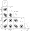 |
Fig. 4. Corner plot showing the posterior probability distributions of the parameters P0, P1, R, H0 and σint, cosmo. The median values of the posterior distributions are displayed on the histograms for each model parameter. |
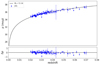 |
Fig. 5. Hubble diagram for the cosmological sample of 96 SNe extracted from the Combined Pantheon Sample (CPS) and calibrated using the two sibling type-Ia SNe. The black line represents the resulting best-fit model. Lower panel residuals from the model fit. |
Posterior probability of the modeling parameters.
We adopted the systematic uncertainties in H0 described in Freedman et al. (2001), but following the updated and improved analysis provided in Freedman et al. (2012) (see more details in Appendix A). We estimated the total systematic error in H0 by adding in quadrature the systematic errors related to the distance modulus to NGC 4414 and those from the fits to the SNe light curves (see Table A.1). After taking into account all the sources of uncertainties, the estimated value of H0 from the two sibling SNe in NGC 4414 is 72.19 ± 2.32 (stat.) ±3.42 (syst.) km s−1 Mpc−1. Although the systematic error is larger than the statistical error in our measurement, it can be reduced in the future, as we argue in Sect. 4. Table 3 also provides the Hubble constant estimates using each of the two SNe separately as calibrators, and compares with the H0 for SN 1974 from the literature.
4. Discussion and conclusions
In this study, we revisit the LC analysis of the known type-Ia SN 1974G in the nearby galaxy NGC 4414. This single calibrator yields a value of the Hubble constant H0 = 70.19 ± 3.32 (stat.) km s−1 Mpc−1, as presented in Sect. 3.2. We obtain a more accurate and precise value of H0, as compared to the significantly lower estimates reported in the literature (see Table 3), by introducing important improvements in our analysis. First, we improved the methodology by applying the SNooPy LC fitter to determine more accurately the LC parameters for all SNe Ia in the cosmological sample and the two sibling SNe in NGC 4414 (SN 1974G and the recently discovered SN 2021J). Secondly, we constructed the Hubble diagram using our sibling SNe (together and separately) as the zero-point calibrators. We used a distant SNe Ia sample extracted from the Combined Pantheon Sample, in the redshift range z = 0.02 − 0.075, instead of using the Calán-Tololo (Hamuy et al. 1996) considered in those SN 1974G previous works. Our cosmological sample is of higher quality and has a larger number of SNe compared with the Calán-Tololo sample (96 vs. 29), which improves the statistical uncertainties in the H0 estimates.
In addition to SN 1974G, we used a recent supernova SN 2021J in the same galaxy as a calibrator. These “siblings” offer additional advantages by sharing several sources of systematics that in general have a non-negligible weight in the estimation of the distance, and then in the calibration of the luminosity relations of the SN. Among these, we have not only the same host distance, but also the peculiar velocity, and host galaxy properties that can have an influence on the luminosity, such as the extinction. However, while Scolnic et al. (2021) find correlations in some SN properties for SNe hosted in the same galaxy, such as the stretch parameter, they do not find greater correlation in the distance modulus values computed by siblings than in any other SN pairs.
Therefore, we have significantly reduced the statistical uncertainties, down to 3.2%, in the determination of H0 from the two sibling SNe in NGC 4414. However, our estimate of H0 = 72.19 ± 2.32 (stat.) ±3.42 (syst.) km s−1 Mpc−1 still has large systematic errors in determining the distance modulus to NGC 4414, as explained in Sect. 3.2. We believe that a new Milky Way Cepheid PL calibration using the upcoming Gaia DR4, together with additional Cepheids from new HST observations, will significantly improve the systematic error of the NGC 4414 distance modulus, and hence provide an accurate determination of H0 at the level of the statistical error.
We have also explored the possibility of measuring the distance modulus to NGC 4414 using the Tip of the Red Giant Branch (TRGB) method. Considering that there are no deep images sampling the stellar halo of the galaxy in the HST archive, it does not seem possible to estimate a distance with this method (Barry Madore, Wendy Freedman, private communications). NGC 4414 may be a good target for the upcoming James Webb space telescope (JWST).
Our estimate of the Hubble constant from the two sibling SNe in NGC 4414 is consistent, within ∼ 1σ with that obtained from early-universe CMB measurements (Planck Collaboration VI 2020) and local estimates from Cepheid variables (Riess et al. 2022; Brout et al. 2022), TRGBs (Freedman 2021), and SBF (K21). Before requiring additional new physics beyond the standard cosmological model, it is imperative to further study possible systematic errors and provide more reliable measurements of H0 using different methodologies in the local Universe. The possibility of finding at least three more pairs of sibling SNe Ia in galaxies with Cepheid distances would not be negligible in the next decade. The ZTF survey (Bellm et al. 2019) discoveries reinforce the previous premise, reporting 1–2 SNe Ia every year in the 20 Mpc volume (Dhawan et al. 2022), where HST observations can provide robust distance estimates by means of Cepheids or TRGB. As a back-of-the-envelope calculation, this means reducing the statistical error of H0 down to 1.7%, similar to what is expected from the entire sample of SNe Ia, and more importantly, it would strongly reduce the systematic error, given that it mainly depends on the uncertainty on the distance modulus of a small number of host galaxies. We finally recall that the systematic error of H0 using these sibling SNe also represents an upper limit since it will be greatly reduced using the incoming Gaia calibrations.
Λ cold dark matter model, where Λ represents the cosmological constant.
Python Software Foundation. Python Language Reference, version 3.9. Available at http://www.python.org
For further information, see https://csp.obs.carnegiescience.edu/data/snpy/documentation
From Cosmic flow model of our local Universe website. For more information see https://cosmicflows.iap.fr/
See more information in https://docs.pymc.io/en/v3/
Acknowledgments
We thank the anonymous referee for the helpful comments. We thank Barry Madore, Wendy Freedman, Radek Wojtak, Eoin Ó Colgáin, and Adam G. Riess for useful comments and discussions. The authors acknowledge financial support from the State Agency for Research of the Spanish MICINN through the “Center of Excellence Severo Ochoa” award to the Instituto de Astrofísica de Andalucía (SEV-2017-0709). EGC thanks the incentive grant by the Ministry of Economic Transformation, Industry, Knowledge and Universities REF. P20_00880, project co-financed by 80% by funds from the operational program FEDER de Andalucía 2014–2020. LI and NK were supported by two grants from VILLUM FONDEN (project number 16599 and 25501). CDT, FP and EP thank the support of the Spanish Ministry of Science and Innovation funding grant PGC2018-101931-B-I00. CDT thanks the Instituto de Astrofísica de Canarias for the use of its facilities to carry out this work. Based on observations collected at the Observatorio de Sierra Nevada, operated by the Instituto de Astrofísica de Andalucía (IAA-CSIC). Partly based on observations made with the Gran Telescopio Canarias (GTC), installed at the Spanish Observatorio del Roque de los Muchachos of the Instituto de Astrofísica de Canarias, in the island of La Palma. The authors thank the GTC support staff for performing the observations.
References
- Bellm, E. C., Kulkarni, S. R., Graham, M. J., et al. 2019, PASP, 131 [Google Scholar]
- Bertin, E., Mellier, Y., Radovich, M., et al. 2002, in Astronomical Data Analysis Software and Systems XI, eds. D. A. Bohlender, D. Durand, & T. H. Handley, ASP Conf. Ser., 281, 228 [NASA ADS] [Google Scholar]
- Biswas, R., Goobar, A., Dhawan, S., et al. 2022, MNRAS, 509, 5340 [Google Scholar]
- Braine, J., Brouillet, N., & Baudry, A. 1997, A&A, 318, 19 [NASA ADS] [Google Scholar]
- Breeveld, A. A., Curran, P. A., Hoversten, E. A., et al. 2010, MNRAS, 406, 1687 [NASA ADS] [Google Scholar]
- Brout, D., Scolnic, D., Popovic, B., et al. 2022, ApJ, submitted [arXiv:2202.04077] [Google Scholar]
- Burns, C. R., Stritzinger, M., Phillips, M., et al. 2010, AJ, 141, 19 [Google Scholar]
- Burns, C. R., Stritzinger, M., Phillips, M. M., et al. 2014, ApJ, 789, 32 [Google Scholar]
- Burns, C. R., Ashall, C., Contreras, C., et al. 2020, ApJ, 895, 118 [NASA ADS] [CrossRef] [Google Scholar]
- Carrick, J., Turnbull, S. J., Lavaux, G., & Hudson, M. J. 2015, MNRAS, 450, 317 [Google Scholar]
- Cepa, J., Aguiar, M., Bland-Hawthorn, J., et al. 2003, in Revista Mexicana de Astronomia y Astrofisica Conference Series, eds. J. M. Rodriguez Espinoza, F. Garzon Lopez, & V. Melo Martin, 16, 13 [NASA ADS] [Google Scholar]
- Ciabattari, F., Mazzoni, E., Donati, S., et al. 2013, Central Bur. Elec. Tel., 3557, 1 [NASA ADS] [Google Scholar]
- Craig, M., Crawford, S., Seifert, M., et al. 2017, https://doi.org/10.5281/zenodo.1069648 [Google Scholar]
- de Jaeger, T., Galbany, L., González-Gaitán, S., et al. 2020, MNRAS, 495, 4860 [NASA ADS] [CrossRef] [Google Scholar]
- de Jaeger, T., Galbany, L., Riess, A. G., et al. 2022, MNRAS, 514, 4620 [NASA ADS] [CrossRef] [Google Scholar]
- Dhawan, S., Goobar, A., Johansson, J., et al. 2022, ApJ, 934, 185 [NASA ADS] [CrossRef] [Google Scholar]
- Ferrarese, L., Silbermann, N. A., Mould, J. R., et al. 2000, PASP, 112, 177 [NASA ADS] [CrossRef] [Google Scholar]
- Forster, F., Bauer, F. E., Munoz-Arancibia, A., et al. 2021, Tran. Name Server Discov. Rep., 2021, 1 [Google Scholar]
- Freedman, W. L. 2021, ApJ, 919, 16 [NASA ADS] [CrossRef] [Google Scholar]
- Freedman, W. L., Madore, B. F., Gibson, B. K., et al. 2001, ApJ, 553, 47 [Google Scholar]
- Freedman, W. L., Madore, B. F., Scowcroft, V., et al. 2012, ApJ, 758, 24 [Google Scholar]
- Gal-Yam, A. 2017, in Handbook of Supernovae, eds. A. W. Alsabti, & P. Murdi, 195 [CrossRef] [Google Scholar]
- Gerke, J., Kochanek, C., Prieto, J., Stanek, K., & Macri, L. 2011, ApJ, 743, 176 [NASA ADS] [CrossRef] [Google Scholar]
- Gibson, B. K., Stetson, P. B., Freedman, W. L., et al. 2000, ApJ, 529, 723 [NASA ADS] [CrossRef] [Google Scholar]
- Gómez-González, V. M. A., Mayya, Y. D., & Rosa-González, D. 2016, MNRAS, 460, 1555 [Google Scholar]
- Hamuy, M., Maza, J., Phillips, M., et al. 1993, AJ, 106, 2392 [NASA ADS] [CrossRef] [Google Scholar]
- Hamuy, M., Phillips, M., Schommer, R. A., et al. 1996, AJ, 112, 2391 [NASA ADS] [CrossRef] [Google Scholar]
- Hsiao, E., Conley, A., Howell, D., et al. 2007, ApJ, 663, 1187 [NASA ADS] [CrossRef] [Google Scholar]
- Hubble, E. P. 1929, ApJ, 69, 103 [NASA ADS] [CrossRef] [Google Scholar]
- Khetan, N., Izzo, L., Branchesi, M., et al. 2021, A&A, 647, A72 [NASA ADS] [CrossRef] [EDP Sciences] [Google Scholar]
- Peebles, P. 2012, Annu. Rev. Astron. Astrophys., 50, 1 [NASA ADS] [CrossRef] [Google Scholar]
- Phillips, M. M. 1993, ApJ, 413, L105 [Google Scholar]
- Pietrzyński, G., Graczyk, D., Gallenne, A., et al. 2019, Nature, 567, 200 [Google Scholar]
- Planck Collaboration VI. 2020, A&A, 641, A6 [NASA ADS] [CrossRef] [EDP Sciences] [Google Scholar]
- Prieto, J. L., Rest, A., & Suntzeff, N. B. 2006, ApJ, 647, 501 [NASA ADS] [CrossRef] [Google Scholar]
- Riess, A. G., Press, W. H., & Kirshner, R. P. 1996, ApJ, 473, 88 [Google Scholar]
- Riess, A. G., Macri, L. M., Hoffmann, S. L., et al. 2016, ApJ, 826, 56 [Google Scholar]
- Riess, A. G., Casertano, S., Yuan, W., et al. 2021, ApJ, 908, L6 [NASA ADS] [CrossRef] [Google Scholar]
- Riess, A. G., Yuan, W., Macri, L. M., et al. 2022, ApJ, 934, L7 [NASA ADS] [CrossRef] [Google Scholar]
- Salvatier, J., Wiecki, T. V., & Fonnesbeck, C. 2016, PeerJ Comput. Sci., 2, e55 [Google Scholar]
- Schaefer, B. E. 1998, ApJ, 509, 80 [NASA ADS] [CrossRef] [Google Scholar]
- Schlegel, D. J., Finkbeiner, D. P., & Davis, M. 1998, ApJ, 500, 525 [Google Scholar]
- Scolnic, D. M., Jones, D., Rest, A., et al. 2018, ApJ, 859, 101 [NASA ADS] [CrossRef] [Google Scholar]
- Scolnic, D., Smith, M., Massiah, A., et al. 2020, ApJ, 896, L13 [NASA ADS] [CrossRef] [Google Scholar]
- Scolnic, D., Brout, D., Carr, A., et al. 2021, ApJ, submitted [arXiv:2112.03863] [Google Scholar]
- Tody, D. 1986, in Instrumentation in astronomy VI, ed. D. L. Crawford, SPIE Conf. Ser., 627, 733 [Google Scholar]
- Tripp, R. D. 1998, A&A, 331, 815 [NASA ADS] [Google Scholar]
- Tripp, R. 1998, A&A, 331, 815 [NASA ADS] [Google Scholar]
- Turner, A., Ferrarese, L., Saha, A., et al. 1998, ApJ, 505, 207 [NASA ADS] [CrossRef] [Google Scholar]
- Van Dyk, S. D., Zheng, W., Fox, O. D., et al. 2014, AJ, 147, 37 [Google Scholar]
- Verde, L., Treu, T., & Riess, A. G. 2019, Tensions between the early and late Universe (Nature Publishing Group) [Google Scholar]
- Visser, M. 2005, Gen. Relativ. Gravit., 37, 1541 [CrossRef] [Google Scholar]
- Weinberg, S. 1972, Gravitation and cosmology: principles and applications of the general theory of relativity [Google Scholar]
- Yaron, O., & Gal-Yam, A. 2012, PASP, 124, 668 [Google Scholar]
Appendix A: Systematic uncertainties on the Hubble constant
We adopted the systematic uncertainties in H0 described in Freedman et al. (2001) and Freedman et al. (2012), who provided the Cepheid distance to NGC 4414 used in this study. The former detected Cepheid variables and derived accurate distances to nearby SN Ia hosts, including NGC 4414. The latter focused mainly on the zero point of the Cepheid extragalactic distance scale and a re-evaluation of the systematic error budget, and hence improving the systematic errors.
We show in Table A.1 the systematic error budget on H0 (see more details in Freedman et al. 2012). The systematics of the SNooPy fits were obtained in this work. The total error in H0 was then calculated by combining all the individual errors in quadrature. The choice of the uncertainty in the metallicity parameter is controversial due to the value adopted for the Cepheid metallicity coefficient (see Fig. 14 in Gerke et al. 2011). Although there are works with smaller values (e.g. Riess et al. 2021), we conservatively considered the 4% error adopted in Freedman et al. (2001), since we used the distance to the galaxy from this work. We adopted a 1% uncertainty due to crowding, as reported in Freedman et al. (2012). They present a quantitative analysis of the crowding bias in Cepheid photometry using artificial stars. The blue main sequence stars are the main contributors to the crowding, which make Cepheid photometry brighter and bluer. The systematic bias closely tracks the line of the Wesenhelt reddening free index (W) in the optical CMD, resulting in a minimal change in the final Cepheid distance (see more details in their Section 3.3 and their Appendix). Freedman et al. (2012) conclude that the crowding effects are less than 0.02 mag (1% in distance), in agreement with the results of Ferrarese et al. (2000). Our estimated value of H0 and its uncertainties from the two sibling SNe in NGC 4414 is 72.19 ± 2.32 (stat.) ±3.42 (syst.) km s−1 Mpc−1.
Budget of systematic errors on H0 from the 2 sibling SNe in NGC 4414
Appendix B: Photometry of SN 2021J
In this section, we report the photometry of SN 2021J. On the one hand, Table B.1 shows BVRI photometry of SN 2021J in eight epochs obtained with the CCDT150 camera mounted on the 1.5m telescope at the Observatorio de Sierra Nevada (OSN). On the other hand, Table B.2 presents UBV photometry observed by Swift-UVOT.
Photometry of SN 2021J obtained with the CCDT150 camera mounted on the 1.5 meter telescope at the OSN.
Photometry of SN 2021J obtained by Swift Ultraviolet/Optical Telescope.
Appendix C: EBV_model2 LC fitting for SN 2021J
As seen previously, we used the max-model in SNooPy to fit the LCs for the SNe, which allowed us to compute the maximum magnitude in each filter and △m15 needed for the Bayesian analysis. In this section, we calculate the LC parameters for SN 2021J by using another fitting model: the EBV_model2. This model allows us to compute the distance and the dust extinction of the host galaxy following the work of Prieto et al. (2006). We parameterized the SNe LCs using the color-stretch parametersBV introduced by Burns et al. (2014) and defined as the time between Bmax and (Bmax − Vmax) divided by 30. We obtained a value of the reddening due to the host galaxy of E(B − V)host = 0.349 ± 0.018 mag, sBV = 0.988 ± 0.024, and μNGC4414 = 30.927 ± 0.053 mag. Figure C.1 shows the LCs fits obtained. Fitting this model to just two filters for SN 1974G is not accurate to correctly disentangle the intrinsic extinction. Therefore, we decided to use the max-model that meets the requirements of our work.
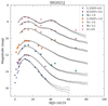 |
Fig. C.1. SN 2021J LCs fits using the EVB_model in SNooPy. The legend indicates the color and shape of the symbols adopted for the different bands. The black lines indicate the SNooPy best-fits. Dashed lines are 1-σ errors. |
Appendix D: Uncertainty analysis of SN 1974G
In this section, we study the uncertainties corresponding to SN 1974G. As we seen in previous sections, we used the B- and V-band photometry of SN 1974G presented in Schaefer (1998). Due to the existing data contains both visual and photographic magnitudes, we studied our results in different cases, depending on what points are included in our analysis. Figure D.1 shows the LCs fits for SN 1974G for the different analysis. The solid black lines are SNooPy fits for the different filters. Dashed lines in LC fits indicate the 1-σ errors. In a) we have considered all the points that Schaefer (1998) adopted. In b) we have removed the visual, photographic, and points with large uncertainty (Burgat’s points, see Table 3 in Schaefer (1998)). In c) we have removed only the visual, and photographic points. Table D.1 shows the LC parameters for SN 1974G. The results are still consistent within the margins of error. Finally, we decided to consider all the original points because the SN peak is better covered. Furthermore, the large uncertainties of SN 1974G are within our luminosity calibration code and reflected in the different weights of the two SNe.
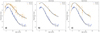 |
Fig. D.1. SN 1974G LCs fits using SNooPy. The black lines indicate the SNooPy best-fits. Dashed lines are 1-σ errors. (a) Considering all the point used by Schaefer (1998). (b) Eliminating the visual, photographic, and Burgat’s points. (c) Eliminating the visual, and photographic points. |
SNooPy best-fit parameters for the LCs of SN 1974G. (a) Considering all the point used by Schaefer (1998). (b) Eliminating the visual, photographic, and Burgat’s points. (c) Eliminating the visual, and photographic points.
All Tables
Photometry of SN 2021J obtained with the CCDT150 camera mounted on the 1.5 meter telescope at the OSN.
SNooPy best-fit parameters for the LCs of SN 1974G. (a) Considering all the point used by Schaefer (1998). (b) Eliminating the visual, photographic, and Burgat’s points. (c) Eliminating the visual, and photographic points.
All Figures
|
Fig. 1. Slit position for the five epochs (e1–e5) of observation over an OSN image of NGC 4414. All slits are centered on SN 2021J. The position of SN 1974G is marked with a red + sign. The image shows a foreground star 5″ SW apart of SN 2021J. |
| In the text | |
|
Fig. 2. Spectroscopic evolution of SN 2021J over the five epochs observed with OSIRIS/GTC. Each epoch (days from peak brightness) is plotted with a different color. Flux offset for each epoch are reported on the right end of each spectrum. The main line features are also reported, showing the type-Ia nature for SN 2021J. |
| In the text | |
|
Fig. 3. LC fits of the siblings using SNooPy. Left: SN 1974G LCs fits. The orange and blue points correspond to the B- and V-band data taken from Schaefer (1998). The black lines indicate the SNooPy best-fits. Dashed lines are 1-σ errors. Right: SN 2021J LCs fits. The photometry data are obtained from the OSN and Swift. The legend indicates the color and shape of the symbols adopted for the different bands. The black lines indicate the SNooPy best-fits. Dashed lines are 1-σ errors. |
| In the text | |
|
Fig. 4. Corner plot showing the posterior probability distributions of the parameters P0, P1, R, H0 and σint, cosmo. The median values of the posterior distributions are displayed on the histograms for each model parameter. |
| In the text | |
|
Fig. 5. Hubble diagram for the cosmological sample of 96 SNe extracted from the Combined Pantheon Sample (CPS) and calibrated using the two sibling type-Ia SNe. The black line represents the resulting best-fit model. Lower panel residuals from the model fit. |
| In the text | |
|
Fig. C.1. SN 2021J LCs fits using the EVB_model in SNooPy. The legend indicates the color and shape of the symbols adopted for the different bands. The black lines indicate the SNooPy best-fits. Dashed lines are 1-σ errors. |
| In the text | |
|
Fig. D.1. SN 1974G LCs fits using SNooPy. The black lines indicate the SNooPy best-fits. Dashed lines are 1-σ errors. (a) Considering all the point used by Schaefer (1998). (b) Eliminating the visual, photographic, and Burgat’s points. (c) Eliminating the visual, and photographic points. |
| In the text | |
Current usage metrics show cumulative count of Article Views (full-text article views including HTML views, PDF and ePub downloads, according to the available data) and Abstracts Views on Vision4Press platform.
Data correspond to usage on the plateform after 2015. The current usage metrics is available 48-96 hours after online publication and is updated daily on week days.
Initial download of the metrics may take a while.