| Issue |
A&A
Volume 698, June 2025
|
|
|---|---|---|
| Article Number | A222 | |
| Number of page(s) | 12 | |
| Section | Numerical methods and codes | |
| DOI | https://doi.org/10.1051/0004-6361/202553751 | |
| Published online | 20 June 2025 | |
Estimation of age and metallicity for galaxies based on multi-modal deep learning
1
School of Computer and Information, Dezhou University,
Dezhou
253023,
China
2
School of Information and Control Engineering, Jilin Institute of Chemical Technology,
Jilin
132022,
China
3
International Centre of Supernovae, Yunnan Key Laboratory,
Kunming
650216,
China
★ Corresponding author: This email address is being protected from spambots. You need JavaScript enabled to view it.
Received:
14
January
2025
Accepted:
22
April
2025
Abstract
Aims. This study is aimed at deriving the age and metallicity of galaxies by proposing a novel multi-modal deep learning framework. This multi-modal framework integrates spectral and photometric data, offering advantages in cases where spectra are incomplete or unavailable.
Methods. We propose a multi-modal learning method for estimating the age and metallicity of galaxies (MMLforGalAM). This method uses two modalities: spectra and photometric images as training samples. Its architecture consists of four models: a spectral feature extraction model (ℳ1), a simulated spectral feature generation model (ℳ2), an image feature extraction model (ℳ3), and a multi-modal attention regression model (ℳ4). Specifically, ℳ1 extracts spectral features associated with age and metallicity from spectra observed by the Sloan Digital Sky Survey (SDSS). These features are then used as labels to train ℳ2, which generates simulated spectral features for photometric images to address the challenge of missing observed spectra for some images. Overall, ℳ1 and ℳ2 provide a transformation from photometric to spectral features, with the goal of constructing a spectral representation of data pairs (photometric and spectral features) for multi-modal learning. Once ℳ2 is trained, MMLforGalAM can then be applied to scenarios with only images, even in the absence of spectra. Then, ℳ3 processes SDSS photometric images to extract features related to age and metallicity. Finally, ℳ4 combines the simulated spectral features from ℳ2 with the extracted image features from ℳ3 to predict the age and metallicity of galaxies.
Results. Trained on 36278 galaxies from SDSS, our model predicts the stellar age and metallicity, with a scatter of 1σ = 0.1506 dex for age and 1 σ = 0.1402 dex for metallicity. Compared to a single-modal model trained using only images, the multi-modal approach reduces the scatter by 27% for age and 15% for metallicity.
Key words: methods: data analysis / methods: statistical / techniques: photometric / surveys
© The Authors 2025
 Open Access article, published by EDP Sciences, under the terms of the Creative Commons Attribution License (https://creativecommons.org/licenses/by/4.0), which permits unrestricted use, distribution, and reproduction in any medium, provided the original work is properly cited.
This article is published in open access under the Subscribe to Open model. This email address is being protected from spambots. You need JavaScript enabled to view it. to support open access publication.
1 Introduction
Galaxies are systems of stars, gas, dust, and dark matter that evolve over cosmic timescales. Stellar age and metallicity are key parameters indicating a galaxy’s evolutionary history and the processes shaping it (Kennicutt 1998). Stellar age reveals the history of star formation within a galaxy and reflects episodes of active and quiescent star birth. Meanwhile, metallicity, defined as the abundance of elements heavier than hydrogen and helium, indicates the chemical enrichment of both the interstellar gas and the stars within a galaxy (Gallazzi et al. 2005; Gallazzi et al. 2006). Therefore, accurate estimations of stellar age and metallicity provide insights into the chemical evolution and star formation history of galaxies.
Traditional methods for measuring age and metallicity of galaxies, such as stellar population synthesis (SPS), generally rely on comparing observed spectra of galaxies with theoretical simulations. SPS involves creating models that simulate the combined light of a stellar population. By varying the parameters of these models, such as the ages, metallicities, and masses of the stars, researchers can generate template spectra, which can then be compared with observed spectra to estimate the properties and evolutionary history of these galaxies (Bruzual & Charlot 2003; Maraston 2005; Vazdekis et al. 2010; Maraston & Strömbäck 2011; Vazdekis et al. 2016). Over the past two decades, several full-spectrum fitting tools have used SPS models to analyse spectra and estimate various physical parameters of galaxies, such as pPXF (Cappellari & Emsellem 2004; Cappellari 2017, 2023), STARLIGHT (Cid Fernandes et al. 2005), STECKMAP (Ocvirk et al. 2006), VESPA (Tojeiro et al. 2007), FIREFLY (Wilkinson et al. 2015, 2017), BEAGLE (Chevallard & Charlot 2016), and FADO (Gomes & Papaderos 2017). These algorithms apply fullspectrum information during χ2 minimization to match observed spectra with template spectra. While the methods of SPS offer high precision, they are computationally intensive and timeconsuming, particularly when processing large datasets that require extensive iterative calculations (Wang et al. 2022).
With the growing number of large-scale astronomical surveys, including Sloan Digital Sky Survey (SDSS; York et al. 2000), Large Sky Area Multi-Object Fiber Spectroscopic Telescope (LAMOST; Cui et al. 2012; Luo et al. 2015), Euclid (Laureijs et al. 2011; Euclid Collaboration: Mellier et al. 2025), Large Synoptic Survey Telescope (LSST; LSST Science Collaboration 2009; LSST Dark Energy Science Collaboration 2012) and Dark Energy Spectroscopic Instrument (DESI; Dey et al. 2019), the volume of available astronomical data has increased substantially. Machine learning (ML) and deep learning (DL) provide effective tools for processing these vast datasets by automatically extracting complex features from highdimensional data. In astronomy, ML and DL have shown good performance in estimating galaxy physical parameters using either spectra (Bonjean et al. 2019; Surana et al. 2020; Liew-Cain et al. 2021; Zeraatgari et al. 2024; Wang et al. 2024; Wu et al. 2024) or photometric images (Hoyle 2016; Wu & Boada 2019; Henghes et al. 2022; Zhong et al. 2024). For example, in our previous work (Wang et al. 2024), we applied SDSS spectra to train a deep learning model for predicting galaxy stellar population properties, including age, metallicity, colour excess, and central velocity dispersion. Wu et al. (2024) used a one-dimensional deep convolutional neural network (CNN), GalSpecNet, to classify galaxy spectra from SDSS and LAMOST into star-forming, composite, active galactic nucleus (AGNs), and normal types, achieving an accuracy of over 94% and releasing a catalogue of 96000 classified galaxies. For photometric images, Wu & Boada (2019) used deep convolutional neural networks (CNNs) to predict galaxy gas-phase metallicity from SDSS three-colour (GRB) images, achieving a root mean square error (RMSE) of 0.085 dex. Zhong et al. (2024) proposed the Galaxy Efficient Network (GalEffNet) deep learning model that uses photometric images from DESI to estimate stellar mass ( M* ) and specific star formation rate (SSFR) of galaxies. Their GalEffNet demonstrates good performance with standard deviations of 0.218 dex for M* and 0.410 dex for sSFR. Despite these advances, most ML or DL methods rely on single-modal data, either spectra or images. Multi-modal learning, which integrates multiple data sources, has the potential to improve parameter estimation. Therefore, in this study, we aim to develop a multi-modal deep learning model that combines spectra and photometric images to estimate stellar age and metallicity in galaxies.
Recently, multi-modal research has started to gain attention in astronomy. Integrating diverse data modalities, such as photometric images, spectra, and metadata, has significantly advanced tasks such as classification, redshift prediction, and parameter estimation. For example, Parker et al. (2024) proposed the cross-modal self-supervised model AstroCLIP, which combines galaxy image and spectral data to enable tasks such as morphology classification and photometric redshift estimation. Hong et al. (2023) utilised spectra and photometric images to enhance photometric redshift estimation. Gai et al. (2024) proposed the FusionNetwork model, which integrates H-band imaging data and photometric images to estimate galaxy redshifts, stellar mass, and star formation rates. These studies demonstrate that integrating multi-modal data has advanced astronomical classification and prediction, enabling more effective large-scale multi-modal data analysis.
In this work, we propose a multi-modal learning approach for inferring age and metallicity of galaxies (MMLforGalAM). This multi-modal framework combines spectra and photometric images to achieve a more comprehensive feature representation of galaxy properties, consequently improving prediction accuracy in comparison with models trained using only photometric images. The structure of this paper is as follows. Section 2 provides details on the data selection, acquisition, and pre-processing. In Sect. 3, we introduce the proposed method and model architecture. Section 4 presents the experiments to evaluate the performance of our model. Finally, Sect. 5 summarises the paper.
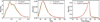 |
Fig. 1 Comparison of the redshift, S/N, and magnitude (petroMag_r) distributions between the randomly selected sample and the full dataset. |
2 Data
This section describes the dataset used in this study, which comprises two modalities: spectra and images, as well as their pre-processing steps.
2.1 Multi-modal dataset
The MMLforGalAM is trained on a dataset consisting of galaxy images and their corresponding spectra from the SDSS.
2.1.1 Spectra
The spectra used in this work are sourced from SDSS Data Release 7 (DR7). There are about 930000 galaxy spectra in SDSS DR7. These spectra cover a wavelength range from 3800 to 9200Å and have a spectral resolution of R∼2000. We selected some spectra from SDSS DR7 for model training in this work, using selection criteria consistent with our previous work (Wang et al. 2024):
0.002 ≤ z ≤ 0.3 and zWarning = 0. The chosen redshift range1 ensures that key spectral lines, such as Hβ, Mg, Na, and Hα, fall within the observed wavelength range, which is essential for estimating stellar populations. Also, zWarning = 0 indicates that the redshifts of selected galaxies are reliable.
S/N ≥ 5, where S/N is the signal-to-noise ratio in the r-band. This criterion excludes low-quality data from the dataset.
Applying the above selection criteria, about 800000 spectra are obtained. To alleviate computational demands, 50000 spectra are randomly selected for further analysis. Figure 1 illustrates the distributions of redshift, S/N, and r-band magnitude (petro-Mag_r; Petrosian 1976) in both the selected sample and the full dataset. It is observed that the distribution of the randomly selected sample is consistent with that of the full dataset. For redshift, most values in both samples are within the range [0.05, 0.2 ]. The S/N is primarily distributed in the range [10, 30], while most PetroMag_r values lie between 16 and 18.
The prediction of age and metallicity is treated as supervised learning. To obtain the ground truth values for these parameters, we employ a traditional full-spectrum fitting method pPXF (Cappellari & Emsellem 2004; Cappellari 2017, 2023), following the methodology outlined in our previous work (Wang et al. 2024). Specifically, we use pPXF with 36 simple stellar population (SSP) templates from Vazdekis et al. (2010), which contains nine ages (0.06, 0.12, 0.25, 0.5, 1.0, 2.0, 4.0, 8.0, and 15 Gyr ) and four metallicity (−1.71,−0.71,0, and 0.22 in log (Z/Z⊙)). These templates are then re-binned to the same velocity scale of the SDSS galaxy spectrum and convolved with the quadratic difference between the instrumental resolutions of SDSS and templates. We fit the normalised spectra in our sample to these templates to derive the luminosity-weighted average age and metallicity used as the ground truth.
2.1.2 Photometric images
We use the JPEG version of the SDSS images, which are retrieved and constructed by the ImgCutout web service by querying the Catalogue Archive Server (CAS) database. These JPEG images are generated by the FITS2JPEG converter2, which converts the g, r, and i-band FITS images into three-colour JPEG images, mapping i, r, and g bands to the R, G, and B channels, respectively. The converted images are then stored in the CAS database for direct access.
To download the SDSS JPEG-images corresponding to our spectra, we use the SDSS ImgCutout service3, which extracts images from the CAS database, based on given right ascension (RA) and declination (Dec). The service locates the relevant JPEG image, trims it to the specified width and height, and ensures that the requested coordinates are centered within the extracted image. In this work, we set the width and height of the image cut to 128 pixels in the ImgCutout service, while additional image resolution for comparison is detailed in Appendix A. Figure 2 presents some examples of photometric images and spectra of galaxies with different S/Ns. The upperright corner of each spectrum displays the corresponding galaxy RA, Dec, redshift, and S/N.
Through these steps, a total of 50000 pairs of spectra and photometric images are collected for subsequent analysis. As mentioned previously, these images are the gri-band combination provided by the SDSS ImgCutout service. The influence of different filter bands on model performance is described in Appendix A.
2.2 Data pre-processing
After selecting and preparing the dataset, the following subsections describe the pre-processing methods applied to spectra and photometric images.
2.2.1 Pre-processing of spectra
Spectral pre-processing includes resampling and normalisation. The specific steps are outlined below:
Resampling: each spectrum is resampled at 1Å intervals within the 3830−8000 Å range to ensure consistent dimensionality: 1030 spectra are excluded because they fall outside this range.
-
Min—max normalisation: the min—max normalisation is applied according to Eq. (1):
 (1)
(1)where X represents the original data points, and Xmin and Xmax are the minimum and maximum values of the spectrum, respectively. The normalised data points are denoted as Xnorm.
After pre-processing, each spectrum comprises 4171 data points, representing its features.
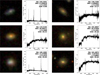 |
Fig. 2 Examples of photometric images and their corresponding spectra with different S/Ns. In each panel, the right ascension (RA) and declination (Dec), redshift, and S/N of the galaxy are given on the upper-right corner. |
2.2.2 Pre-processing of photometric images
This process includes masking noisy astronomical sources, identifying blended galaxies, and cropping the images. The specific pre-processing steps are outlined as follows:
-
Masking noisy astronomical sources: A photometric image often contains multiple celestial objects, but only the galaxy at the centre of the image is considered as the target in our work. Therefore, we first mask the image to retain only the target galaxy using adaptive thresholding and contour fitting techniques (Zhong et al. 2024). The process is as follows. First, each photometric image is individually scaled to the [0,1] range and then converted to greyscale. Next, an initial threshold of image segmentation is set based on the maximum and minimum greyscale values. This threshold is iteratively refined based on foreground and background averages until convergence. Subsequently, the final threshold generates a binary segmentation image by extracting regions with grayscale values above it. During the contour fitting, an edge detection is applied to the binary image to extract galaxy contours, and ellipses are fitted to these contours using OpenCV4. Finally, the fitted ellipse at the centre of the image is determined as the target galaxy, with regions outside the ellipse masked in black.
This OpenCV-based elliptical fitting method may introduce certain biases in complex environments, such as disturbed galaxies, and low-surface-brightness galaxies, similar to the issues discussed in Appendix A.2 of Zhong et al. (2024). On some images, the algorithm fails to accurately identify the target galaxy at the centre of the images or properly fit their contours. The images of these galaxies will be filtered out. In this work, approximately 0.58% of the photometric images are removed by the masking step.
-
Identifying blended galaxies: Blended galaxies arise when multiple galaxies overlap because of their proximity along the line of sight. This blending obscures surface brightness, shape, and spectral characteristics, making it difficult to determine their properties accurately. To ensure accurate measurements of age and metallicity, blended galaxies have been excluded from this work. We identified blended galaxies using PHOTUTILS5. Because of their connected pixel values, blended galaxies appear as single sources. We utilised PHOTUTILS to detect saddle points between sources to determine whether they are blended. If more than one source was detected within a single location, we then identified the object as a blended galaxy.
To quantitatively assess the effectiveness of the PHOTUTILS blended galaxy detection method, we applied it to a randomly selected sample of 100 blended galaxy images from our dataset. A visual inspection confirmed that 91% of these images are correctly identified as blended galaxies, which demonstrates the algorithm’s effectiveness. And then, this method was applied to our full dataset. As a result, PHOTUTILS was able to identify 25% of the images as blended galaxies. These images were subsequently removed to ensure a cleaner dataset for further analysis.
Cropping images: After masking the noise, the image may contain large black regions at the periphery, which are irrelevant for deep learning. Thus, a central crop is applied to retain only the target galaxy at the centre of the image. The image is then resized to 128 × 128 pixels using nearestneighbour interpolation to avoid introducing artifacts and to preserve pixel intensity relationships during re-scaling.
The complete workflow of the photometric image pre-processing is illustrated in Fig. 3, using two randomly selected examples: one with blended galaxies and one unblended. In panel (a), the original images of blended and unblended galaxies are shown; and in panel (b), the results after masking the noisy sources are displayed; in panel (c), the unblended image is presented after identification and cropping; in panel (d), the blended image is identified and then discarded.
Following the pre-processing procedure detailed here, a dataset of 36278 images paired with their corresponding spectra was ready for the multi-modal learning step.
3 Methodology
This study proposes a multi-modal deep learning (MMLforGalAM) approach that combines spectra and photometric images to improve galaxy age and metallicity estimations. This method is composed of four key models: a spectral feature extraction model (ℳ1), a simulated spectral feature generation model (ℳ2), an image feature extraction model (ℳ3), and a multi-modal attention regression model (ℳ4). The framework of the MMLforGalAM is depicted in Fig. 4.
Spectral feature extraction model (ℳ1): This model extracts key features indicative of galaxy age and metallicity from spectra. These extracted features are then used as training labels for ℳ2. A detailed description of ℳ1 is provided in Sect. 3.1.
Simulated spectral feature generation model (ℳ2): In astronomical observations, many photometric images lack corresponding spectra, resulting in missing spectral information for input into our multi-modal model. To address this issue, the ℳ2 bridges the gap by generating spectral features from photometric images. These simulated spectral features are then used as input for ℳ4. The purpose of ℳ1 and ℳ2 is to construct a spectral representation of data pairs (photometric and spectral features), which are necessary for multi-modal learning. Further details of ℳ2 are presented in Sect. 3.2.
Image feature extraction model (ℳ3) : this model extracts features from galaxy images that correlate with galaxy age and metallicity. There are two goals of this model: (1) to estimate the galaxy age and metallicity using images alone, to enable comparison with multi-modal estimation from ℳ4, and (2) to provide image features as input for ℳ4. Detailed information is provided in Sect. 3.3.
Multi-modal attention regression model (ℳ4): this model integrates features from both the simulated spectra and images.
Through an attention mechanism, this model adjusts feature weights to enhance the accuracy of galaxy parameter predictions. Further details are provided in Sect. 3.4.
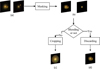 |
Fig. 3 Workflow of photometric image pre-processing: (a) shows the original images of blended and unblended galaxies; (b) displays the images after masking noisy sources; (c) presents the unblended image after identification and cropping; (d) shows the blended image, which has been discarded. |
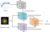 |
Fig. 4 Framework of the MMLforGalAM. |
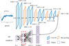 |
Fig. 5 Architecture of the spectral feature extraction model (ℳ1). The shape of each layer is represented as a × b × c or a × b, where a × b represents the feature map dimensions and c is the number of convolutional filters. The red dashed box represents the final fully connected layer, whose output serves as the label for training the next model, ℳ2. |
3.1 Spectral feature extraction model (ℳ1)
The model ℳ1 employs a one-dimensional convolutional neural network (1D CNN) to extract spectral features characterizing the age and metallicity of galaxies. The final fully connected layer of the model, which encodes age and metallicity information, is used as our feature representation. The extracted features then serve as labels for generating simulated spectral features in the model ℳ2.
The architecture of the model is depicted in Fig. 5, consisting of an input layer, convolutional and max-pooling layers, a flatten layer, fully connected layers, and an output layer. Each component is described below:
(1) input layer: the input spectrum to the model consists of 4171 data points;
(2) convolutional and max-pooling layers: the model includes four convolutional blocks, each comprising two convolutional layers. The number of filters in these layers increases across the blocks, with 16, 32, 64, and 128 filters in the first through fourth blocks, respectively. The convolutional layers use a kernel size of 3 with ReLU activation, and max-pooling is applied to reduce the feature map dimensions. L2 regularisation is incorporated to prevent overfitting. In Fig. 5, the shape of each layer is represented as a × b × c or a × b, where a × b denotes the dimensions of the output feature map and c represents the number of convolutional filters;
(3) one flatten layer: the output from the final max-pooling layer is flattened into a one-dimensional vector, serving as input to the fully connected layers;
(4) two fully connected layers: following the flatten layer are two fully connected layers. The final fully connected layer serves as an abstract spectral representation capable of expressing age and metallicity. The output of this layer, highlighted by the red dashed box in Fig. 5, serves as the label for training ℳ2;
(5) output layer: the output layer employs a linear activation function for regression, predicting the age and metallicity of galaxies.
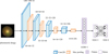 |
Fig. 6 Architecture of the simulated spectral feature generation model (ℳ2). The numbers in the form a × b × c or a × b for each layer are consistent with Fig. 5. |
3.2 Simulated spectral feature generation model (ℳ2)
The primary motivation for including ℳ2 is to create a framework robust to scenarios where there are no available spectra. By training ℳ2 to generate simulated spectral features from photometric images, we can build our MMLforGalAM model with the capability to provide robust age and metallicity estimates even when only images are available, without the corresponding spectra. Specifically, ℳ2 employs a two-dimensional convolutional neural network to learn a transformation from photometric images to spectral features. The model takes photometric images as input, and the labels are spectral features extracted by ℳ1. After training, ℳ2 gains the ability to transform photometric images into simulated spectral features. This transformation addresses the issue of missing corresponding observed spectra for certain photometric images. Therefore, in ℳ4, both image features and the simulated spectral features are used as inputs. The detailed architecture of the model is shown in Fig. 6. The architecture set-up is as follows:
(1) input layer: the model accepts photometric images with a resolution of 128 × 128 pixels as input;
(2) convolutional and max-pooling layers: the network includes four convolutional layers, each with a 3 × 3 convolutional kernel and ReLU activation function. The number of filters in these layers increases progressively, with 32,64,128, and 256 filters. Each convolutional layer is followed by a maxpooling layer with a window size of 2 × 2, which selects the maximum value from each 2 × 2 region of the feature map;
(3) one flatten layer;
(4) one fully connected layer: the features extracted by the fully connected layers serve as representations for the prediction targets;
(5) output layer: the output layer generates a 1024dimensional simulated spectral feature, which is subsequently utilised in multi-modal fusion tasks.
3.3 Image feature extraction model (ℳ3)
The model ℳ3 uses a two-dimensional convolutional neural network to estimate the age and metallicity. The architecture of ℳ3 is illustrated in Fig. 7. As shown in Fig. 7, the red dashed box indicates the extracted image features related to age and metallicity. Each image has a feature dimension of 1024. The architecture is described as follows:
(1) input layer: the input of the model is photometric images with a resolution of 128 × 128 pixels;
(2) convolutional and max-pooling layers: there are four convolutional blocks, each consisting of three convolutional layers followed by a max-pooling layer with a window size of 2 × 2. The number of filters in the convolutional layers increases progressively: 32 filters in the first block, 64 in the second, 128 in the third, and 256 in the fourth. Each convolutional layer uses a 3 × 3 kernel and applies the ReLU activation function. Additionally, L2 regularization is used to prevent overfitting;
(3) one flatten layer;
(4) two fully connected layers: the two fully connected layers learn complex representations of the photometric images. Features from the final fully connected layer serve as the image modality, used as input to the multi-modal model, ℳ4;
(5) output layer: the output layer provides predictions for age and metallicity. We compared these predictions with the outputs of the multi-modal model to demonstrate the advantages of the multi-modal approach over a single-modal model based solely on images.
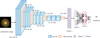 |
Fig. 7 Architecture of the image feature extraction model (ℳ3). The red dashed box highlights the image features related to age and metallicity, which are used as input to the multi-modal model (ℳ4). |
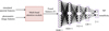 |
Fig. 8 Architecture of the multi-modal attention regression model (ℳ4). |
3.4 Multi-modal attention regression model (ℳ4)
The multi-modal attention regression model (ℳ4) integrates features extracted from both images and spectra using an attention mechanism to optimize feature selection and weighting.
The architecture is illustrated in Fig. 8. ℳ4 employs a multi-head attention mechanism to effectively fuse multi-modal features of images and spectra. These fused features are then processed through a neural network consisting of five fully connected layers, which extract high-level representations for regression predictions of age and metallicity.
The overall architecture of ℳ4 includes the following key components:
(1) input layer: the inputs to this model are simulated spectral features generated by ℳ2 and image features extracted by ℳ3;
(2) multi-modal feature fusion: to effectively integrate spectral and image features, a weighted fusion strategy based on the multi-head attention mechanism (Vaswani 2017) is employed. This mechanism runs multiple attention heads in parallel, allowing the model to capture attention distributions across different subspaces of the input features. The workflow of the multi-head attention module is shown in Fig. 9.
In attention mechanisms, a query (Q), key (K), and value (V) are used to compute a weighted sum of information. The query represents what we are looking for, the keys represent the available information and the values are what we want to extract based on relevance. Specifically, the query is compared against the keys to calculate attention scores and these scores determine the weights for each corresponding value. In our multi-modal model, the spectral features, S, serve as the query because they provide more detailed information for determining age and metallicity, making them ideal for guiding the attention mechanism. The image features, I, act as both the keys and values.
First, S and I are projected into a shared subspace via linear mapping, which makes it easier to compare and combine features from different modalities. The transformation is expressed in Eq. (2):
 (2)
(2)
where WQ, WK, and WV are weight matrices for the query, key, and value, respectively.
Second, we compute the attention weights using the ’scaled dot-product attention’ function (Vaswani 2017), as defined in Eq. (3):
 (3)
(3)
The input of this function consists of queries (Q), keys (K), and values (V). We computed the dot product between the query and all keys, and divided each by the scaling factor  to control the numerical range and ensure stable gradients. This scaled result is called the attention score. These scores are then normalised using the softmax function to obtain attention weights. These weights are used to compute a weighted sum of all values, resulting in the final attention vector.
Third, multiple attention heads are computed to capture different feature subspaces, as shown in Eq. (4):
 (4)
(4)
The outputs of all attention heads are combined and passed through a linear layer, as shown in Eq. (5):
 (5)
(5)
where WO is a learnt weight matrix. The number of attention heads h is set to 8, which enables the model to process the input features across eight different subspaces in parallel.
Fourth, residual connections add spectral features (S) to the output of the multi-head attention. Their primary purpose is to preserve critical information from the original spectral input, ensuring that key features are not lost during the learning process. Furthermore, residual connections enhance the feature representation by merging the original input with the newly learned features. The layer normalisation is then applied, as shown in Eq. (6):
 (6)
(6)
where ’Norm’ represents the layer normalisation operation, which helps ensure consistency in the output.
Finally, a dropout mechanism randomly drops neurons to prevent overfitting. This process is illustrated in Eq. (7):
 (7)
(7)
The fused feature, F, combining spectral and image information, has an output dimension of 1024.
(3) five fully connected layers: the fused multi-modal features are processed through a neural network of five fully connected layers, each designed to progressively capture high-order feature representations;
(4) output layer: the final regression layer produces predictions for the age and metallicity of galaxies.
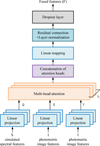 |
Fig. 9 Workflow of the multi-head attention module. |
3.5 Model training
As described in Sect. 2, we obtained a total of 36278 imagespectrum pairs. Before training our MMLforGalAM, the dataset is divided into training, validation, and test sets in an 8:1:1 ratio. During training, the model uses the training set to minimise the loss function, enabling it to learn effectively and make accurate predictions. The validation set monitors the performance during training, prevents overfitting, and guides the hyperparameter tuning. The test set provides an evaluation of predictive performance on unseen data. Figure 10 shows the distributions of age and metallicity in the training, validation, and test sets. It demonstrates the consistency of these parameter distributions across the three subsets.
In the training process of MMLforGalAM, all models use the mean squared error (MSE) as the loss function, defined in Eq. (8). MSE calculates the average square difference between predicted values ( ) and true values (
 ). In addition, the adaptive moment estimation (Adam) optimizer is applied for learning. We performed a grid search over three learning rates (0.001, 0.0001, and 0.00001) for the models. After comparative experiments to optimize model performance, ℳ1, ℳ3, and ℳ4 were set to a learning rate of 0.0001, while ℳ2 employed a learning rate of 0.001. The MSE calculation is:
 (8)
(8)
Each model in the framework of our MMLforGalAM is trained for 100 epochs to ensure sufficient optimization. Through the iterative training process, each model gradually optimizes its parameters, resulting in improved predictive performance for galaxy parameters. The training and validation loss curves shown in Fig. 11 indicate that the loss values stabilized around 80−100 epochs, with a steady decrease observed in both training and validation losses. The minimal gap between these losses indicates that the final model exhibits good generalisation capabilities.
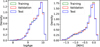 |
Fig. 10 Distributions of age and metallicity in the training, validation, and test sets. The x-axis represents the parameter value ranges, and the y-axis indicates the sample density within each interval. |
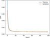 |
Fig. 11 Loss curves of MMLforGalAM for the training set and validation set across epochs. |
4 Experiments
The experiments were conducted on a server equipped with an NVIDIA GeForce RTX 3080 Ti GPU with 12 GB of memory and an Intel 11th Gen Core i7-11700F CPU. The system runs on Linux and the model training is conducted with the Keras library (Chollet & others 2018). The software environment includes Python 3.8.5, TensorFlow-GPU 2.10.0, NumPy 1.24.4, Matplotlib 3.7.2, and Scikit-learn 1.3.0.
To assess the computational efficiency of our model, we measured both the training and inference times used by our model. Specifically, training our model on our training set of approximately 29000 samples takes 2 hours. For the inference time evaluation, we used our test set of approximately 3600 images and fed them into the trained model. On average, predicting the age and metallicity for each image takes 1.5 seconds. For future large-scale astronomical surveys, if the observational properties (including image resolution and filter systems) are similar to those of SDSS, our trained MMLforGalAM model can be directly used to infer the age and metallicity. Given the model’s 1.5 -second per-image prediction speed on a single GPU such as ours, processing a large dataset such as 1 million images would take approximately 17 days. However, if the observational properties differ significantly, retraining our MMLforGalAM model would be necessary. In this case, training on significantly larger datasets would require more powerful GPUs, multi-GPU training, or distributed computing frameworks to ensure feasible training times.
4.1 Evaluation metrics
To evaluate and compare the performance of MMLforGalAM, several metrics are utilised: mean squared error (MSE), mean absolute error (MAE), bias, and standard deviation (SD).
The MSE is defined as shown in Eq. (8). MAE (Eq. (9)) calculates the average absolute difference between predictions and true values, offering a straightforward measure of prediction error. Bias, defined in Eq. (10), quantifies systematic error by measuring the average difference between predicted and true values, indicating whether the model consistently overestimates or underestimates. SD (Eq. (11)) reflects the variability of the predictions, serving as an essential metric for assessing the consistency and robustness of the model. The mathematical definitions of these metrics are as follows:
 (9)
(9)
 (10)
(10)
 (11)
(11)
where  represents the predicted value of the i-th sample,
  is the true value of the i-th sample, and n is the total number of samples. By analysing these metrics, we can gain a detailed understanding of the model’s predictive performance and accuracy.
4.2 Model evaluation
To evaluate the performance of the multi-modal learning model (MMLforGalAM) in predicting galaxy age and metallicity, we designed four sets of experiments. In Sect. 4.2.1, we analyse the differences between the predicted values obtained from MMLforGalAM and the true values. Section 4.2.2 compares the simulated spectral features generated by the spectral generation model ℳ2 with real spectral features to validate the reliability of ℳ2. In Sect. 4.2.3, we compare the performance of our multimodal model with an image-only model, which relies solely on photometric images. Finally, Sect. 4.2.4 examines the performance of the multi-modal model against a spectra-only model, which relies only on spectra.
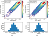 |
Fig. 12 Comparison of age in log (yr) and metallicity ([M/H]) between the predicted values from our MMLforGalAM and true values: panel (a) shows the comparison for age and panel (b) shows the results of metallicity. In the bottom panels, Δlog Age represents the difference between the predicted and true values of age, while Δ[M/H] represents the difference of metallicity. Note: the points out of 3σ are clipped. |
4.2.1 Comparison of predictions using our MMLforGalAM and true ones
To visualise the differences between the predicted values generated by our method MMLforGalAM and true ones, we plot the results in Fig. 12. Panel (a) illustrates the comparison for age, while panel (b) shows the comparison for metallicity. In both of the top panels, most data points lie close to the red dashed line, indicating minimal bias in the predictions. In addition, the bottom panels display the residuals (ypred − ytrue) concentrated around zero, suggesting low bias in the model’s predictions. The top-left corner of each figure shows the bias and SD for the differences between predicted and true values. For age, the bias is 0.0034 dex, and the SD is 0.1506 dex. For metallicity, the bias is -0.0091 dex and the SD is 0.1402 dex. The low bias and SD for both age and metallicity demonstrate the reliability and accuracy of our multi-modal model.
4.2.2 Comparison of simulated spectral features from model ℳ2 and real spectral features
The model ℳ2 is designed to generate simulated spectral features from photometric images, capturing information related to galaxy age and metallicity. To assess the effectiveness of the spectral feature generation model, ℳ2, we compared the simulated spectral features to the corresponding true spectral features from observed galaxy spectra.
Figure 13 displays an example of simulated spectral features alongside their real ones. The upper panel illustrates the spectral features (normalising to [0,1]) with the red and blue curves representing the simulated and true spectral features, respectively. The lower panel shows the residuals between the simulated and true spectral features. From the residuals, we find that they generally fall within the range of [−0.05,0.05]. This result visually validates that ℳ2 effectively captures the underlying spectral characteristics from photometric images.
Furthermore, we quantified the agreement between our generated spectra and real spectra using the R-squared ( R2 ) metric. Specifically, R2 was calculated as  , where SSres is the sum of squares of residuals (ypred − ytrue ytrue − mean (ytrue)). This metric measures the proportion of variance in a real spectrum that is explained by its generated spectrum, ranging from 0 to 1, where values closer to 1 indicate a better fit. Figure 13 shows R2 = 0.9981 for a specific example. In addition, using all images in the test set, we compared the simulated and true spectral features and computed their R2, yielding an average R2 of 0.9767. This result quantitatively confirms the effectiveness of ℳ2 in generating reliable spectral features.
To further evaluate the direct impact of ℳ2 on prediction performance, we conducted an ablation study by training MMLforGalAM without ℳ2. Specifically, we removed ℳ2 from the MMLforGalAM framework, directly feeding the real spectral features extracted by ℳ1 into the ℳ4. The modified model(hereafter, MMLforGalAMwithReal) is trained and tested using the same datasets as the MMLforGalAM, achieving bias and SD values of -0.0088 and 0.1293 dex for the age, and -0.0175 and 0.1266 dex for the metallicity, detailed in Table 1. Compared to these results, our MMLforGalAM with ℳ2, which achieves an SD of 0.1506 dex for age and 0.1402 dex for metallicity, performs only slightly lower than it would when we are using real spectral features. The results suggest that ℳ2 can capture spectral information and contribute to the overall prediction accuracy of MMLforGalAM.
 |
Fig. 13 Example of spectral features generated by model ℳ2 and true spectral features extracted from observed galaxy spectra. The upper panel shows the normalised spectral features ([0,1]), with red and blue curves representing the simulated and true features, respectively. The lower panel shows the residuals between the simulated and true spectral features. |
4.2.3 Comparison of the multi-modal model and the image-only model
This section compares the performance of our MMLforGalAM with a single-modal model based solely on photometric images (hereafter referred to as the image-only model). The architecture of the image-only model is identical to that of the ℳ3 in MMLforGalAM (see Fig. 7). To ensure a fair comparison, we kept the key hyperparameters − including the loss function, learning rate, optimiser settings, and training epochs - consistent between the two models. This image-only model was trained and tested using the same datasets as the MMLforGalAM. The prediction results of the image-only model are shown in Fig. 14. For age predictions by the image-only model, the bias and SD are 0.0426 and 0.2057 dex, respectively; whereas for the metallicity predictions, they are 0.0122 and 0.1644 dex.
Table 1 summarises the evaluation metrics (detailed in Sect. 4.1) for MMLforGalAM and other single-modal models. As shown in Table 1, all metrics for MMLforGalAM are lower than those for the image-only model.
The MSE (see Eq. (8)) of our MMLforGalAM is 0.0227 and 0.0197 for age and metallicity, respectively. In comparison, the corresponding MSE values for the image-only model are 0.0441 and 0.0272.
In terms of the MAE, defined in Eq. (9), our model also performs better, with values of 0.1215 for age and 0.1121 for metallicity, compared to 0.1684 and 0.1302 for the imageonly model.
The SD (see Eq. (11)) for the age is 0.1506 for our model, compared to 0.2057 for the image-only model, representing a 27% reduction. Similarly, for metallicity, our model achieves an SD of 0.1402, which is 15% lower than the 0.1644 observed for the image-only model.
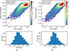 |
Fig. 14 Prediction results for age in log (yr) and metallicity ([M/H]) using the image-only model, which is based only on images: (a) shows the comparison for age and (b) shows the comparison for metallicity. |
4.2.4 Comparison of the multi-modal model and the spectra-only model
In this section, we compare the performance of MMLforGalAM with a single-modal model based solely on spectra (hereafter spectra-only model). The spectra-only model shares the same architecture as ℳ1 (illustrated in Fig. 5). All hyperparameters including the loss function, learning rate, optimiser settings, and training epochs are consistent between the two models.
The spectra-only model was trained and tested using the same datasets as the MMLforGalAM. Figure 15 illustrates the performance of this model. The SDs of its age and metallicity predictions are 0.1355 dex and 0.1269 dex, respectively. This performance is slightly better than MMLforGalAM’s performance ( 0.1506 dex for age and 0.1402 dex for metallicity). Other metrics are given in Table 1. This performance difference may be attributed to the fact that MMLforGalAM relies on simulated spectral features generated by ℳ2, instead of directly utilising real spectra. As demonstrated by the ablation study (described in Sect. 4.2.2), MMLforGalAM relies on simulated spectral features and performs slightly lower than when using real spectral features (MMLforGalAMwithReal).
However, it is crucial to remember that the primary goal of MMLforGalAM is to provide estimates in the absence of spectra. MMLforGalAM is designed to work when we only have images without spectra, which is a scenario where the spectraonly model cannot function. In this work, we provide two trained models to predict the age and metallicity: the spectra-only model and the MMLforGalAM model. If spectra of galaxies are available, we recommend using our trained spectra-only model to obtain more precise age and metallicity estimates. If only images are available, MMLforGalAM offers a robust and effective solution, and we recommend its use. We note that we have not provided the MMLforGalAMwithReal model here. Although the MMLforGalAMwithReal model offers only a slight gain in accuracy compared to the spectra-only model (comparison in Table 1), it requires more extensive image pre-processing. Therefore, we believe the spectra-only model represents a more practical and efficient solution when spectra are available.
Comparison of age and metallicity prediction among different models.
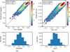 |
Fig. 15 Prediction results for age in log (yr) and metallicity ([M/H]) using the spectra-only model, which is based only on spectra: (a) shows the comparison for age and (b) shows the comparison for metallicity. |
4.3 Model applicability at different signal-to-noise ratios
This section is aimed at exploring the performance of the MMLforGalAM model at different S/Ns. Specifically, we divided the test set into six S/N intervals: [5, 10), [10, 15), [15, 20), [20, 25), [25,30), and [30,∞). We predicted the age and metallicity of galaxies in each subset by our well-trained model. The scatters of the model predictions in each S/N range are shown as black solid lines in Fig. 16. The upper panel of this figure illustrates the variation in the standard deviation of age with S/N, while the lower panel presents the corresponding trend for metallicity. As shown by the black solid line in Fig. 16, the scatters of the model predictions generally decrease as S/N increases. Even in the low S/N interval ( 5≤S/N<10 ), where noise levels are relatively high, the model still maintains reasonable accuracy, achieving a scatter of approximately 0.18 dex at S/N=5. This indicates that the model provides useful estimates even for lower quality spectra.
In addition, we also quantitatively assessed the intrinsic uncertainty of the pPXF-derived parameters using a Monte Carlo perturbation analysis. Specifically, for each spectrum in our test set, we applied Gaussian noise to generate 100 noisy realizations. The level of noise added is consistent with the flux errors in the original spectrum. Each spectrum F(λ) was perturbed by adding Gaussian noise as shown in Eq. (12):
 (12)
(12)
where  follows a Gaussian perturbation N(μ,σ2) with μ = 0 and σ2 determined from the flux errors of the original spectrum.
We then apply pPXF to these 100 perturbed spectra to derive the corresponding age and metallicity values. The standard deviation of these 100 measurements is taken as the intrinsic dispersion of pPXF-derived age and metallicity of the spectrum, F(λ). The intrinsic dispersions of pPXF-derived parameters at different S/N bins in our test set are shown as black dotted lines in Fig. 16. We can see that the intrinsic dispersions in both age and metallicity generally decrease with increasing S/N. With the exception of the S/N = 5, where the intrinsic dispersion is slightly larger (below 0.07 dex), the dispersion remains below 0.05 dex across all S/N bins. In addition, we also see that the model’s prediction error (as shown by the solid black lines in Fig. 16) tends to converge toward the intrinsic dispersion (dashed black lines) at higher S/N values. This suggests that the higher S/N of spectra, the closer the predicted value of the model is to the given label. In conclusion, we believe that the uncertainties in the pPXF-derived labels, while present, do not significantly hinder the model’s ability to learn the underlying relationships between spectral features and galaxy properties.
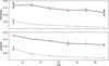 |
Fig. 16 The scatters of model prediction and intrinsic uncertainties of pPXF-derived parameters across different ranges of S/N. The black solid lines represent the standard deviation of the difference between predicted values and true ones in different S/N subsets. The black dotted lines display the intrinsic dispersions of the pPXF-derived parameters measured by a Monte Carlo perturbation analysis. |
5 Summary
This study presents a multi-modal regression method for estimating the age and metallicity of galaxies. The key contributions and innovations of this research are as follows: first, we extracted knowledge of the real spectra (model ℳ1) and then converted photometric images to spectral features (model ℳ2). Using the simulated spectral feature generator, ℳ2, our approach, which minimises the reliance on spectroscopic data, offers advantages when spectra are incomplete or absent. Second, we proposed a multi-modal data fusion strategy (model ℳ4) utilising a multihead attention mechanism to effectively integrate the spectral features from model ℳ2 with image features from model ℳ3. This mechanism captures complex relationships between image and spectral features, enhances feature selection, and improves the prediction accuracy by focussing on the most relevant information from both modalities.
These experimental results demonstrate that our multi-modal model achieves higher prediction accuracy for age and metallicity, compared to the single-modal model based solely on images. Specifically, the SD for age prediction using the multi-modal model is 0.1506 dex and for the metallicity prediction, it is 0.1402 dex. Compared to the single-modal model, these SDs represent reductions of 27% and 15% for the age and metallicity, respectively.
Future works will be focussed on extending the multi-modal approach to predict other galaxy properties, such as stellar mass and star formation rates. Furthermore, we aim to refine the attention mechanism to better adapt them to large-scale astronomical surveys, ensuring scalability and robustness for diverse observational conditions.
Data availability
The two trained models (spectra-only model and MMLfor-GalAM model) and related code are publicly available at https://github.com/liping523/MMLforGalAM
Acknowledgments
This work was supported by the Natural Science Foundation of China (grant Nos. 12273075, 11903008, and U1931106), Dezhou University (grant no. HXKT2023006). Yan-Ke Tang is supported by the International Centre of Supernovae, Yunnan Key Laboratory (nos. 202302AN360001 and 202302AN36000103).
References
- Bonjean, V., Aghanim, N., Salomé, P., et al. 2019, A&A, 622, A137 [NASA ADS] [CrossRef] [EDP Sciences] [Google Scholar]
- Brinchmann, J., Charlot, S., White, S. D. M., et al. 2004, MNRAS, 351, 1151 [Google Scholar]
- Bruzual, G., & Charlot, S. 2003, MNRAS, 344, 1000 [NASA ADS] [CrossRef] [Google Scholar]
- Cappellari, M. 2017, MNRAS, 466, 798 [Google Scholar]
- Cappellari, M. 2023, MNRAS, 526, 3273 [NASA ADS] [CrossRef] [Google Scholar]
- Cappellari, M., & Emsellem, E. 2004, PASP, 116, 138 [Google Scholar]
- Chevallard, J., & Charlot, S. 2016, MNRAS, 462, 1415 [NASA ADS] [CrossRef] [Google Scholar]
- Chollet, F., & others. 2018, Keras: The Python Deep Learning library, Astrophysics Source Code Library [record ascl:1806.022] [Google Scholar]
- Cid Fernandes, R., Mateus, A., Sodré, L., Stasińska, G., & Gomes, J. M. 2005, MNRAS, 358, 363 [Google Scholar]
- Cui, X.-Q., Zhao, Y.-H., Chu, Y.-Q., et al. 2012, Res. Astron. Astrophys., 12, 1197 [Google Scholar]
- Dey, A., Schlegel, D. J., Lang, D., et al. 2019, AJ, 157, 168 [Google Scholar]
- Euclid Collaboration (Mellier, Y., et al.) 2025, A&A, 697, A1 [Google Scholar]
- Gai, M., Bove, M., Bonetta, G., Zago, D., & Cancelliere, R. 2024, MNRAS, 532, 1391 [Google Scholar]
- Gallazzi, A., Charlot, S., Brinchmann, J., White, S. D. M., & Tremonti, C. A. 2005, MNRAS, 362, 41 [Google Scholar]
- Gallazzi, A., Charlot, S., Brinchmann, J., & White, S. D. M. 2006, MNRAS, 370, 1106 [Google Scholar]
- Gomes, J. M., & Papaderos, P. 2017, A&A, 603, A63 [NASA ADS] [CrossRef] [EDP Sciences] [Google Scholar]
- Henghes, B., Thiyagalingam, J., Pettitt, C., Hey, T., & Lahav, O. 2022, MNRAS, 512, 1696 [NASA ADS] [CrossRef] [Google Scholar]
- Hong, S., Zou, Z., Luo, A. L., et al. 2023, MNRAS, 518, 5049 [Google Scholar]
- Hoyle, B. 2016, Astron. Comput., 16, 34 [NASA ADS] [CrossRef] [Google Scholar]
- Kennicutt, Jr., R. C. 1998, ARA&A, 36, 189 [Google Scholar]
- Laureijs, R., Amiaux, J., Arduini, S., et al. 2011, arXiv e-prints [arXiv:1110.3193] [Google Scholar]
- Liew-Cain, C. L., Kawata, D., Sánchez-Blázquez, P., Ferreras, I., & Symeonidis, M. 2021, MNRAS, 502, 1355 [NASA ADS] [CrossRef] [Google Scholar]
- LSST Science Collaboration (Abell, P. A., et al.) 2009, arXiv e-prints [arXiv:0912.0201] [Google Scholar]
- LSST Dark Energy Science Collaboration 2012, arXiv e-prints [arXiv:1211.0310] [Google Scholar]
- Luo, A.-L., Zhao, Y.-H., Zhao, G., et al. 2015, Res. Astron. Astrophys., 15, 1095 [Google Scholar]
- Maraston, C. 2005, MNRAS, 362, 799 [NASA ADS] [CrossRef] [Google Scholar]
- Maraston, C., & Strömbäck, G. 2011, MNRAS, 418, 2785 [Google Scholar]
- Ocvirk, P., Pichon, C., Lançon, A., & Thiébaut, E. 2006, MNRAS, 365, 46 [Google Scholar]
- Parker, L., Lanusse, F., Golkar, S., et al. 2024, MNRAS, 531, 4990 [Google Scholar]
- Petrosian, V. 1976, ApJ, 210, L53 [NASA ADS] [CrossRef] [Google Scholar]
- Surana, S., Wadadekar, Y., Bait, O., & Bhosale, H. 2020, MNRAS, 493, 4808 [NASA ADS] [CrossRef] [Google Scholar]
- Tojeiro, R., Heavens, A. F., Jimenez, R., & Panter, B. 2007, MNRAS, 381, 1252 [NASA ADS] [CrossRef] [Google Scholar]
- Vaswani, A. 2017, Advances in Neural Information Processing Systems [Google Scholar]
- Vazdekis, A., Sánchez-Blázquez, P., Falcón-Barroso, J., et al. 2010, MNRAS, 404, 1639 [NASA ADS] [Google Scholar]
- Vazdekis, A., Koleva, M., Ricciardelli, E., Röck, B., & Falcón-Barroso, J. 2016, MNRAS, 463, 3409 [Google Scholar]
- Wang, L.-L., Shen, S.-Y., Luo, A. L., et al. 2022, ApJS, 258, 9 [Google Scholar]
- Wang, L.-L., Yang, G.-J., Zhang, J.-L., et al. 2024, MNRAS, 527, 10557 [Google Scholar]
- Wilkinson, D. M., Maraston, C., Thomas, D., et al. 2015, MNRAS, 449, 328 [NASA ADS] [CrossRef] [Google Scholar]
- Wilkinson, D. M., Maraston, C., Goddard, D., Thomas, D., & Parikh, T. 2017, MNRAS, 472, 4297 [Google Scholar]
- Wu, J. F., & Boada, S. 2019, MNRAS, 484, 4683 [NASA ADS] [CrossRef] [Google Scholar]
- Wu, Y., Tao, Y., Fan, D., Cui, C., & Zhang, Y. 2024, MNRAS, 527, 1163 [Google Scholar]
- York, D. G., Adelman, J., Anderson, John E. J., et al. 2000, AJ, 120, 1579 [NASA ADS] [CrossRef] [Google Scholar]
- Zeraatgari, F. Z., Hafezianzadeh, F., Zhang, Y. X., Mosallanezhad, A., & Zhang, J. Y. 2024, A&A, 688, A33 [NASA ADS] [CrossRef] [EDP Sciences] [Google Scholar]
- Zhong, J., Deng, Z., Li, X., et al. 2024, MNRAS, 531, 2011 [CrossRef] [Google Scholar]
Appendix A Effects of resolutions and filters of SDSS photometric images on model performance
To determine the optimal image resolution and filter combination of photometric images for our deep learning model, we designed two comparative experiments to investigate how image resolutions and filters affect the prediction of age and metallicity.
(1) Image resolutions:
We compared the effects of two different resolutions, 64×64 and 128×128, on model performance. While we plan to evaluate 256×256 resolution, we are unfortunately limited by system resource constraints (memory and GPU capacity).
The experimental procedure is as follows: We download the images at 64×64 and 128×128 resolutions. Using the same image pre-processing methods described in Sect. 2.2, we pre-process the images for both resolutions. We then train and evaluate two models, one for each resolution, using the model architecture and hyperparameter settings described in Sect. 3. The evaluation metrics for model predictions at each resolution are presented in Table A.1.
Comparison of age and metallicity prediction for our MMLforGalAM using different image resolutions.
The results indicate that the MMLforGalAM model trained with 128 × 128 resolution images outperforms the model trained with 64 × 64 resolution images, exhibiting lower standard deviations ( 0.1483 vs .0 .1968 for age and 0.1290 vs .0 .1697 for metallicity). This improvement is primarily attributed to the ability of higher resolution images to capture finer details and more subtle features of the galaxies.
(2) Image filter bands:
In Sect. 2.1.2, we describe that our downloaded SDSS images are three-colour JPEG images which are generated by converting the g, r, and i bands into a three-colour composite (i − r − g to R-G-B) obtained from the SDSS ImgCutout service. To assess the influence of individual bands and combinations of two bands on model performance, we conduct experiments using the following inputs: individual g, r, and i bands, as well as combinations of two bands (gr,gi, and ri ). Table A. 2 shows the various metrics of MMLforGalAM’s predictions of age and metallicity under different bands. The results clearly demonstrate that the gri-band combination yields the best performance, exhibiting the lowest MSE, MAE, and standard deviation in both predictions. This is because more colour information, derived from the combination of g, r, and i bands, captures spectral features on the surface of galaxies, providing valuable constraints on galaxy properties.
Comparison of age and metallicity prediction for our MMLforGalAM using different filter bands as input.
We retrieve BPT classifications from SDSS MPA-JHU catalogue (Brinchmann et al. 2004) for galaxy spectra in SDSS DR7. It reveals that 95.5% of excluded spectra (z>0.3) are unclassifiable (bptclass=-1), often representing unclassifiable galaxies with weak or absent emission lines. However, in our selected dataset after applying our redshift cut, galaxies with bptclass = −1 still constitute approximately 37%. Therefore, it suggests that our redshift cut does not severely limit the diversity of galaxy types in our sample.
All Tables
Comparison of age and metallicity prediction for our MMLforGalAM using different image resolutions.
Comparison of age and metallicity prediction for our MMLforGalAM using different filter bands as input.
All Figures
|
Fig. 1 Comparison of the redshift, S/N, and magnitude (petroMag_r) distributions between the randomly selected sample and the full dataset. |
| In the text | |
|
Fig. 2 Examples of photometric images and their corresponding spectra with different S/Ns. In each panel, the right ascension (RA) and declination (Dec), redshift, and S/N of the galaxy are given on the upper-right corner. |
| In the text | |
|
Fig. 3 Workflow of photometric image pre-processing: (a) shows the original images of blended and unblended galaxies; (b) displays the images after masking noisy sources; (c) presents the unblended image after identification and cropping; (d) shows the blended image, which has been discarded. |
| In the text | |
|
Fig. 4 Framework of the MMLforGalAM. |
| In the text | |
|
Fig. 5 Architecture of the spectral feature extraction model (ℳ1). The shape of each layer is represented as a × b × c or a × b, where a × b represents the feature map dimensions and c is the number of convolutional filters. The red dashed box represents the final fully connected layer, whose output serves as the label for training the next model, ℳ2. |
| In the text | |
|
Fig. 6 Architecture of the simulated spectral feature generation model (ℳ2). The numbers in the form a × b × c or a × b for each layer are consistent with Fig. 5. |
| In the text | |
|
Fig. 7 Architecture of the image feature extraction model (ℳ3). The red dashed box highlights the image features related to age and metallicity, which are used as input to the multi-modal model (ℳ4). |
| In the text | |
|
Fig. 8 Architecture of the multi-modal attention regression model (ℳ4). |
| In the text | |
|
Fig. 9 Workflow of the multi-head attention module. |
| In the text | |
|
Fig. 10 Distributions of age and metallicity in the training, validation, and test sets. The x-axis represents the parameter value ranges, and the y-axis indicates the sample density within each interval. |
| In the text | |
|
Fig. 11 Loss curves of MMLforGalAM for the training set and validation set across epochs. |
| In the text | |
|
Fig. 12 Comparison of age in log (yr) and metallicity ([M/H]) between the predicted values from our MMLforGalAM and true values: panel (a) shows the comparison for age and panel (b) shows the results of metallicity. In the bottom panels, Δlog Age represents the difference between the predicted and true values of age, while Δ[M/H] represents the difference of metallicity. Note: the points out of 3σ are clipped. |
| In the text | |
|
Fig. 13 Example of spectral features generated by model ℳ2 and true spectral features extracted from observed galaxy spectra. The upper panel shows the normalised spectral features ([0,1]), with red and blue curves representing the simulated and true features, respectively. The lower panel shows the residuals between the simulated and true spectral features. |
| In the text | |
|
Fig. 14 Prediction results for age in log (yr) and metallicity ([M/H]) using the image-only model, which is based only on images: (a) shows the comparison for age and (b) shows the comparison for metallicity. |
| In the text | |
|
Fig. 15 Prediction results for age in log (yr) and metallicity ([M/H]) using the spectra-only model, which is based only on spectra: (a) shows the comparison for age and (b) shows the comparison for metallicity. |
| In the text | |
|
Fig. 16 The scatters of model prediction and intrinsic uncertainties of pPXF-derived parameters across different ranges of S/N. The black solid lines represent the standard deviation of the difference between predicted values and true ones in different S/N subsets. The black dotted lines display the intrinsic dispersions of the pPXF-derived parameters measured by a Monte Carlo perturbation analysis. |
| In the text | |
Current usage metrics show cumulative count of Article Views (full-text article views including HTML views, PDF and ePub downloads, according to the available data) and Abstracts Views on Vision4Press platform.
Data correspond to usage on the plateform after 2015. The current usage metrics is available 48-96 hours after online publication and is updated daily on week days.
Initial download of the metrics may take a while.