| Issue |
A&A
Volume 698, June 2025
|
|
|---|---|---|
| Article Number | A239 | |
| Number of page(s) | 27 | |
| Section | Astrophysical processes | |
| DOI | https://doi.org/10.1051/0004-6361/202453499 | |
| Published online | 17 June 2025 | |
A census of galactic spider binary millisecond pulsars with the Nançay Radio Telescope
1
LPC2E, OSUC, Univ Orléans, CNRS, CNES, Observatoire de Paris, F-45071 Orléans, France
2
Observatoire Radioastronomique de Nançay, Observatoire de Paris, Université PSL, Université d’Orléans, CNRS, 18330 Nançay, France
3
LUX, Observatoire de Paris, Université PSL, Sorbonne Université, CNRS, 92190 Meudon, France
⋆ Corresponding author: This email address is being protected from spambots. You need JavaScript enabled to view it.
Received:
18
December
2024
Accepted:
12
April
2025
Abstract
Context. Spider binary pulsars are systems in which a millisecond pulsar (MSP) tightly orbits (Pb ≲ 1 day) a low mass (mc ≲ 0.5 M⊙) non-degenerate or semi-degenerate star. Spider systems often display eclipses around superior conjunction, and their orbital periods often exhibit rapid time variations. The eclipse phenomenon is currently poorly understood. However, eclipses are excellent probes of plasma physics and intrabinary shocks, and they can also be used to study MSP formation processes.
Aims. In this work, we present Nançay Radio Telescope (NRT) observations of a sample of 19 spider pulsars conducted over several years. The sample includes 11 eclipsing and eight non-eclipsing systems. We aim to provide a homogeneous phenomenological study of the eclipses in order to compare spiders and study their group properties, as those eclipsing systems are often studied individually. We compare our results with those derived from other studies, mainly optical observations and analyses of the pulsar companions.
Methods. We analysed eclipses via pulsar timing by using a 2D template-matching technique that allowed us to simultaneously determine radio pulse times of arrival (TOAs) and dispersion measures (DMs) along the lines of sight to the pulsars. The eclipses were then fit with a phenomenological model that gives a measurement of the duration and asymmetry of the eclipses. We then compared these parameters to other eclipse and system measurements in order to discuss the potential link between the presence of eclipses and orbital inclination, as eclipsing systems are known to have higher mass functions than non-eclipsing ones. Finally, we formed polarisation-calibrated profiles for the pulsars in our sample and derived some of their main polarisation properties.
Results. We present a comprehensive review of the NRT NUPPI backend spider pulsar dataset. We also present the first review and systematic analysis of a large sample of eclipsers monitored with the NRT over several years. The phenomenological fit allowed us to derive a number of parameters to compare the eclipsers with each other, which led to the categorisation of eclipsers depending on the shape of their eclipses. We present the polarimetric properties of the 19 spiders in the sample alongside their profiles, which were previously unpublished in some cases. We compared the mass function distributions of the eclipsing and non-eclipsing systems in our sample and found (in agreement with previous studies) that eclipsing systems have higher mass functions than their non-eclipsing counterparts, suggesting that the latter have lower orbital inclinations. For the eclipsing systems, we found evidence of a positive correlation between eclipse duration and mass function, as expected if more eclipsing material crosses the line of sight in higher inclination systems. For the entire sample, we found marginal evidence for increasing pulse profile width with decreasing mass function, possibly indicating that the low mass function spiders are indeed those seen under low inclinations. Finally, we conducted a comprehensive literature review of the published inclination measurements for the pulsars in the sample and compared the inclinations to eclipse parameters, (unexpectedly) finding no clear correlations between orbital inclination and eclipse properties. Nevertheless, the small number of available orbital inclination constraints, which contradict each other in some cases, hinders such searches for correlations.
Key words: binaries: eclipsing / pulsars: general
© The Authors 2025
 Open Access article, published by EDP Sciences, under the terms of the Creative Commons Attribution License (https://creativecommons.org/licenses/by/4.0), which permits unrestricted use, distribution, and reproduction in any medium, provided the original work is properly cited.
This article is published in open access under the Subscribe to Open model. This email address is being protected from spambots. You need JavaScript enabled to view it. to support open access publication.
1. Introduction
Since the discovery of the first spider pulsar B1957+20, the so-called original black widow (BW) pulsar (Fruchter et al. 1988), these extreme binary systems have been used to study a broad range of physics. Spider binaries are usually defined as millisecond pulsars (MSPs) in tight orbits (Pb ≲ 1 day) with light and non-degenerate or semi-degenerate stars. Depending on the companion mass, the spiders are divided into two sub-populations: BWs, which have the lightest companions (mc ≲ 0.07 M⊙), and redbacks (RBs), which have sub-solar companions (0.07 M⊙ ≲ mc ≲ 0.5 M⊙) (Roberts 2013). In these systems, the powerful pulsar winds ablate the outer layers of the tidally locked companion. Neutron stars (NSs) are the cornerstone of several research fields, such as general relativity tests, astronomical transients studies, gravitational wave astronomy, and investigations of the equation of state (EoS). Different EoSs allow for different mass-radius relationships and different maximum masses. Therefore, measuring as many NS masses as possible is key to constraining EoSs. The MSPs have an average mass higher than that of young pulsars (Özel & Freire 2016), and spiders are believed to have high masses among MSPs (Linares 2020). However, as noted in Clark et al. (2023), the mass measurements for spider pulsars, which are often obtained from optical observations, may be overestimated because of the underestimated inclinations coming from oversimplified heating models, especially in the case of BWs. Recent measurements from the same team have brought back some spider masses closer to the average mass value for MSPs.
The MSPs are rotation-powered NSs with short rotational periods (P ≲ 10 ms) that are believed to have been spun up by accretion and thus by the transfer of angular momentum from a binary companion (Bisnovatyi-Kogan & Komberg 1974; Alpar et al. 1982). Spiders are thought to be a possible evolutionary channel for isolated MSPs (Ruderman et al. 1989). The binary stage would therefore be a temporary phase during which the pulsar accretes and ablates its companion. During this phase, the rotation of the pulsar is spun up via the transfer of angular momentum. This idea is supported by the transitioning systems that have been seen to switch back and forth from an accretion state (X-ray emitting, radio-quiet) to an RB state during the past two decades (see e.g. Papitto et al. 2013; Bassa et al. 2014; Roy et al. 2015).
Spiders often undergo “eclipses” around superior conjunction during a fraction of the orbital period. It is not the companion that occults the beam but the matter around it, which corresponds to the ablated material outflowing from the companion. This fog is not gravitationally bound to the companion, as it is very often larger than its Roche lobe. The exact physical mechanism is currently unclear, but the eclipses are usually explained by dispersion, scattering, and absorption of radio emission by the diffuse intrabinary material. A review of the different eclipse mechanisms can be found in Thompson et al. (1994). Some works have linked individual systems to specific mechanisms. For instance, scattering and cyclotron absorption are considered the primary mechanisms producing the eclipses of PSR J2051−0827, while for PSR J1544+4937, cyclotron-synchrotron absorption is believed to be the dominant eclipse mechanism at play (Kansabanik et al. 2021). We note that their study used observations conducted around 400 MHz, where PSR J1544+4937 displays eclipses, but this pulsar does not display eclipses at 1.4 GHz. Most of the processes at stake depend on the observation frequency, so eclipse properties also depend on frequency, and studying these phenomena at different radio frequencies is thus important. As dispersive effects are strongest at low frequencies, eclipses of spider systems have often been observed and studied below ∼1 GHz. Studies of eclipse properties of pulsars at frequencies above 1 GHz have been conducted (see e.g. Polzin et al. 2019); however, to our knowledge, no systematic studies of the properties of ensembles of eclipsing pulsars have been published at these high frequencies.
The Nançay Radio Telescope (NRT) is a meridian telescope equivalent to a 94 m parabolic dish, and it is located near Orléans, France. The NRT can track objects with declinations above ∼ − 39° for approximately 1 h around transit. Detailed descriptions of the telescope and of pulsar observations with the NRT can be found in Guillemot et al. (2023). The NRT has been observing spiders for more than two decades, monitoring known systems and searching for new ones. Notably, one BW has been discovered with NRT, PSR J2055+3829 (Guillemot et al. 2019), which was found during the SPAN512 survey (Desvignes et al. 2013, 2022). This paper constitutes the first effort to systematically analyse the L-band data on the sample of spider systems observed with the NRT. Thus, it provides an opportunity to look into their group properties.
We present the analysis of NRT data on 19 spiders observed over several years. In Sect. 2, we describe the sources included in this census, and their properties derived from timing and optical observations. In Sect. 3, we present the analysis conducted for this work: the data preparation and timing method (Sect. 3.1), the eclipse characterisation (Sect. 3.2), and the morphological analysis of their eclipses (for pulsars exhibiting eclipses; see Sect. 3.3). Section 4 presents an overview of their polarimetric properties. Results are presented in Sect. 5, including the correlations between the eclipse parameters (Sect. 5.1) and the dependence of eclipse parameters on the mass function (Sect. 5.2) as well as on orbital inclination (Sect. 5.3). Section 5.4 presents a search for correlation between pulse profile widths and the mass functions of the systems. Finally, we summarise our work in Sect. 6.
2. Pulsar sample and dataset properties
Since the beginning of pulsar monitoring programs at Nançay, a total of 19 spider pulsars have been followed regularly with the NRT. Before mid-2011, pulsars were observed with the Berkeley-Orléans-Nançay (BON) backend, and in August 2011 BON was replaced by the NUPPI backend as the primary pulsar instrumentation in operation at Nançay. The NUPPI pulsar observation backend is a version of the Green Bank Ultimate Pulsar Processing Instrument1 designed for Nançay. It records 512 MHz of frequency bandwidth, in the form of 128 channels of 4 MHz each, that are coherently dedispersed in real time. In this article we only considered data taken with the NUPPI backend, since NUPPI observations of spider pulsars are much more numerous and of higher quality than BON observations. The majority of NUPPI observations have been conducted at L-band, at a central frequency of 1484 MHz.
Figure 1 puts the pulsar sample into the context of the known spider pulsar population as listed in the ATNF catalogue (Manchester et al. 2005)2. The names of the 19 spider pulsars in our sample, as well as an overview of the NRT dataset considered in this study for these pulsars can be seen in Fig. 2. In Table 1 we list the total time spans of the observations and the number of observations for each pulsar. We note that there is only one RB pulsar in our sample: PSR J1628−3205. All the other objects are BW pulsars. In spite of the under-representation of RB-type objects in our sample, orbital periods and companion masses are fairly representative of those of the global, currently known spider population, as can be seen from Fig. 1. The scientific rationale behind the monitoring of these spider pulsars with the NRT is the follow-up of pulsars discovered by radio surveys or radio searches at the locations of Fermi-Large Area Telescope (LAT) unassociated sources, long-term timing and orbital variability studies, or the characterisation of their eclipses.
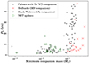 |
Fig. 1. Orbital periods of known spider systems compared against minimum companion masses. In this figure, spider systems are categorised as BW or RB depending on the companion type listed in the ATNF catalogue: Main sequence (MS) stars for RBs or ultra low-mass objects (ULs) in the case of BWs. Some NRT spiders have no information about the companion type in the catalogue; hence, some circles have no cross inside. |
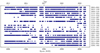 |
Fig. 2. Time span of the NRT dataset considered in this study. Each dot represents an observation made with the NUPPI backend. |
Properties of the NRT dataset used in this study.
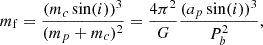
Astrometric, spin and dispersion measure (DM) properties for the 19 pulsars in our sample are listed in Table 2, and basic orbital properties are listed in Table 3. Companion masses in the latter table were derived from the Keplerian parametersusing
Astrometric and spin properties of the 19 pulsars constituting our spider pulsar sample.
Binary properties of the 19 pulsars constituting our spider pulsar sample.
 (1)
(1)
where mf is the mass function, mp (resp. mc) is the mass of the pulsar (resp. companion), i is the orbital inclination, G is the gravitation constant, ap is the semi-major of the pulsar orbit relative to the common centre of mass, and Pb is the orbital period. The companion masses in Table 3 were determined assuming a pulsar mass of 1.5 M⊙. Minimum companion masses were determined using i = 90°, while median values were calculated assuming i = 60°. In the following subsections, we describe some of the main properties of the pulsars in our sample.
2.1. PSR J0023+0923
PSR J0023+0923 was discovered as part of a survey of unassociated Fermi-LAT sources with the Green Bank Telescope (GBT) at 350 MHz (Bangale et al. 2024). It has a period of 3.05 ms, and a DM of 14.32 pc cm−3 putting it at a distance of 1.24 kpc according to the YMW16 model for the distribution of free electrons in the Milky Way (Yao et al. 2017). It has been observed in X-rays (Gentile et al. 2014), and has been detected with the LAT as a pulsed source of γ-ray emission (see e.g. Smith et al. 2023).
It is classified as a BW due to its very typical 0.016 M⊙ minimum companion mass, and short orbital period of 3.3 h. The companion has been observed at optical wavelengths with multiple instruments (Breton et al. 2013; Draghis et al. 2019; Mata Sánchez et al. 2023). The system is not displaying eclipses in the L-band, and is not reported to display eclipses at 350 MHz or 2 GHz (Bangale et al. 2024).
2.2. PSR J0610−2100
PSR J0610−2100 was discovered during the Parkes High-Latitude pulsar survey (Burgay et al. 2006). It has a period of 3.86 ms and a DM of 60.7 pc cm−3 placing it at a distance of 3.26 kpc according to the YMW16 model. It was first reported to emit pulsed γ rays by Espinoza et al. (2013).
It is classified as a BW due to its 0.021 M⊙ minimum companion mass, and short orbital period of 6.9 h. The companion has been detected at optical wavelengths in archival observations obtained with FORS2 (Pallanca et al. 2012). This system is not known to display eclipses.
2.3. PSR J0636+5128
PSR J0636+5128 was found in the Green Bank Northern Celestial Cap Pulsar Survey (Stovall et al. 2014). It has a period of 2.87 ms, and a DM of 11.1 pc cm−3. The YMW16 model predicts a very small distance of 0.21 kpc for this DM and set of sky coordinates. Pulsed γ-ray emission was first detected and reported by Smith et al. (2019). With its ultra-light companion (minimum mass of 0.007 M⊙ ≃ 7.3MJ) and short orbital period of 1.6 h, it is classified as a BW pulsar. Its orbital period is among of shortest currently known among the binary pulsar population.
The companion has been detected in 2014 Gemini archival data (Draghis & Romani 2018). This system is not known to display eclipses. Unlike PSRs J0023+0923 and J0610−2100 that have been observed with NUPPI soon after it was installed in August 2011, NRT observations of J0636+5128 began in late 2013.
2.4. PSR J1124−3653
PSR J1124−3653 was found during a 350 MHz survey of unassociated Fermi-LAT sources with the GBT (Bangale et al. 2024). It has a period of 2.41 ms, and a DM of 44.9 pc cm−3 putting it at a distance of 0.99 kpc according to the YMW16 model. It has been observed in X-rays (Gentile et al. 2014), and is detected to emit pulsed γ-ray emission (Smith et al. 2023).
With its low minimum companion mass of 0.027 M⊙ and short orbital period of 5.4 h, it is a BW pulsar. It is extremely faint in 1.4 GHz NRT observations: as can be seen from Table 1 the median S/N of our observations of this one is only 6.5. Although the pulsar is seen to display eclipses at 1.4 GHz in the NRT data, the very low S/N values prevented us from obtaining satisfactory results for the eclipse analysis using the same analysis method as for the others.
2.5. PSR J1513−2550
PSR J1513−2550 was found in a survey for new pulsars at the locations of Fermi-LAT unassociated sources at 800 MHz with the GBT(Sanpa-Arsa 2016). It has a period of 2.12 ms, and a DM of 46.9 pc cm−3. The YMW16 model of free electrons in the Galaxy places the pulsar at a distance of 3.96 kpc. It has been detected as a pulsed source of γ rays with the LAT (Smith et al. 2023).
It is classified as a BW due to its 0.016 M⊙ minimum companion mass and short orbital period of 4.3 h. At 1.4 GHz this system is observed to eclipse, with short-duration (duty cycles of less than 10% of the orbital period) total eclipses. NRT observations of J1513−2550 began in March 2014.
2.6. PSR J1544+4937
This 2.16 ms pulsar with a DM of 23.2 pc.cm−3 was discovered as part of a search for pulsars in LAT unassociated sources with the GMRT (Bhattacharyya et al. 2013). The YMW16-predicted distance for this DM value is 2.98 kpc. The low minimum companion mass (0.017 M⊙) and short orbital period (Pb ∼ 2.9 h) make it a BW pulsar. The analysis of Fermi-LAT data revealed that J1544+4937 emits pulsed γ-ray emission (Bhattacharyya et al. 2013; Smith et al. 2023).
The companion has been detected in optical (Tang et al. 2014) and is thought to be nearly Roche-lobe filling (Mata Sánchez et al. 2023). This system displays total eclipses at 322 MHz, and the TOAs present significant delays around superior conjunction at 607 MHz, with delays reaching more than 10% of the pulsar’s spin period (Bhattacharyya et al. 2013). The 1.4 GHz NRT data do not appear to reveal any significant delays around superior conjunction. NRT monitoring of this object began in early 2013, soon after the discovery of this pulsar.
2.7. PSR J1555−2908
PSR J1555−2908 was found in a search of Fermi-LAT unassociated sources with the GBT at 800 MHz (Ray et al. 2022). The LAT data analysis revealed that the pulsar also emits pulsed γ-ray emission. This pulsar has a period of 1.79 ms, and a DM of 75.9 pc cm−3. For this DM and line of sight the YMW16 model predicts a distance of 7.55 kpc, making this pulsar the most distant in our sample.
The minimum companion mass of 0.051 M⊙ and short orbital period of 5.6 h make PSR J1555−2908 a BW pulsar. Optical observations constrained the minimum companion mass to be 0.060 ± 0.005 M⊙, placing the system at the upper limit of what is considered a BW (Kennedy et al. 2022). The companion is severely bloated, with a Roche-lobe filling factor (“measured as the ratio of the stars radius to the L1 point along the line joining both”) of f = 0.98 ± 0.02.
PSR J1555−2908 displays eclipses in γ rays. Eclipses at such short wavelengths indicate that the system is seen nearly edge-on, Clark et al. (2023) showed by analyzing Fermi-LAT data that the derived orbital inclination is greater than 83°. Moreover, analysis of the γ-ray eclipses enabled model-independent constraints on the pulsar mass, which are estimated to be mp = 1.645 ± 0.065M⊙. NRT monitoring of PSR J1555−2908 began relatively recently, with first observations conducted in mid-2021.
2.8. PSR J1628−3205
PSR J1628−3205 was discovered in a survey of Fermi-LAT unassociated sources at 350 MHz with the GBT (Ray et al. 2012). Pulsations were later detected in the γ-ray data recorded by the LAT, and reported in Smith et al. (2023). This pulsar has a rotational period of 3.21 ms, and a DM of 42.1 pc cm−3, placing the pulsar at a distance of 1.22 kpc according to the YMW16 model.
Its comparatively larger minimum companion mass of 0.109 M⊙ and short orbital period of 5 h make it a RB pulsar. It is the only RB in our sample. In fact, optical observations by Li et al. (2014) constrained the companion mass to be larger than 0.161 M⊙. Analysis of the 1.4 GHz NRT data does not reveal eclipses around superior conjunction. Routine monitoring of this pulsar with the NRT began in early 2013.
2.9. PSR J1705−1903
PSR J1705−1903 was discovered with the Parkes radio telescope as part of the HTRU survey (Morello et al. 2018). It has a period of 2.48 ms, and a DM of 57.5 pc.cm−3. The YMW16 distance for this DM and line of sight is 2.34 kpc. This pulsar is one of the few in this sample that is not detected in γ rays, yet. It also does not appear to have any γ-ray counterpart. The nearest source from the Fermi-LAT 14-Year Point Source Catalog (hereafter 4FGL; Ballet et al. 2023) is 11’ away and is associated with PSR J1705−1906 (Smith et al. 2023).
It is classified as a BW due to its low minimum companion mass of 0.047 M⊙ and short orbital period of 4.4 h. This system does not display total eclipses in the NRT data at 1.4 GHz, but does display significant delays at superior conjunction. We therefore categorised it as an eclipser. NRT monitoring on this one started in November 2022. The NRT dataset on this pulsar has the shortest time span among the datasets considered in this study.
2.10. PSR J1719−1438
PSR J1719−1438 was discovered with the Parkes radio telescope as part of the HTRU survey (Bailes et al. 2011). It has a period of 5.79 ms, and a DM of 36.8 pc cm−3, placing it at a very close distance of 0.34 kpc according to the YMW16 model. As for PSR J1705−1903, it is currently undetected in γ rays, and there are no 4FGL sources within 1° of the pulsar position.
This system has a peculiar status: it is classified as a BW by default, but has an extremely light companion, with a minimum companion mass of 0.001 M⊙. The companion is believed to be Jupiter-sized but up to ten times denser, around 23 g cm−3. As the companion is likely closer to a planet than it is to a star, it has been suggested that the system could be part of a sub-class of BWs that have a different evolutionary path (Guo et al. 2022), or that it is not a BW at all, but could be the missing link between X-ray binaries and isolated pulsars (van Haaften et al. 2013). It has been searched for in optical (Bailes et al. 2011) but was not detected at the expected magnitude and location.
Computational evolutionary models constrain the companion to be Helium or Carbon rich (Bailes et al. 2011). The exact nature of the companion is yet unknown, but potential progenitors could be a He or C white dwarf (Bailes et al. 2011) or a He star (Guo et al. 2022). This could make PSR J1719−1438 a member of a separate category, different from BWs, in which the companions are usually considered non-degenerate. This system is not known to display eclipses.
2.11. PSR J1731−1847
PSR J1731−1847 was discovered with the Parkes radio telescope during the HTRU survey (Bates et al. 2011). It has a spin period of 2.34 ms, and a DM of 106.6 pc cm−3, the largest in our pulsar sample. The YMW16 distance for this object is 4.77 kpc. Interestingly, the pulsar is located only 6.5′ away from a 4FGL source, 4FGL J1731.7−1850, with no known association. Nevertheless, no γ-ray pulsations have been reported from PSR J1731−1847 yet.
The orbital period is 7.5 h, and the minimum companion mass is 0.033 M⊙, making this object a BW. This system displays eclipses from 1.4 GHz down to at least 700 MHz (Bates et al. 2011).
2.12. PSR J1745+1017
PSR J1745+1017 was discovered with the Effelsberg radio telescope in a search for pulsars at the locations of unassociated Fermi-LAT sources (Barr et al. 2013). It has a rotational period of 2.65 ms and a DM of 24.0 pc cm−3. The YMW16 model places this pulsar at a distance of 1.22 kpc. Unsurprisingly, given the fact that the pulsar was discovered within the confidence region of a LAT source with no known counterpart, the pulsar was detected to emit pulsed γ-ray emission soon after it was discovered (Barr et al. 2013).
With an orbital period of 17.5 h and a minimum companion mass of 0.014 M⊙, it is classified as a BW pulsar. This system is not known to display eclipses.
2.13. PSR J1959+2048
The discovery of the so-called original BW PSR J1959+2048 (also known as B1957+20), was reported in Fruchter et al. (1988) after a detection with the Arecibo telescope in a survey for millisecond pulsars. It has a period of 1.61 ms, and a DM of 21.9 pc cm−3. The YMW16 distance for this pulsar is 1.73 kpc. Pulsed γ rays from this pulsar were detected using LAT data (Guillemot et al. 2012). The latter study also reported on the detection of pulsed X-ray emission using XMM-Newton data, at the 4-σ confidence level. However, new pulsation searches in X-rays using NICER data did not confirm this detection (Ng et al. 2022).
It is classified as a BW, with its 0.022 M⊙ minimum companion mass and 9.2 h orbital period. This system displays eclipses from 430 MHz (Fruchter et al. 1988) up to the L-band frequency range. The detection of eclipses shed new light upon the mechanism spinning up young pulsars to millisecond rotation periods. While radio eclipses of J1959+2048 have been studied thoroughly (see Main et al. 2018; Lin et al. 2023), the pulsar was also observed to eclipse in γ rays (Clark et al. 2023), indicating that the system is seen nearly edge-on: i > 84.1°. Clark et al. (2023) were also able to put constraints on the mass of the pulsar, finding mp = 1.805 ± 0.135 M⊙, a higher value than the canonical 1.4 M⊙, as for J1555+2908, albeit much lower that the initially inferred 2.4 M⊙ (van Kerkwijk et al. 2011).
2.14. PSR J2051−0827
PSR J2051−0827 was the second spider discovered. It was reported in Stappers et al. (1996) after a detection with the Parkes telescope during a survey of the southern sky. It has a spin period of 4.51 ms, and a DM of 20.7 pc cm−3 placing it at a distance of 1.47 kpc according to the YMW16 model.
It is classified as a BW, with its minimum companion mass of 0.027 M⊙ and 2.4 h orbital period. This system displays eclipses from 436 MHz (Stappers et al. 1996) up to the L-band. Polzin et al. (2019) showed that the eclipses are not seen at every orbit, and are variable, in duration and in occurrence. Additionally, the centroid of the eclipse is seen to vary in orbital phase over a year-long period (see Fig. 4 of Polzin et al. 2019, for a comprehensive plot of Effelsberg observations of J2051−0827 eclipses). Although these properties are unique among spider pulsars, this uniqueness is to be taken with caution, given the fact that PSR J2051−0827 has been studied much more extensively than most other spider pulsars. PSR J2051−0827 is also known to display rapid variations of its orbital properties (Shaifullah et al. 2016) that might be linked to the above-mentioned variability of the eclipses. Changes in rotation measure during the eclipse (Wang et al. 2023b) and intra-system plasma lensing (Lin et al. 2021) have also been reported for this pulsar. This is also the first (and to this date only) system for which the quadrupole moment of the companion has been measured (Voisin et al. 2020). PSR J2051−0827 has been detected to emit pulsed γ-ray emission (Wu et al. 2012; Smith et al. 2023), and its companion has been detected at optical wavelengths (Dhillon et al. 2022).
2.15. PSR J2055+3829
PSR J2055+3829 was discovered at 1.4 GHz as part of the SPAN512 survey conducted with the NRT (Guillemot et al. 2019). It has a spin period of 2.09 ms, and a DM of 91.9 pc cm−3. The YMW16 distance for this DM and line of sight is 4.59 kpc. The pulsar has not been detected as a pulsed source of γ-ray emission, and there are no γ-ray sources within 1° of the pulsar position in the 4FGL catalog.
It is classified as a BW, with a minimum companion mass of 0.027 M⊙ and an orbital period of 2.4 h. As can be seen from Fig. 4 of Guillemot et al. (2019), PSR J2055+3829 is observed to display total eclipses at 1.4 GHz. It has been observed with the NRT since late-2015 with an average observation cadence of one observation every 5.5 days.
2.16. PSR J2115+5448
PSR J2115+5448 was discovered with the GBT at the location of a Fermi-LAT unassociated source (Sanpa-Arsa 2016). It has a spin period of 2.60 ms, and a DM of 77.4 pc cm−3, for which the YMW16 model predicts a distance of 3.11 kpc. The pulsar was detected to produce pulsed γ-ray emission by analysing LAT photons (Smith et al. 2023).
It is classified as a BW, with its minimum companion mass of 0.022 M⊙ and short orbital period of 3.2 h. Analysis of the NRT data reveals that the pulsar displays variable eclipses around superior conjunction, with the radio signal being totally eclipsed during some orbits, and only delayed during others. Routine monitoring of this pulsar with the NRT began in mid-2015.
2.17. PSR J2214+3000
This pulsar was discovered by Ransom et al. (2011) at the location of a Fermi-LAT source with no known counterparts. It was quickly detected as a pulsed source of γ-ray emission, confirming that it was indeed powering the LAT unassociated source. It has a spin period of 3.12 ms, and a DM of 22.6 pc cm−3 placing the system at a distance of 1.68 kpc according to the YMW16 model.
Its orbital period of 10 h and minimum companion mass of 0.007M⊙ make it a BW system. First detection of the companion has been reported by Schroeder & Halpern (2014). It has not been reported to display eclipses, and the analysis of the 1.4 GHz NRT indeed did not yield any eclipse detection.
2.18. PSR J2234+0944
PSR J2234+0944 was discovered at the location of a Fermi-LAT unassociated source with the Parkes radio telescope (Ray et al. 2012). It was later confirmed to emit pulsed γ-ray emission (see e.g. Smith et al. 2023).
It has a spin period of 3.63 ms, a DM of 17.8 pc cm−3, an orbital period of 10 h and a minimum companion mass of 0.008 M⊙. The YMW16 model places this pulsar at a distance of 1.58 kpc. This pulsar’s orbital properties make it a BW-type object. Investigation of the 1.4 GHz NRT data did not reveal the presence of eclipses, and the pulsar has not yet been reported to display eclipses at other frequencies.
2.19. PSR J2256−1024
PSR J2256−1024 was discovered with the GBT as part of a drift scan survey at 350 MHz (Crowter et al. 2020). It has a spin period of 2.30 ms, and a DM of 13.8 pc cm−3. The YMW16 model of free electrons in the Galaxy predicts a distance of 1.33 kpc for this direction and DM value.
The pulsar has been observed in X-rays (Gentile et al. 2014) and has been detected to emit pulsed γ-ray emission (Smith et al. 2023). Optical observations of the system yielded a detection of the companion object (Breton et al. 2013). The pulsar is seen to exhibit total eclipses in the 1.4 GHz NRT data.
3. Eclipse analysis
3.1. Data preparation and timing analysis
In order to characterise the properties of the eclipses detected in the 1.4 GHz NRT data, we started by conducting timing analyses of all the selected pulsars, to construct timing solutions enabling us to determine pulsar orbital phases with good accuracy.
The NUPPI data on the selected pulsars were cleaned of radio-frequency interference (RFI) using the SURGICAL method of the COASTGuard pulsar analysis library (Lazarus et al. 2016). The PSRCHIVE software library (Hotan et al. 2004) was used to calibrate the polarisation information, and to perform all subsequent data reduction steps.
The timing analysis was done in two steps. We first constructed reference profiles for each of the considered pulsars by summing up eight time- and frequency-averaged observations with high S/N values, and smoothing the obtained integrated profiles. We then extracted TOAs from the individual observations by cross-correlating them with the reference profile for the corresponding pulsar. In this first step, the cross-correlations were performed using the Fourier domain with Markov chain Monte Carlo algorithm implemented in the pat routine of PSRCHIVE. We generated one TOA per 64 MHz of frequency bandwidth in order to track time variations of the DM and one per 5 min for the TOAs to cover less than a few percent of the pulsar’s orbital period. The TOA data were analysed using the TEMPO2 pulsar timing suite (Hobbs et al. 2006). We discarded TOAs around superior conjunction in the case of pulsars observed to display eclipses in the NRT data. We then obtained timing solutions for each pulsar by fitting the timing residuals (i.e., the differences between measured arrival times and those predicted by TEMPO2) for their spin, astrometric, DM and orbital parameters. DM variations were modelled by fitting for up to two time derivatives, and similarly variations of the orbital period, which are commonly observed in these systems, were fitted for by including up to 17 derivatives (in the case of PSR J2051−0827).
In the second step of the timing analysis, we used the timing solutions obtained from the previous analysis step to refold all individual observations, and formed 2D template profiles from archives with 8 frequency sub-bands of 64 MHz each for each pulsar. For pulsars with observations that have S/N values larger than 100, we used the highest-S/N observation as the 2D template. For the other pulsars we summed up the three highest-S/N observations to form the 2D template. With these standard profiles with frequency resolution we could follow the same analysis procedure as in Guillemot et al. (2019) and use the wide-band template-matching technique implemented in the PulsePortraiture library (Pennucci et al. 2014) to extract one TOA per 10 min of observation for the entire bandwidth. Extracting TOAs using the 2D template-matching method implemented in the PulsePortraiture toolkit has several advantages: first of all, as can be seen from Table 1, many of the pulsars in our sample are detected with low S/N values at 1.4 GHz with the NRT. For observations near the detection limit, using the usual pat routine to determine one TOA per frequency-band of 64 MHz can result in a large number of outlier TOAs. In Table 4 we list the fraction of TOA outliers as obtained with the 1D and 2D TOA extraction methods. Extracting TOAs with the wideband-matching technique results in lower outlier rates in all cases, and in some cases (see e.g. PSR J1513−2550 or J2055+3829) the outlier rate decreases dramatically when using the 2D template-matching method.
Fraction of outliers in the TOA datasets.
Second, in some pulsars the pulse profile is observed to vary significantly with frequency, as is illustrated in Fig. 3 for PSR J0023+0923. For these pulsars, TOAs determined using the 2D template-matching method are more accurate than TOAs extracted using a single frequency-averaged profile for the entire band. Finally, as mentioned in Guillemot et al. (2019), in addition to determining a single TOA for the entire available bandwidth in a given time sample, the PulsePortraiture library also determines a DM value by comparing the reference profile and the 2D profile in the considered time sample, theoretically enabling us to investigate short-term variations of the DM around superior conjunction. However, in our sample, the majority of the pulsars are too faint to give satisfactory DM measurements. Hence, we decided to conduct the following study on the TOAs only. After the latter analysis step, we obtained TOA and DM datasets for each pulsar in the sample, with one measurement per 10 min of observation. In the next subsection we present a phenomenological analysis of the eclipses properties of the pulsar in our sample, using these TOA datasets.
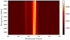 |
Fig. 3. Two-dimensional template profile of PSR J0023+0923 as determined using the PulsePortraiture software suite. The sub-components of the main pulse of this pulsar were observed to evolve with frequency, with the first one being brighter than the second at lower frequencies and fainter at the top of the observed bandwidth. When collapsed in frequency, this profile displays two equally bright peaks. |
3.2. Eclipse characterisation
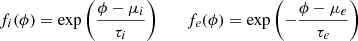
Depending on the precise geometry of the systems, the radio signal from eclipsing spider pulsars can disappear or get attenuated over a certain phase interval around superior conjunction. The TOA extraction procedure described in Sect. 3 determined TOAs in every 10-min sample of the pulsar observations, meaning independently of whether the pulsar is detected or not. The procedure also determines a S/N associated which each TOA, therefore providing a way of discriminating eclipsing and non-eclipsing spiders: around superior conjunction, pulsars exhibiting eclipses are expected to be detected with lower S/N values than well away from superior conjunction, whereas pulsars that do not have eclipses should be detected with similar S/N values throughout their orbit. Figure 4 shows timing residuals and S/N values as a function of orbital phase for PSR J2055+3829.
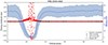 |
Fig. 4. Timing residuals and median S/N values as a function of orbital phase for PSR J2055+3829. The TOA residuals are shown as red and black dots, with red dots corresponding to observations with S/N values among the 25% lowest. Error bars, which are much smaller than the vertical scale, are not visible in this figure. The blue curve is the median S/N of the TOAs computed over sliding windows of width 0.1 in orbital phase, and the blue zone shows the median absolute deviation around the median values. The dashed vertical line corresponds to superior conjunction, at orbital phase 0.25. |
It should be noted that the data points shown in Fig. 4 were recorded over a very large number of pulsar orbits, and highly sensitive observations of spider pulsars have shown that the eclipse properties of some objects vary from one orbit to another (Polzin et al. 2019). Figure 4 therefore shows the “average” eclipse properties of PSR J2055+3829 in our dataset. Nevertheless, median S/N values for this pulsar are clearly seen to drop around superior conjunction. We thus define PSR J2055+3829 as being an eclipsing pulsar in the 1.4 GHz NRT data, and generally define eclipsing pulsars as those displaying S/N drops around superior conjunction. In Figs. A.1 to A.3 we show plots of the S/N values as a function of orbital phase for all the pulsars in our sample.
From these plots we classify eclipsers and non-eclipsers as follows: a pulsar is considered an eclipser when the median S/N at superior conjunction is lower than the median S/N of ϕ > 0.5 minus the median absolute deviation. With this definition, eight out of 19 spiders of the sample are eclipsers. Those eight pulsars display what we call “total” eclipses, during which the beam is not detectable for a few sub-integrations, leading to very low S/N TOAs. In addition, around superior conjunction the residuals of the eclipsers display a significant delay, typically around 5 to 8% of the spin period. These TOAs are usually associated with S/N values lower than those of TOAs well away from the eclipse region, but still higher than the threshold we defined to determine non detections. The additional delay in TOAs that correspond to detections is due to the additional plasma crossing the line of sight.
Nevertheless, three pulsars in our sample display eclipsing behaviour in our data, without strictly respecting the criteria mentioned above for defining eclipsing pulsars. PSR J1124−3653, whose TOA residuals around superior conjunction are not distributed around zero unlike in other orbital phase ranges, appears to display eclipses. However, it is too faint for our eclipse analysis to yield satisfactory results. PSR J1705−1903 displays “shallow” eclipses: the S/N drop for this pulsar is less pronounced than in other pulsars due to the fact that its radio beam is detectable throughout the orbit. Yet, residuals around superior conjunction clearly depart from zero up to approximately 0.5% of its spin period, albeit much less strongly than in other eclipsers. Because the beam is eclipsed by plasma, the eclipsing mechanisms are frequency dependent, and eclipses are more pronounced at lower frequencies compared to higher frequencies. This also means that the frequency below which the pulsed signal disappears, called the cut-off frequency, varies from one pulsar to another (it can also vary with time, see e.g. Kumari et al. 2024, for a detailed study of the variation of the eclipse cut-off frequency in PSR J1544+4937). The cut-off frequency in PSR J1705−1903 appears to be lower than that of most known eclipsers, at a frequency below 1.2 GHz. No observations of this pulsar at these low frequencies have been reported, to the best of our knowledge. The third pulsar, PSR J2051−0827, does not display any drop in S/N around superior conjunction. However, its TOA residuals depart from zero, indicating that extra material is traversed by the radio beam. PSR J2051−0827’s eclipses therefore also appear to have a cut-off frequency below 1.2 GHz. This pulsar has been observed thoroughly and displays total eclipses at 660 MHz (Stappers et al. 1996). In conclusion, PSRs J1124−3653, J1705−1903 and J2051−0827 are still considered eclipsers in the rest of the paper, and are flagged as such in Table 3. However, due to the above-mentioned peculiarities, the phenomenological fits presented in the following section did not yield satisfactory results for the very faint pulsar J1124−3653, and did not produce optimal results for PSRs J1705−1903 and J2051−0827, due to the lack of clear, total eclipse phases in the data for these objects.
As mentioned above, the TOA extraction procedure determined TOAs for every 10 min sample, regardless of whether the observed pulsar is indeed detected in the considered time sample or not. The TOAs in these time samples corresponding to non-detections therefore needed to be discarded from our datasets. We again made selections in our timing datasets based on the S/N values associated with the TOAs: as can be seen from Fig. 4, TOAs with S/N values among the 25% lowest are mostly located in the orbital phase interval corresponding to the eclipse. For the 10 eclipsing pulsars we discarded TOAs associated with S/N values within the first quartile. This threshold of 25% was chosen as a compromise for the ten considered objects, between the need to eliminate data points corresponding to non-detections while keeping large enough numbers of data points.
We finally modelled the timing residuals of the pulsars in our sample to determine their average eclipse properties, following a phenomenological approach. This analysis is presented in the following subsection.
3.3. Phenomenological modelling
For each of the ten pulsars found to display eclipses in the NRT data, we fitted the timing residuals cleaned of the 25% lowest S/N detections to a symmetrical function over a background level:
 (2)
(2)
with
 (3)
(3)
and H as the Heaviside step function: H(x) = 
In the above expressions, b is the background level, corresponding to the average timing residual value away from the eclipse, and the fi and fe are the functions used to fit the timing residuals in the ingress and egress phases. Each of the two functions has two parameters: a centroid μ and a characteristic phase τ. Five parameters were therefore fit for each pulsar: b and the μ and τ parameters. The function for the ingress part is fitted to timing residuals at orbital phases from 0 to 0.25, and that for the egress part is fitted to residuals at orbital phases from 0.25 to 0.5. The parameter space was explored using a parallelised affine-invariant Monte Carlo sampling algorithm implemented in the EMCEE library (Foreman-Mackey et al. 2013). Figure 5 shows an example of timing residuals as a function of orbital phase around superior conjunction for PSR J2055+3829, along with the best-fit function found from this analysis. Figures showing the fit results for the other analysed pulsars can be found in Appendix B. Results of the fits are summarised in Table 5.
 |
Fig. 5. Timing residuals as a function of orbital phase around superior conjunction, indicated with a solid line for PSR J2055+3829. The best-fit function obtained from the analysis presented in Sect. 3.3 is shown in red. The light red zone shows the RMS of the timing residuals for orbital phases ϕ > 0.5, and the dashed vertical lines correspond to the values of Φstart and Φend as inferred from the fit. |
From this fit we determined two additional parameters, the values of which are collected in Table 5: Φstart, the orbital phase at which the ingress phase begins, and Φend, the orbital phase at which the egress phase ends. Between Φstart and Φend, the best-fit function is above b + σ, with σ denoting the standard deviation of the timing residuals away from the eclipse phase (in this case, we considered orbital phases larger than 0.5). For “abrupt” eclipses, no data points could be fit in the ingress phase. In these cases, Φstart was defined as the orbital phase of the last valid data point before superior conjunction.
Parameters of the functions describing the eclipse ingress and egress phases.
Measuring Φstart and Φend enabled us to determine eclipse duty cycles, Tdelay, as Tdelay = Φend − Φstart. For each pulsar we also determined Tobsc, corresponding to the phase interval over which the pulsar is completely eclipsed in our data, which is the duration between the leftmost point with ϕ > 0.25 and the rightmost point with ϕ < 0.25. Values of Teclipse and Tobsc from our analysis are listed in Table 6. In this Table, the values of Tdelay and Tobsc are expressed in fraction of the orbital period and in time. In Table 6 we also list slope ratios S = τi/τe, and ingress/egress duration ratios D, calculated as D = (0.25 − Φstart)/(Φend − 0.25). The closer D is to 1, the more symmetric the eclipse is, and conversely.
Parameters derived from the results of the fit of pulsar eclipse properties.
The parameter Tobsc/Tdelay is the fraction of the eclipse phase over which the beam is not detectable. The closer to one this parameter is, the shorter the ingress and/or egress phases are before and/or after the flux drops below the detection level. Conversely, a value of zero indicates that the beam is detectable throughout the eclipse.
4. Polarimetry
In addition to determining the eclipse properties of the pulsars in our sample that display eclipses in the 1.4 GHz NRT data, we also characterised the polarimetric properties of these pulsars. To construct polarimetric profiles for the 19 pulsars, we selected 1.4 GHz NUPPI observations conducted after MJD 58800 (13 November 2019), which are observations that can be polarisation calibrated using the improved calibration scheme presented in Guillemot et al. (2023). For pulsars displaying eclipses we only considered data taken away from the eclipse regions. Individual observations, prepared with the same procedure as described in Sect. 3.1, were summed in time using the psradd tool of PSRCHIVE, to form high S/N polarimetric profiles. For pulsars with Rotation Measure (RM) information available in the ATNF pulsar catalogue, we corrected the polarimetric profiles from Faraday rotation of the polarisation position angle across the bandwidth. For the other five pulsars (namely, PSRs J1124−3653, J1513−2550, J1555−2908, J1628−3205, J2115+5448), no RM information was available in the ATNF catalogue at the time of writing. We attempted to determine RM values from the summed NUPPI polarimetric profiles, but the low degrees of linear polarisation in these pulsars and very low S/N values in some cases prevented us from determining the RMs. The summed observations were finally scrunched in frequency.
The resulting polarimetric profiles at 1.4 GHz for the 19 pulsars in our sample are shown in Figs. C.1 to C.3. Pulsar profiles that were not corrected for Faraday rotation are marked with a star. We note that the 1.4 GHz polarimetric profiles of PSRs J1124−3653, J1555−2908, J1628−3205, and J2115+5448 were previously unpublished, to the best of our knowledge. Polarimetric profiles for the other pulsars are consistent with the previously published ones. In Table 7 we list the pulsar RMs, and values of the polarised intensities and linear, circular and absolute circular intensities, as determined using the psrstat tool of PSRCHIVE. For pulsars for which we lacked an RM value and thus could not correct the data for Faraday rotation, we do not quote the polarised intensities and linear intensities. Polarisation fractions vary broadly across the sample, with values ranging from 13% to 66%.
Polarisation parameters for the 19 pulsars in our sample.
In order to put our polarisation fraction measurements in a broader context, we plotted in Fig. 6 the linear and absolute circular polarisation fractions listed in Table 7 along with the measurements for 682 pulsars published in Wang et al. (2023a), obtained using the Five-hundred-meter Aperture Spherical radio Telescope (FAST). One can see on this figure that most spider pulsars appear to have low degrees of polarisation, similarly to non-spider MSPs. It can also be noted that NRT measurements are complementary to those of Wang et al. (2023a) and display similar trends. We performed 2D Kolmogorov-Smirnov tests using the publicly available software NDTEST3, to compare the polarisation fractions of spider pulsars with those of other MSPs and slow pulsars. For spider pulsars we combined NRT and FAST polarisation measurements, leading to a sample of 26 objects with linear and absolute circular polarisation fractions. The other samples included 66 non-spider MSPs, and 582 slow pulsars. We found a probability that polarisation data for spider MSPs and slow pulsars originate from the same parent distribution of approximately 8.5%, suggesting that the two populations have distinct polarisation properties. On the other hand, the test found a larger probability of ∼20% that the data for spider and non-spider MSPs originate from the same parent distribution, thus preventing us from drawing any conclusions.
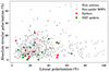 |
Fig. 6. Linear polarisation fractions and absolute circular polarisation fractions for the 682 pulsars from Wang et al. (2023a). Grey diamonds are slow pulsars, and grey dots represent isolated MSPs or MSPs in non-spider systems (pulsars orbiting white dwarf companions or main sequence stars). Red stars are spiders that are not in the NRT sample, and green stars are the spiders analysed in this article. The values for the latter objects can be found in Table 7. |
5. Analysis of eclipse and pulse profile properties
5.1. Correlations between eclipse parameters
Two categories of eclipsers can be distinguished in Figs. B.1 and B.2, in addition to the “shallow” eclipsers PSRs J1705−1703 and J2051−0827. On the one hand, eclipsing pulsars displaying no ingress phases, for which the S/N cut-off left no TOAs forming an ingress slope outside the red zone (RMS of TOA residuals far from the eclipse), namely PSRs J1513−2550, J1555−2908 and J2115+5448, and on the other hand, pulsars with a progressive ingress phase, namely PSRs J1628−3205, J2055+3829 and J2256−1024. It is worth noting that two pulsars lie in a grey area between the earlier two categories: PSRs J1731−1847 and J1959+2048. PSR J1731−1847 is the least observed eclipser in our sample, and very few TOAs remained after data selection, making it difficult to probe the ingress region and search for a proper slope in that region. Unlike PSR J1731−1847, the data selection left numerous TOAs in the ingress phase of PSR J1959+2048. However, this one displays a very steep ingress and is seen to eclipse in gamma rays (Clark et al. 2023), similarly to PSR J1555−2908 which also displays an “abrupt” ingress phase. For these reasons, the two pulsars are represented with different colours than others in Figs. 7 and 8.
 |
Fig. 7. Obscuration duration (Tobsc) against delay duration (Tdelay). The grey zone line is the 1:1 line. An eclipsing pulsar on this line would have no ingress and egress phases. The further a pulsar is from this line, the smaller is the fraction of the eclipse over which the beam is not detectable. Colours and shapes depend on the classifications, as given in Table 6: blue circles correspond to the “abrupt” eclipsers, PSRs J1513−2550, J1555−2908 and J2115+5448, red diamonds are the “progressive” eclipsers, PSRs J1628−3205, J2055+3829 and J2256-1024 and green stars are the “shallow” eclipsers, namely PSRs J1705−1903 and J2051−0827. |
 |
Fig. 8. Ingress/egress duration ratio D and ingress/egress slope ratio S as a function of the Tobsc/Tdelay ratio. This ratio is the fraction of the orbit over which the radio beam of the pulsar is not detectable. Values of S and D can be found in Table 6. Colours and symbols are the same as in Fig. 7. |
Looking at Table 6, we can notice that eclipse durations (Tdelay) vary widely, ranging from 8.3% up to 37% of the respective orbital periods, as do the obscuration durations (Tobsc), that range from 0% to 21.5% of the orbital period. These two parameters do not appear to be strongly correlated, as can be seen from Fig. 7. Nevertheless, it appears from this figure that Tobsc seems to be closer to Tdelay for “abrupt” eclipsers, represented as blue circles, than for those classified as being “progressive” eclipsers, shown with red diamonds. In this regard, PSR J1731−1847 bears resemblance to “abrupt” eclipsers, while PSR J1959+2048 shows similarities with “progressive” eclipsers.
In addition, it can be seen from Table 6 that most duration ratios D are found to be smaller than one for this pulsar sample, meaning that these objects have longer egress phases than ingress phases. This is not the case for PSRs J1705−1903 and J2055+3829, as can be seen from Fig. B.1: the eclipses of these pulsars are asymmetric but with longer ingress phases.
From the upper panel of Fig. 8 we can notice a very rough trend of negative correlation between the symmetry parameter D and the fraction of the eclipse over which the beam is not detectable, Tobsc/Tdelay, with abrupt eclipsers displaying larger Tobsc/Tdelay and lower D values, progressive eclipsers having intermediate Tobsc/Tdelay and D values, and shallow eclipsers having high D values and null Tobsc/Tdelay ratios. The difficulty to assign PSRs J1731−1847 and J1959+2048 one of the classifications given in Table 6 is clear from this figure, since PSR J1731−1847 has a high Tobsc/Tdelay value and an intermediate D value, while PSR J1959+2048 has an intermediate Tobsc/Tdelay value and a low D ratio. This porosity between the two categories is not surprising, because of the strong frequency dependence of eclipsing behaviour: for instance, some pulsars classified as “progressive” eclipsers at 1.4 GHz could appear as “abrupt” eclipsers at lower frequencies, where eclipses become more abrupt and obscuring phases become longer. It could be that the three categories we have distinguished in fact belong to a spectrum of eclipse behaviours.
Finally, slope ratios S are found to be smaller than 1 in almost all cases, corresponding to ingress phases that are generally steeper than the egress phases. In the case of the “abrupt” eclipses, values of the S parameter have large uncertainties. For these objects, the S/N cut left no TOAs in the ingress region, resulting in ingress slopes being difficult to measure accurately. The fit found slope values of 0.01 ± 0.01, leading to uncertain S parameter values. Otherwise, we note from the lower panel of Fig. 8 that the ingress/egress slope ratio S shows, similarly to the D parameter, a trend of negative correlation with the fraction of the eclipse over which the beam is not detected, Tobsc/Tdelay; however the sample is too limited to be conclusive.
5.2. Relationship between eclipsing behaviour and mass function
Comparing properties of BW systems, Freire et al. (2005) found evidence for eclipsing binaries having higher mass functions than non-eclipsing ones. Since the mass function scales as sin(i)3, this could be interpreted as eclipsing systems being seen with higher orbital inclinations. After the numerous discoveries of new BW systems over the last 15 years, Guillemot et al. (2019) re-investigated the mass functions of these systems (see Fig. 6 in the latter article and discussions therein), finding that the mass function distributions of eclipsing and non-eclipsing objects only have ∼0.007% probability of originating from the same parent distributions. We here investigate whether the same trend holds for the pulsars in our sample.
5.2.1. Mass function distribution for eclipsers and non-eclipsers
Freire et al. (2005) and Guillemot et al. (2019) focused on BW pulsars in their studies. Similarly, our pulsar sample comprises BW pulsars only, with two notable exceptions: first, PSR J1628−3205, which is a RB pulsar and therefore has the heaviest mass function among the sample (see Table 3). Given that the mass function scales as mc3, and since the masses of RB companions are roughly an order of magnitude larger than those of BW companion objects (by definition of the two categories, see Fig. 1), the mass functions of RBs are roughly three orders of magnitude heavier than those of BWs. On the other hand, the median companion mass of PSR J1719−1438 is about an order of magnitude lighter than those of other BWs (see Table 3 and Sect. 2.10 for more details), so that this object has the lowest mass function among the pulsars in our sample, by two orders of magnitude.
With these caveats in mind, in Fig. 9, we compare the mass functions of non-eclipsing pulsars with those of the eclipsing ones for the pulsars in our sample. PSRs J1719−1438 and J1628−3205 are located at the two extremes of the distribution plotted in Fig. 9. The one-dimensional Kolmogorov-Smirnov (KS) test (Press et al. 1992) indicates a probability of ∼0.08% for eclipsing and non-eclipsing pulsars, excluding PSRs J1719−1438 and J1628−3205, to originate from the same parent distributions. Our results are thus in agreement with the conclusions of Freire et al. (2005) and Guillemot et al. (2019).
 |
Fig. 9. Mass function distributions for the pulsars in our sample. |
5.2.2. Dependence of eclipse parameters on mass function
In Sect. 5.2.1 we showed that the non-eclipsing pulsars in our sample tend to have lower mass functions than the eclipsing ones, suggesting that eclipsing pulsars are indeed seen with higher inclinations. Beyond the detection or non-detection of radio eclipses at superior conjunction, the coherent analysis of the eclipse properties of the pulsars in our sample, as presented in Sect. 3.3, provides an opportunity to address the question of the dependence of eclipse parameters on viewing geometry. More specifically, lower inclinations should result in less eclipsing material crossing the line of sight, leading to shorter eclipses, if any.
In Fig. 10 we plot a number of eclipse parameters determined from the analysis described in Sect. 3.3, against mass function. We observe no particular trends in the Tobsc, Tobsc/Tdelay, and duration ratio D parameters as a function of mass function. This is confirmed by the Spearman correlation coefficients (Spearman 1904) of 0.5 found for these three panels, indicating a low to moderate (Hinkle et al. 1979) correlation. We also observe no particular differences in this figure between the three classes of eclipsing systems, other than those already mentioned in Sect. 5.1.
 |
Fig. 10. Eclipse parameters as determined from the phenomenological fits made in Sect. 3.3 as a function of mass function values. As in Figs. 7 and 8, we respectively represent ‘abrupt’, ‘progressive’ and ‘shallow’ eclipsers with circles, diamonds, and stars. Crosses represent non-eclipsing systems. |
However, the top-left panel of Fig. 10 hints at a linear correlation between Tdelay, the total duration of the eclipse, as a function of mass function. In this panel we included PSR J1124−3653, which is seen to eclipse but for which, as mentioned in Sect. 3.2, our phenomenological fits did not yieldsatisfactory results. From a visual inspection of Fig. A.1 we conservatively estimated Tdelay to be about 15 ± 5% of the orbital period. For the sub-sample of 10 eclipsing BWs (excluding the RB pulsar J1628−3205), we find a Spearman correlation coefficient (Spearman 1904) of 0.6. This coefficient indicates a moderate correlation, with a p-value of ∼10%, the p-value in this test being the probability of an uncorrelated system producing datasets that have a Spearman correlation at least as high. With the entire sample of 17 objects (10 eclipsers and 7 non-eclipsers, excluding PSRs J1719−1438 and J1628−3205), and setting Tdelay to 0 for non-eclipsing systems, the coefficient becomes 0.8, with a p-value of ∼0.04%. This high correlation coefficient seems to suggest that eclipsing pulsars with lower mass function values have shorter eclipses, and vice versa, as could be expected under the hypotheses mentioned above. A larger pulsar sample is required to confirm this possible trend.
Published orbital inclinations and Roche-lobe filling factors for the pulsars in our sample.
5.3. Dependence of eclipse parameters on orbital inclination
In Sects. 5.2.1 and 5.2.2 we searched for correlations between eclipse properties and mass function values, arguing that since the mass function scales as sin3i, it can be used as a proxy for the orbital inclination. However, for some of the pulsars in our sample, actual orbital inclination measurements have beenpublished.
We conducted a comprehensive review of published orbital inclination measurements for these objects. The results from our literature review are listed in Table 8. The majority of the orbital inclination measurements listed in this table have been obtained from optical measurements, fitting a heating model to the light curve of the companion object. Several parameters can be inferred from these analyses, including the inclination of the system, and the Roche-lobe filling factor (denoted f in the Table) of the companion object. The other orbital inclination constraints listed in Table 8 were obtained by fitting the eclipses seen in radio (Du et al. 2023) or γ rays (Clark et al. 2023) or radio (Du et al. 2023). As can be seen from the table, for some pulsars multiple i and/or f measurements were available in the literature; measurements that are in some cases inconsistent. For four of the eclipsing pulsars in our sample (PSRs J1513−2550, J1705−1903, J1731−1847 and J2115+5448) no inclination or Roche-lobe filling factor constraints have been published, and for two objects (PSRs J2055+3829 and J2256−1024) we found inclination measurements, but no measurements of f.
In Fig. 11 we plot the eclipse parameters presented in Sect. 5.1 as a function of orbital inclinations i and Roche-lobe filling factors f found in the literature. Both eclipsers and non-eclipsers are shown in Fig. 11, with fit parameters set to 0 in the case of non-eclipsers. In cases where multiple i and/or f constraints were available, we plotted each individual measurement. We note that the inclinations and Roche-lobe filling factors of non-eclipsing pulsars almost span the entire allowed ranges, albeit with large uncertainties.
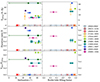 |
Fig. 11. Comparison between the results of the phenomenological fits made in Sect. 3.3 and summarised in Table 6 and the published inclinations and Roche-lobe filling factors listed in Table 8. The symbols are the same as in Figs. 7 and 8: circles correspond to the ‘abrupt’ eclipsers, diamonds are the ‘progressive’ eclipsers, and stars are the ‘shallow’ eclipsers. Crosses are for non-eclipsing systems. |
Contrary to Fig. 10, no obvious link can be found between the eclipse parameters we determined and the orbital inclinations and/or Roche-lobe filling factors. This is aggravated by the fact that few of the eclipsers in our sample have i and f measurements, with only six of the eclipsers having measured orbital inclinations and four having Roche-lobe filling factor estimates. The sample of four objects with both i and f estimates is too small to draw any conclusions at present, but it can serve as a starting point for future studies, when more radio and/or optical studies of eclipsing spiders have been conducted.
5.4. Correlations between mass functions and profile widths
In the simple cone emission model (Lorimer & Kramer 2004), the pulse width W can be written as
 (4)
(4)
where ρ denotes the beam width, α is the angle between the magnetic axis and the spin axis, β is the impact angle of the closest approach of the line of sight to the magnetic axis and ζ = α + β is the angle between the spin axis and the line of sight. In this description, observable pulsars have |β|< ρ, indicating that β needs to be small, and thus, the α and ζ angles need to be similar. Additionally, the long timescale of mass transfer in low mass X-ray binaries is expected to align the spin axis of recycled pulsars with the orbital angular momentum vector (Hills 1983; Bhattacharya & van den Heuvel 1991), leading to ζ ∼ i for recycled pulsars. Furthermore, as mentioned above, the mass function scales as sin(i)3 and can thus serve as a proxy for the orbital inclination. As can be seen from Eq. (4), pulsars with small α values are expected to have broad pulses, under the simple cone model. Therefore, under the various hypotheses mentioned above, we might expect pulse profiles to be narrower for higher mass functions. An important caveat is, of course, the fact that although normal radio pulsars generally have profiles that are adequately represented with the simple cone model, pulse profiles of MSPs are often complex, as can be seen from Figs. C.1 to C.3.
In Fig. 12 we show the equivalent pulse profile widths, weq, where weq corresponds to the width of a rectangle with a height equal to the profile maximum, and whose area is equal to that of the profile, and the profile width at 10% of the maximum, w10, as a function of mass functions. Values of weq and w10 were determined using the profiles shown in Figs. C.1 to C.3. We find Spearman correlation coefficients for the data shown in the top and bottom panels of −0.6 and −0.5, corresponding to low p-values of chance occurrence of ∼2% and ∼5%, respectively. These marginally significant correlations are to be confirmed with more pulsars, and need to be taken with a grain of salt, considering the number of hypotheses made and the caveats mentioned above. We finally searched for correlations between polarisation position angle slopes and mass functions, using the polarimetric profiles shown in Figs. C.1 to C.3, and found none.
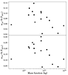 |
Fig. 12. Equivalent width (top panel) and width at 10% of the maximum (bottom panel) as a function of the mass function. The PSRs J1719−1438 and J1628−3205 are not shown for the reasons stated in Sect. 5.2, and PSR J1124−3653 is also not plotted, as the noise baseline in its pulse profile is higher than 10% of the maximum intensity (see Fig. C.1). |
6. Summary and conclusions
In this article, we have presented an analysis of 19 spider-type pulsars observed using 1.4 GHz data taken with the NUPPI backend of the Nançay Radio Telescope. For the majority of the 19 objects, the datasets we analysed spanned more than 12 years; that is, these datasets include NUPPI data taken since this instrument started operating in 2011.
To search the data for the presence of eclipses at superior conjunction caused by outflowing material from the companion, we extracted TOAs from the NUPPI data using the 2D template-matching technique implemented in PulsePortraiture. This approach enabled us to obtain reliable timing data for all the considered pulsars, including for the pulsars with the lowest S/N detections. Additionally, the TOA datasets obtained using PulsePortraiture generally presented lower outlier rates than datasets constructed using the standard template-matching method and fully or partially frequency-scrunched observations. We then conducted a timing analysis for each of the considered pulsars, which enabled us to properly determine the orbital phases associated with each of the TOAs over the entire time spans of the datasets.
Our analysis of the S/N values associated with the TOAs across the orbits revealed that eight of the 19 spider pulsars in the sample display ‘total’ eclipses, namely, PSRs J1513−2550, J1555−2908, J1628−3205, J1731−1847, J1959+2048, J2055+3829, J2115+5448, and J2256−1024. We also found that two pulsars display ‘shallow’ eclipses, during which the pulsar does not become entirely obscured: PSRs J1705−1903 and J2051−0827. Finally, we found that PSR J1124−3653 also appears to display eclipses but is too faint for the eclipse properties to be constrained adequately with the NRT data. In total, we found that 11 of the 19 spider pulsars in our sample display eclipses around superior conjunction at 1.4 GHz, while the remaining eight pulsars do not appear to display eclipses at these frequencies.
We conducted a phenomenological fit of the TOA residuals around superior conjunction for all eclipsing pulsars in our sample except PSR J1124−3653, as mentioned above. Eclipse properties appear to vary widely, with eclipse duty cycles ranging from 8% to 37% of the orbit for the objects in our sample and intervals of complete obscuration ranging from 0% to 22%, with no apparent correlation between these two parameters. We further distinguished two categories of eclipsers in addition to the ‘shallow’ eclipsers mentioned above. On the one hand, eclipsing pulsars display no ingress phases, namely, PSRs J1513−2550, J1555−2908, and J2115+5448; hence, we categorised them as ‘abrupt’ eclipsers. On the other hand, we categorised pulsars with more progressive ingress phases, namely, PSRs J1628−3205, J2055+3829, and J2256−1024, as ‘progressive’. The PSRs J1731−1847 and J1959+2048 are more difficult to firmly categorise with the present data, as they display characteristics seen in both the ‘progressive’ and ‘abrupt’ categories. We found that most ingress/egress slope ratios, S, and duration ratios, D, are smaller than one, meaning that eclipses generally have longer egress than ingress phases and that ingress phases are steeper than the egress phases. We found indications for a negative correlation between D (or S) and the fraction of the eclipse during which the beam is not detected; however, the pulsar sample is too small for the correlation to be firmlyestablished.
Eclipse properties are likely to depend on viewing geometry. We searched for correlations between some of the eclipse properties determined from the phenomenological fits and the mass functions of the systems, assuming that the mass function can be used as a proxy for the inclination. We found that the mass function distributions of eclipsing and non-eclipsing systems have a low probability of originating from the same parent distributions, in accordance with previous studies. We also found marginally significant evidence for a positive correlation between eclipse durations and mass functions, suggesting that larger sections of the eclipsing material cross the line of sight in systems with high orbital inclinations.
To further the exploration of this correlation, we also conducted a comprehensive review of published orbital inclinations and Roche-lobe filling factors for the pulsars in our sample, and we searched for trends between these parameters and the eclipse parameters. Contrary to the previous comparison, no correlations were found. Nevertheless, the limited pulsar sample, the paucity of available orbital inclination and Roche-lobe filling factor measurements for these pulsars, and the fact that the results for a given pulsar often contradict each other hindered such correlation searches.
In addition to determining the eclipse properties of the eclipsing systems, we constructed the polarimetric profiles of the 19 pulsars in our sample, and we computed the polarised, linear, circular, and absolute circular intensities. We placed our sample in the broader context of a pulsar population study (Wang et al. 2023a). We also searched for correlations between pulse profile widths and mass functions, finding marginally significantcorrelations.
We argue that a systematic orbital inclination and Roche-lobe filling factor measurement campaign, with a common analysis methodology, would be highly beneficial. Analyses of large samples of pulsars similar to the systematic study presented in our article would also be beneficial. In the future, we will look into extending our study to include data taken with other telescopes using a similar methodology, with the goal of increasing the sample of pulsars with eclipse fits and comparing their properties with those determined at other wavelengths. Additionally, in the future, we will also use the timing datasets we produced by analyzing NUPPI data on the 19 spider pulsars in our sample to conduct a systematic study of the timing properties of these pulsars. This systematic study will enable us to investigate a potential dependence of orbital instability on other parameters, such as the Roche-lobe filling factor.
Available at: https://www.atnf.csiro.au/research/pulsar/psrcat/
Written by Zhaozhou Li, https://github.com/syrte/ndtest
We used the Scipy library for both interpolation and root finding.
Acknowledgments
The Nançay Radio Observatory is operated by the Paris Observatory, associated with the French Centre National de la Recherche Scientifique (CNRS). We acknowledge financial support from the “Programme National de Cosmologie and Galaxies” (PNCG), “Programme National Hautes Energies” (PNHE), and “Programme National Gravitation, Références, Astronomie, Métrologie” (PNGRAM) of CNRS/INSU, France.
References
- Alpar, M. A., Cheng, A. F., Ruderman, M. A., & Shaham, J. 1982, Nature, 300, 728 [NASA ADS] [CrossRef] [Google Scholar]
- Bailes, M., Bates, S. D., Bhalerao, V., et al. 2011, Science, 333, 1717 [NASA ADS] [CrossRef] [Google Scholar]
- Ballet, J., Bruel, P., Burnett, T. H., Lott, B., & The Fermi-LAT collaboration 2023, arXiv e-prints [arXiv:2307.12546] [Google Scholar]
- Bangale, P., Bhattacharyya, B., Camilo, F., et al. 2024, ApJ, 966, 161 [Google Scholar]
- Barr, E. D., Guillemot, L., Champion, D. J., et al. 2013, MNRAS, 429, 1633 [Google Scholar]
- Bassa, C. G., Patruno, A., Hessels, J. W. T., et al. 2014, MNRAS, 441, 1825 [Google Scholar]
- Bates, S. D., Bailes, M., Bhat, N. D. R., et al. 2011, MNRAS, 416, 2455 [Google Scholar]
- Bhattacharya, D., & van den Heuvel, E. P. J. 1991, Phys. Rep., 203, 1 [Google Scholar]
- Bhattacharyya, B., Roy, J., Ray, P. S., et al. 2013, ApJ, 773, L12 [NASA ADS] [CrossRef] [Google Scholar]
- Bisnovatyi-Kogan, G. S., & Komberg, B. V. 1974, Sov. Astron., 18, 217 [NASA ADS] [Google Scholar]
- Breton, R. P., Rappaport, S. A., van Kerkwijk, M. H., & Carter, J. A. 2012, ApJ, 748, 115 [NASA ADS] [CrossRef] [Google Scholar]
- Breton, R. P., van Kerkwijk, M. H., Roberts, M. S. E., et al. 2013, ApJ, 769, 108 [Google Scholar]
- Burgay, M., Joshi, B. C., D’Amico, N., et al. 2006, MNRAS, 368, 283 [NASA ADS] [CrossRef] [Google Scholar]
- Clark, C. J., Kerr, M., Barr, E. D., et al. 2023, Nat. Astron., 7, 451 [NASA ADS] [CrossRef] [Google Scholar]
- Crowter, K., Stairs, I. H., McPhee, C. A., et al. 2020, MNRAS, 495, 3052 [Google Scholar]
- Desvignes, G., Cognard, I., Champion, D., et al. 2013, in Neutron Stars and Pulsars: Challenges and Opportunities after 80 years, ed. J. van Leeuwen, 291, 375 [Google Scholar]
- Desvignes, G., Cognard, I., Smith, D. A., et al. 2022, A&A, 667, A79 [NASA ADS] [CrossRef] [EDP Sciences] [Google Scholar]
- Dhillon, V. S., Kennedy, M. R., Breton, R. P., et al. 2022, MNRAS, 516, 2792 [Google Scholar]
- Draghis, P., & Romani, R. W. 2018, ApJ, 862, L6 [NASA ADS] [CrossRef] [Google Scholar]
- Draghis, P., Romani, R. W., Filippenko, A. V., et al. 2019, ApJ, 883, 108 [NASA ADS] [CrossRef] [Google Scholar]
- Du, Z.-X., Yu, Y.-W., Chen, A. M., et al. 2023, Res. Astron. Astrophys., 23, 125024 [Google Scholar]
- Eggleton, P. P. 1983, ApJ, 268, 368 [Google Scholar]
- Espinoza, C. M., Guillemot, L., Çelik, O., et al. 2013, MNRAS, 430, 571 [NASA ADS] [CrossRef] [Google Scholar]
- Foreman-Mackey, D., Hogg, D. W., Lang, D., & Goodman, J. 2013, PASP, 125, 306 [Google Scholar]
- Freire, P. C. C. 2005, in Binary Radio Pulsars, eds. F. A. Rasio, & I. H. Stairs, ASP Conf. Ser., 328, 405 [NASA ADS] [Google Scholar]
- Fruchter, A. S., Stinebring, D. R., & Taylor, J. H. 1988, Nature, 333, 237 [Google Scholar]
- Gentile, P. A., Roberts, M. S. E., McLaughlin, M. A., et al. 2014, ApJ, 783, 69 [NASA ADS] [CrossRef] [Google Scholar]
- Guillemot, L., Johnson, T. J., Venter, C., et al. 2012, ApJ, 744, 33 [NASA ADS] [CrossRef] [Google Scholar]
- Guillemot, L., Octau, F., Cognard, I., et al. 2019, A&A, 629, A92 [NASA ADS] [CrossRef] [EDP Sciences] [Google Scholar]
- Guillemot, L., Cognard, I., van Straten, W., Theureau, G., & Gérard, E. 2023, A&A, 678, A79 [NASA ADS] [CrossRef] [EDP Sciences] [Google Scholar]
- Guo, Y., Wang, B., & Han, Z. 2022, MNRAS, 515, 2725 [NASA ADS] [CrossRef] [Google Scholar]
- Han, J. L., Manchester, R. N., van Straten, W., & Demorest, P. 2018, ApJS, 234, 11 [NASA ADS] [CrossRef] [Google Scholar]
- Hills, J. G. 1983, ApJ, 267, 322 [NASA ADS] [CrossRef] [Google Scholar]
- Hinkle, D. E., Wiersma, W., & Jurs, S. G. 1979, Applied Statistics for the Behavioral Sciences (Chicago: Rand McNally College Pub. Co.) [Google Scholar]
- Hobbs, G. B., Edwards, R. T., & Manchester, R. N. 2006, MNRAS, 369, 655 [Google Scholar]
- Hotan, A. W., van Straten, W., & Manchester, R. N. 2004, PASA, 21, 302 [Google Scholar]
- Kansabanik, D., Bhattacharyya, B., Roy, J., & Stappers, B. 2021, ApJ, 920, 58 [NASA ADS] [CrossRef] [Google Scholar]
- Kaplan, D. L., Stovall, K., van Kerkwijk, M. H., Fremling, C., & Istrate, A. G. 2018, ApJ, 864, 15 [Google Scholar]
- Keith, M. J., Jameson, A., van Straten, W., et al. 2010, MNRAS, 409, 619 [Google Scholar]
- Kennedy, M. R., Breton, R. P., Clark, C. J., et al. 2022, MNRAS, 512, 3001 [NASA ADS] [CrossRef] [Google Scholar]
- Kopal, Z. 1978, Dynamics of Close Binary Systems (Netherlands: Springer) [Google Scholar]
- Kumari, S., Bhattacharyya, B., Sharan, R., et al. 2024, ApJ, 961, 155 [NASA ADS] [CrossRef] [Google Scholar]
- Lazarus, P., Karuppusamy, R., Graikou, E., et al. 2016, MNRAS, 458, 868 [Google Scholar]
- Li, M., Halpern, J. P., & Thorstensen, J. R. 2014, ApJ, 795, 115 [NASA ADS] [CrossRef] [Google Scholar]
- Lin, F. X., Main, R. A., Verbiest, J. P. W., Kramer, M., & Shaifullah, G. 2021, MNRAS, 506, 2824 [NASA ADS] [CrossRef] [Google Scholar]
- Lin, F. X., Main, R. A., Jow, D., et al. 2023, MNRAS, 519, 121 [Google Scholar]
- Linares, M. 2020, in Multifrequency Behaviour of High Energy Cosmic Sources - XIII. 3–8 June 2019. Palermo, 23 [Google Scholar]
- Lorimer, D. R., & Kramer, M. 2004, Handbook of Pulsar Astronomy,, 4 (Cambridge, UK: Cambridge University Press) [Google Scholar]
- Main, R., Yang, I. S., Chan, V., et al. 2018, Nature, 557, 522 [Google Scholar]
- Manchester, R. N., Hobbs, G. B., Teoh, A., & Hobbs, M. 2005, AJ, 129, 1993 [Google Scholar]
- Mata Sánchez, D., Kennedy, M. R., Clark, C. J., et al. 2023, MNRAS, 520, 2217 [CrossRef] [Google Scholar]
- Morello, V., Barr, E. D., Cooper, S., et al. 2018, MNRAS, 483, 3673 [Google Scholar]
- Ng, M., Ray, P., Chakrabarty, D., et al. 2022, in AAS/High Energy Astrophysics Division, 54, 110.04 [Google Scholar]
- O’Sullivan, S. P., Shimwell, T. W., Hardcastle, M. J., et al. 2023, MNRAS, 519, 5723 [CrossRef] [Google Scholar]
- Özel, F., & Freire, P. 2016, ARA&A, 54, 401 [Google Scholar]
- Paczynski, B. 1981, Acta Astron., 31, 1 [NASA ADS] [Google Scholar]
- Pallanca, C., Mignani, R. P., Dalessandro, E., et al. 2012, ApJ, 755, 180 [NASA ADS] [CrossRef] [Google Scholar]
- Papitto, A., Ferrigno, C., Bozzo, E., et al. 2013, Nature, 501, 517 [NASA ADS] [CrossRef] [Google Scholar]
- Pennucci, T. T., Demorest, P. B., & Ransom, S. M. 2014, ApJ, 790, 93 [NASA ADS] [CrossRef] [Google Scholar]
- Polzin, E. J., Breton, R. P., Stappers, B. W., et al. 2019, MNRAS, 490, 889 [Google Scholar]
- Press, W. H., Teukolsky, S. A., Vetterling, W. T., & Flannery, B. P. 1992, Numerical Recipes in FORTRAN: The Art of Scientific Computing (Cambridge: Cambridge University Press) [Google Scholar]
- Ransom, S. M., Ray, P. S., Camilo, F., et al. 2011, ApJ, 727, L16 [NASA ADS] [CrossRef] [Google Scholar]
- Ray, P. S., Abdo, A. A., Parent, D., et al. 2012, arXiv e-prints [arXiv:1205.3089] [Google Scholar]
- Ray, P. S., Nieder, L., Clark, C. J., et al. 2022, ApJ, 927, 216 [Google Scholar]
- Reynolds, M. T., Callanan, P. J., Fruchter, A. S., et al. 2007, MNRAS, 379, 1117 [NASA ADS] [CrossRef] [Google Scholar]
- Roberts, M. S. E. 2013, Proc. Int. Astron. Union, 8, 127 [Google Scholar]
- Roy, J., Ray, P. S., Bhattacharyya, B., et al. 2015, ApJ, 800, L12 [Google Scholar]
- Ruderman, M., Shaham, J., & Tavani, M. 1989, ApJ, 336, 507 [NASA ADS] [CrossRef] [Google Scholar]
- Sanpa-Arsa, S. 2016, Ph.D. Thesis, University of Virginia, USA [Google Scholar]
- Schroeder, J., & Halpern, J. 2014, ApJ, 793, 78 [Google Scholar]
- Shaifullah, G., Verbiest, J. P. W., Freire, P. C. C., et al. 2016, MNRAS, 462, 1029 [Google Scholar]
- Smith, D. A., Bruel, P., Cognard, I., et al. 2019, ApJ, 871, 78 [NASA ADS] [CrossRef] [Google Scholar]
- Smith, D. A., Abdollahi, S., Ajello, M., et al. 2023, ApJ, 958, 191 [NASA ADS] [CrossRef] [Google Scholar]
- Spearman, C. 1904, Am. J. Psychol., 15, 72 [Google Scholar]
- Spiewak, R., Bailes, M., Miles, M. T., et al. 2022, PASA, 39, e027 [NASA ADS] [CrossRef] [Google Scholar]
- Stappers, B. W., Bailes, M., Lyne, A. G., et al. 1996, ApJ, 465, L119 [NASA ADS] [CrossRef] [Google Scholar]
- Stovall, K., Lynch, R. S., Ransom, S. M., et al. 2014, ApJ, 791, 67 [CrossRef] [Google Scholar]
- Tang, S., Kaplan, D. L., Phinney, E. S., et al. 2014, ApJ, 791, L5 [Google Scholar]
- Thompson, C., Blandford, R. D., Evans, C. R., & Phinney, E. S. 1994, ApJ, 422, 304 [Google Scholar]
- van der Wateren, E., Bassa, C. G., Clark, C. J., et al. 2022, A&A, 661, A57 [NASA ADS] [CrossRef] [EDP Sciences] [Google Scholar]
- van Haaften, L. M., Nelemans, G., Voss, R., & Jonker, P. G. 2013, in Neutron Stars and Pulsars: Challenges and Opportunities after 80 years, ed. J. van Leeuwen, IAU Symp., 291, 133 [Google Scholar]
- van Kerkwijk, M. H., Breton, R. P., & Kulkarni, S. R. 2011, ApJ, 728, 95 [NASA ADS] [CrossRef] [Google Scholar]
- Voisin, G., Clark, C. J., Breton, R. P., et al. 2020, MNRAS, 494, 4448 [Google Scholar]
- Wahl, H. M., McLaughlin, M. A., Gentile, P. A., et al. 2022, ApJ, 926, 168 [NASA ADS] [CrossRef] [Google Scholar]
- Wang, P. F., Han, J. L., Xu, J., et al. 2023a, Research in A&A, 23, 104002 [Google Scholar]
- Wang, S. Q., Wang, J. B., Li, D. Z., et al. 2023b, ApJ, 955, 36 [Google Scholar]
- Wu, J. H. K., Kong, A. K. H., Huang, R. H. H., et al. 2012, ApJ, 748, 141 [Google Scholar]
- Yao, J. M., Manchester, R. N., & Wang, N. 2017, ApJ, 835, 29 [NASA ADS] [CrossRef] [Google Scholar]
Appendix A: Timing residuals and S/N histograms for the pulsar sample
In Fig. 4 we show an example of a plot of timing residuals and S/N values as a function of orbital phase for PSR J1731−1847. In Figs. A.1, A.2 and A.3 we show the same plots for all the pulsars in our sample.
 |
Fig. A.1. Same as Fig. 4 but for PSRs J0023+0923, J0610−2100, J0636+5128, J1124−3653, J1513−2550 and J1544+4937. We note that in this figure S/N histograms and corresponding axes are shown in blue. TOA residuals are shown as red and black dots. Red dots correspond to observations with S/N values among the 25% lowest. Dashed vertical lines indicate superior conjunction, corresponding to orbital phase 0.25. In some plots the error bars are too small to be apparent. |
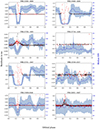 |
Fig. A.2. Same as Fig. A.1 but for PSRs J1555−2908, J1628−3205, J1705−1903, J1719−1438, J1731−1847, J1745+1017, J1959+2048 and J2051−0827. |
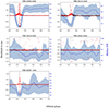 |
Fig. A.3. Same as Fig. A.1 but for PSRs J2055+3829, J2115+5448, J2214+3000, J2234+0944 and J2256−1024. |
Appendix B: Eclipse residuals fits
This appendix refers to Sect. 3.3.
Figure 5 shows an example of eclipse residuals plot for PSR J2256−1024. In Figs. B.1 and B.2 we show the same plot for all eclipsing pulsars in our sample. Best-fit parameters from this analysis are listed in Table 5.
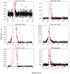 |
Fig. B.1. Same as Fig. 5 but for PSRs J1513−2550, J1555−2908, J1628−3205, J1705−1903, J1731−1847 and J1959+2048. The median-fit function obtained from the analysis presented in Sect. 3.3 is shown in red. The light red zone represents the RMS of the timing residuals for orbital phases ϕ > 06.5, and the dashed vertical lines correspond to the values of Φstart and Φend as inferred from the fit. |
Appendix C: Polarimetric profiles for the 19 spider pulsars
This appendix refers to Sect. 4.
The 1.4 GHz composite profiles shown below were constructed by summing the profiles from individual NUPPI observations conducted after MJD 58800, which are NUPPI observations that were calibrated using the improved polarisation calibration scheme presented in Guillemot et al. (2023). For polarimetric profiles with S/N values larger than 1000, we kept the original number of phase bins of 2048. We reduced the number of phase bins by a factor of 2 for S/N values under 1000, by a factor of 4 under 300, by a factor of 8 under 100 and by a factor of 16 under 30.
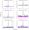 |
Fig. C.1. Polarimetric profiles for PSRs J0023+0923, J0610−2100, J0636+5128, J1124−3653, J1513−2550 and J1544+4937. In each panel, the black line represents the total intensity (Stokes parameter I), the red and purple lines correspond to the Stokes parameters Q and U describing the linear polarisation, and the blue line is the circular polarisation (Stokes parameter V). Pulse profiles were rotated in order for the total intensity maxima to be at phase 0.5. For pulsars with no published RM value we did not correct the Stokes parameters Q and U for Faraday rotation. These pulsars are indicated with an asterisk. |
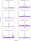 |
Fig. C.2. Same as Fig. C.1 but for PSRs J1555−2908, J1628−3205, J1705−1903, J1719−1438, J1731−1847, J1745+1017, J1959+2048 and J2051−0827. |
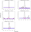 |
Fig. C.3. Same as Fig. C.1 but for PSRs J2055+3829, J2115+5448, J2214+3000, J2234+0944 and J2256−1024. |
Appendix D: Relationship between effective and L1 filling factors
This appendix refers to Table 8.
Roche-lobe geometry is determined by only two parameters: the binary mass ratio q and the binary separation a. The latter acts as a scaling factor. The stellar surface follows an equipotential surface, the largest one being by definition the boundary of the Roche lobe which goes through the L1 Lagrange point.
There is not a unique way of defining the filling factor. The L1 filling factor is defined as
 (D.1)
(D.1)
where rs is the distance from the centre to the surface of the star along the line connecting the two components of the binary system (the intrabinary line), and rL1 is the distance of the Lagrange L1 point. On the other hand the effective-radius filling factor is defined as
 (D.2)
(D.2)
where  and
and  are the volume-averaged radii corresponding to the stellar surface and the Roche lobe, that is the radii of spheres with the same volumes as those enclosed in the stellar surface equipotential and Roche lobe, respectively (Paczynski 1981; Kopal 1978). The effective Roche lobe radius
  can be conveniently calculated using an approximation due to Eggleton (1983).
In this paper we have generated a numerical interpolation of the functions feff(fL1, q), and inversely fL1(feff, q), where q = mp/mc is the mass ratio between the pulsar and its companion. The separation a does not appear since it cancels out in the definition of the filling factors.
To do so, we used the Icarus software (Breton et al. 2012) which is able to compute numerically feff(fL1, q). We computed feff on a grid of 500 mass ratios 1.4 ≤ q ≤ 250, and 100 L1 filling factors 0.1 ≤ fL1 ≤ 1. This grid can then be interpolated (we used basic linear interpolation). In order to invert the relation we used this interpolation coupled with a root finding algorithm to solve feff(fL1, q) = y for fL1(y, q) 4. The difference between the interpolated results and direct calculation with Icarus was not above 0.1% in our validations. The file containing the interpolation grid as well as the python routines converting both ways are available at https://doi.org/10.5281/zenodo.15222623.
In Fig. D.1 we show the difference between the two definitions on our interpolation grid. We see that the difference depends weakly on q as it varies only by ∼10% on the whole range for a fixed fL1. The largest difference between the two definitions is around fL1 ≃ 0.6 where feff ≃ 0.75.
 |
Fig. D.1. Difference between effective radius filling feff factor and L1 filling factor fL1 as a function (fL1, q), where q is the mass ratio. |
All Tables
Astrometric and spin properties of the 19 pulsars constituting our spider pulsar sample.
Published orbital inclinations and Roche-lobe filling factors for the pulsars in our sample.
All Figures
|
Fig. 1. Orbital periods of known spider systems compared against minimum companion masses. In this figure, spider systems are categorised as BW or RB depending on the companion type listed in the ATNF catalogue: Main sequence (MS) stars for RBs or ultra low-mass objects (ULs) in the case of BWs. Some NRT spiders have no information about the companion type in the catalogue; hence, some circles have no cross inside. |
| In the text | |
|
Fig. 2. Time span of the NRT dataset considered in this study. Each dot represents an observation made with the NUPPI backend. |
| In the text | |
|
Fig. 3. Two-dimensional template profile of PSR J0023+0923 as determined using the PulsePortraiture software suite. The sub-components of the main pulse of this pulsar were observed to evolve with frequency, with the first one being brighter than the second at lower frequencies and fainter at the top of the observed bandwidth. When collapsed in frequency, this profile displays two equally bright peaks. |
| In the text | |
|
Fig. 4. Timing residuals and median S/N values as a function of orbital phase for PSR J2055+3829. The TOA residuals are shown as red and black dots, with red dots corresponding to observations with S/N values among the 25% lowest. Error bars, which are much smaller than the vertical scale, are not visible in this figure. The blue curve is the median S/N of the TOAs computed over sliding windows of width 0.1 in orbital phase, and the blue zone shows the median absolute deviation around the median values. The dashed vertical line corresponds to superior conjunction, at orbital phase 0.25. |
| In the text | |
|
Fig. 5. Timing residuals as a function of orbital phase around superior conjunction, indicated with a solid line for PSR J2055+3829. The best-fit function obtained from the analysis presented in Sect. 3.3 is shown in red. The light red zone shows the RMS of the timing residuals for orbital phases ϕ > 0.5, and the dashed vertical lines correspond to the values of Φstart and Φend as inferred from the fit. |
| In the text | |
|
Fig. 6. Linear polarisation fractions and absolute circular polarisation fractions for the 682 pulsars from Wang et al. (2023a). Grey diamonds are slow pulsars, and grey dots represent isolated MSPs or MSPs in non-spider systems (pulsars orbiting white dwarf companions or main sequence stars). Red stars are spiders that are not in the NRT sample, and green stars are the spiders analysed in this article. The values for the latter objects can be found in Table 7. |
| In the text | |
|
Fig. 7. Obscuration duration (Tobsc) against delay duration (Tdelay). The grey zone line is the 1:1 line. An eclipsing pulsar on this line would have no ingress and egress phases. The further a pulsar is from this line, the smaller is the fraction of the eclipse over which the beam is not detectable. Colours and shapes depend on the classifications, as given in Table 6: blue circles correspond to the “abrupt” eclipsers, PSRs J1513−2550, J1555−2908 and J2115+5448, red diamonds are the “progressive” eclipsers, PSRs J1628−3205, J2055+3829 and J2256-1024 and green stars are the “shallow” eclipsers, namely PSRs J1705−1903 and J2051−0827. |
| In the text | |
|
Fig. 8. Ingress/egress duration ratio D and ingress/egress slope ratio S as a function of the Tobsc/Tdelay ratio. This ratio is the fraction of the orbit over which the radio beam of the pulsar is not detectable. Values of S and D can be found in Table 6. Colours and symbols are the same as in Fig. 7. |
| In the text | |
|
Fig. 9. Mass function distributions for the pulsars in our sample. |
| In the text | |
|
Fig. 10. Eclipse parameters as determined from the phenomenological fits made in Sect. 3.3 as a function of mass function values. As in Figs. 7 and 8, we respectively represent ‘abrupt’, ‘progressive’ and ‘shallow’ eclipsers with circles, diamonds, and stars. Crosses represent non-eclipsing systems. |
| In the text | |
|
Fig. 11. Comparison between the results of the phenomenological fits made in Sect. 3.3 and summarised in Table 6 and the published inclinations and Roche-lobe filling factors listed in Table 8. The symbols are the same as in Figs. 7 and 8: circles correspond to the ‘abrupt’ eclipsers, diamonds are the ‘progressive’ eclipsers, and stars are the ‘shallow’ eclipsers. Crosses are for non-eclipsing systems. |
| In the text | |
|
Fig. 12. Equivalent width (top panel) and width at 10% of the maximum (bottom panel) as a function of the mass function. The PSRs J1719−1438 and J1628−3205 are not shown for the reasons stated in Sect. 5.2, and PSR J1124−3653 is also not plotted, as the noise baseline in its pulse profile is higher than 10% of the maximum intensity (see Fig. C.1). |
| In the text | |
|
Fig. A.1. Same as Fig. 4 but for PSRs J0023+0923, J0610−2100, J0636+5128, J1124−3653, J1513−2550 and J1544+4937. We note that in this figure S/N histograms and corresponding axes are shown in blue. TOA residuals are shown as red and black dots. Red dots correspond to observations with S/N values among the 25% lowest. Dashed vertical lines indicate superior conjunction, corresponding to orbital phase 0.25. In some plots the error bars are too small to be apparent. |
| In the text | |
|
Fig. A.2. Same as Fig. A.1 but for PSRs J1555−2908, J1628−3205, J1705−1903, J1719−1438, J1731−1847, J1745+1017, J1959+2048 and J2051−0827. |
| In the text | |
|
Fig. A.3. Same as Fig. A.1 but for PSRs J2055+3829, J2115+5448, J2214+3000, J2234+0944 and J2256−1024. |
| In the text | |
|
Fig. B.1. Same as Fig. 5 but for PSRs J1513−2550, J1555−2908, J1628−3205, J1705−1903, J1731−1847 and J1959+2048. The median-fit function obtained from the analysis presented in Sect. 3.3 is shown in red. The light red zone represents the RMS of the timing residuals for orbital phases ϕ > 06.5, and the dashed vertical lines correspond to the values of Φstart and Φend as inferred from the fit. |
| In the text | |
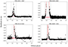 |
Fig. B.2. Same as Fig. B.1 but for PSRs J2051−0827, J2055+3829, J2115+5448, and J2256−1024. |
| In the text | |
|
Fig. C.1. Polarimetric profiles for PSRs J0023+0923, J0610−2100, J0636+5128, J1124−3653, J1513−2550 and J1544+4937. In each panel, the black line represents the total intensity (Stokes parameter I), the red and purple lines correspond to the Stokes parameters Q and U describing the linear polarisation, and the blue line is the circular polarisation (Stokes parameter V). Pulse profiles were rotated in order for the total intensity maxima to be at phase 0.5. For pulsars with no published RM value we did not correct the Stokes parameters Q and U for Faraday rotation. These pulsars are indicated with an asterisk. |
| In the text | |
|
Fig. C.2. Same as Fig. C.1 but for PSRs J1555−2908, J1628−3205, J1705−1903, J1719−1438, J1731−1847, J1745+1017, J1959+2048 and J2051−0827. |
| In the text | |
|
Fig. C.3. Same as Fig. C.1 but for PSRs J2055+3829, J2115+5448, J2214+3000, J2234+0944 and J2256−1024. |
| In the text | |
|
Fig. D.1. Difference between effective radius filling feff factor and L1 filling factor fL1 as a function (fL1, q), where q is the mass ratio. |
| In the text | |
Current usage metrics show cumulative count of Article Views (full-text article views including HTML views, PDF and ePub downloads, according to the available data) and Abstracts Views on Vision4Press platform.
Data correspond to usage on the plateform after 2015. The current usage metrics is available 48-96 hours after online publication and is updated daily on week days.
Initial download of the metrics may take a while.