| Issue |
A&A
Volume 698, June 2025
|
|
|---|---|---|
| Article Number | A289 | |
| Number of page(s) | 12 | |
| Section | Stellar atmospheres | |
| DOI | https://doi.org/10.1051/0004-6361/202453476 | |
| Published online | 25 June 2025 | |
Abundance analysis of benchmark M dwarfs
1
Observational Astrophysics, Department of Physics and Astronomy, Uppsala University,
Box 516,
751 20
Uppsala,
Sweden
2
Thüringer Landessternwarte,
Sternwarte 5,
07778
Tautenburg,
Germany
★ Corresponding author: This email address is being protected from spambots. You need JavaScript enabled to view it.
Received:
17
December
2024
Accepted:
5
May
2025
Abstract
Context. Abundances of M dwarfs, the most numerous stellar type in the Galaxy, can enhance our understanding of planet formation processes. They can also be used to study the chemical evolution of the Galaxy, where α-capture elements play a particularly important role.
Aims. We aim to obtain the abundances of Fe, Ti, and Ca for a small sample of well-known M dwarfs for which interferometric measurements are available. These stars and their abundances are intended to serve as a benchmark for future large-scale spectroscopic studies.
Methods. We analysed spectra obtained with the GIANO-B spectrograph. Turbospectrum and the wrapper TSFitPy were used with MARCS atmospheric models to fit synthetic spectra to the observed spectra. We performed a differential abundance analysis in which we also analysed a solar spectrum using the same method and then subtracted the derived abundances line by line. The median was taken as the final abundance of each element and each star.
Results. Our abundances of Fe, Ti, and Ca mostly agree within the uncertainties with other values from the literature. However, there are few studies to compare with.
Key words: techniques: spectroscopic / stars: abundances / stars: atmospheres / stars: late-type / stars: low-mass
© The Authors 2025
 Open Access article, published by EDP Sciences, under the terms of the Creative Commons Attribution License (https://creativecommons.org/licenses/by/4.0), which permits unrestricted use, distribution, and reproduction in any medium, provided the original work is properly cited.
This article is published in open access under the Subscribe to Open model. This email address is being protected from spambots. You need JavaScript enabled to view it. to support open access publication.
1 Introduction
In recent years, M dwarfs have become favourable targets in the hunt for exoplanets. This is because exoplanets are easier to detect around M dwarfs due to the low mass and faintness of these cool stars, which favours both the radial velocity (RV) and the transit methods. Additionally, the proximity between the star and a potential planet in the habitable zone increases opportunities for characterising the planet using, for example, transit spectroscopy (see, e.g., Luque et al. 2021; Cadieux et al. 2022; Loyd et al. 2024).
These cool and faint stars are the most common type in the Milky Way, accounting for over 70% of the Galactic stars (Henry et al. 2006). The multitude of M dwarfs could make them important in characterising large stellar structures such as clusters. We are, however, still limited by our observational capabilities. M dwarfs could also be important for tracing chemical evolution because of their long expected lifetime and slow evolution. They would be an indicator of the local chemical makeup from when a group was formed. The difficulty would be to estimate the M dwarf age, but this problem could be solved by studying stars in clusters. The multitude of stars also increases the likelihood of finding a habitable exoplanet; it is estimated that each M dwarf has more than two Earth-like exoplanets (Dressing & Charbonneau 2015).
M dwarfs are, however, difficult targets to observe. The cool temperatures in the photosphere of M dwarfs makes it possible for di-atomic and tri-atomic molecules to form, such as TiO, FeH, H2O, and VO (Gray & Corbally 2009). Atomic lines are hidden and blended by these molecular lines. This is especially true in the optical wavelength region, where bands of TiO blend with the atomic lines. In the near-infrared (NIR) we find less strong molecular features and the atomic lines are easier to distinguish, but not without issue. For example, in the H band we find a lot of lines of water molecules; they suppress the continuum, resulting in a pseudo-continuum (Sarmento et al. 2021). There is less water in the J band, but telluric lines are imprinted on the spectra in ground-based observations. One can ignore the telluric lines and use atomic lines in between, observe a telluric standard star, or use software (as explained below) to remove the telluric lines.
Despite these challenges, multiple spectroscopic studies have determined the effective temperatures, metallicities, and surface gravities of M dwarfs. A few examples include Mann et al. (2015), Lindgren et al. (2016); Lindgren & Heiter (2017), Passegger et al. (2018, 2019), Rajpurohit et al. (2018), Sarmento et al. (2021), and Souto et al. (2022). Several of these studies used either calibrations or photometry to obtain the surface gravity because of the degeneracy found between the parameters.
It is important to obtain abundances of stars in general to explore and understand Galactic chemical evolution. In particular, abundances of α-capture elements allow one to determine the relative contributions of the end stages of different types of masses and thereby the nucleosynthetic history of stellar populations within the Milky Way. Studying M dwarfs will also help advance our understanding of planet formation due to the increased number of exoplanets detected. Key elements in this regard are C, S, O, Na, Si, Fe, Mg, Ni, Ca, and Al (in order from most volatile to most refractory; Wang et al. 2019). By determining the abundances of these elements in a host star and accounting for the depletion of volatiles during the formation of rocky planets, the interior compositions and structures of terrestrial exoplanets can be constrained and compared to those of the Earth.
The ratios of the elemental abundances in the star are often assumed to be mirrored in the planet (e.g. Thiabaud et al. 2015; Brinkman et al. 2024), but for some high-density planets indications for differences have been found (e.g. Santerne et al. 2018). These cases can be used to explore the special conditions required to form Mercury-like planets. Few abundance studies of M dwarfs have been published. The following is a sample, with the derived species in parentheses: Woolf & Wallerstein (2005, Fe and Ti), Tsuji & Nakajima (2016, C and O), Abia et al. (2020, Rb, Sr, and Zr), Maldonado et al. (2020, C, O, Na, Mg, Al, Si, Ca, Sc II, Ti, V, Cr, Mn, Co, Ni, and Zn), Shan et al. (2021, V), Souto et al. (2022, C, O, Na, Mg, Al, Si, K, Ca, Cr, Mn, Fe, and Ni), Ishikawa et al. (2022, Na, Mg, Si, K, Ca, Ti, V, Cr, Mn, Fe, and Sr), Melo et al. (2024, Fe, C, O, Na, Mg, Al, Si, K, Ca, Ti, V, and Mn), and Jahandar et al. (2025, Fe, Mg, O, Si, Ca, Ti, Al, Na, C, and K).
When performing abundance analyses it is important to have an accurate effective temperature and surface gravity. In this work we used data obtained with interferometry. With an angular diameter from interferometry and a bolometric flux from photometry, the Stefan-Boltzmann law can be used to obtain model-independent effective temperatures. Using distances from astrometry and empirical mass-luminosity relations, the mass and thereby the surface gravity of the star can be obtained. Past interferometric studies of M dwarfs include Berger et al. (2006), von Braun et al. (2011), Boyajian et al. (2012), von Braun et al. (2014), Kervella et al. (2016), Schaefer et al. (2018), Rabus et al. (2019), Caballero et al. (2022), and Ellis (2022).
Many current and future surveys include M dwarfs in their sample, which means that thousands of M dwarfs need to be accurately characterised. APOGEE (Apache Point Observatory Galaxy Evolution Experiment; Majewski et al. 2017; Jönsson et al. 2020) is primarily targeting red giants but has also observed M dwarfs. Another example is PLATO (PLAnetary Transits and Oscillations of stars; Rauer et al. 2014, 2025), a future space telescope that will use light curves to detect exoplanets. Thousands of M dwarfs are part of the PLATO sample, and spectra from follow-up observations need to be analysed. New methods involving machine learning have been developed to facilitate the analysis of large samples of such stars. Examples include Birky et al. (2020), Passegger et al. (2020, 2022), Rains et al. (2024), and Olander et al. (2025). In some cases the observed spectra of well-known stars are used directly in the training and other times they are used to verify the results. Due to the difficulties discussed above, there has been a lack of well-characterised M dwarfs. We have effective temperatures and surface gravities obtained from interferometry for a set of M dwarfs, but we also need the metallicity and abundances of various elements, especially the α elements. This can be obtained by carefully analysing high-resolution spectra of individual stars, which has been done by the studies referenced above.
In this article, we present an abundance analysis of a sample of M dwarfs with interferometric measurements from Boyajian et al. (2012). In Sect. 2, we introduce our sample and observations. In Sect. 3, we describe our analysis method. In Sect. 4, we present our results, which is followed by a discussion and conclusions in Sect. 5.
2 Sample and observations
The sample of stars presented in this paper consists of well-characterised stars with Teff and log g obtained using interferometry in Boyajian et al. (2012). They obtain Teff by measuring the limb-darkened angular diameter with the CHARA (Center for High Angular Resolution Astronomy) array and using the bolometric flux obtained from HIPPARCOS parallaxes (van Leeuwen 2007) and photometry fitted to spectral templates in the Stefan-Boltzmann law. The surface gravity is obtained using an absolute K-band mass-luminosity relation from Henry & McCarthy (1993). The sample consists of nine stars and includes one binary system. The stars are from spectral type M1 to M4 and in the literature the majority have a subsolar metallicity. The sample can be seen in Table 1 together with the total exposure time and the signal-to-noise ratio (S/N). The S/N is given at 11785 Â, which corresponds to the centre of the part of the spectra used in this article (centre of order 65; see Sect. 2.2). In cases of multiple observations per star (two for GJ 412A, GJ 699, and GJ 725A; four for GJ 436), which were coadded after data reduction during telluric removal (see Sect. 2.3), the S/N is the square root of the sum of the squared S/Ns of each observation.
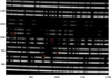 |
Fig. 1 Fragment of a combined spectrum consisting of spectra observed at two nodding positions by GIANO-B. We see replicated spectral lines corresponding to the same spectral orders, the tilt of the slit image, a couple of strong cosmic ray hits, and some detector defects (outlined in red). |
2.1 Observational data
The observations were performed with the GIANO-B spectrograph mounted on the 3.58 m Telescopio Nazionale Galileo on La Palma. GIANO-B is a NIR echelle spectrograph with a resolving power of 50 000 and a wavelength coverage from 9000 to 24 500 Å? (Origlia et al. 2014). Observations were conducted on 25 to 27 May 2019 in visitor mode. The observations were planned with the goal of achieving an S/N of at least 150.
2.2 Data reduction
The focal plane format of GIANO-B represents a challenge for data reduction due to 50 curved spectral orders present in two nodding positions, multiple detector defects, variable tilt of the slit images, etc., as illustrated in Fig. 1, where artefacts are marked in red. We selected to use the REDUCE package (Piskunov & Valenti 2002; Piskunov et al. 2021), which has been successfully tested on several instruments. This includes the ESO VLT CRIRES+ spectrograph1, which has a number of similarities with GIANO-B. After constructing a master flat, tracing spectral orders, and extracting the wavelength calibrations (UNe calibration lamp), we combined the raw frames from the A and B nodding positions and extracted them as one frame, accounting for the slit tilt. The slit orientation was mapped from the UNe frames and then used for the optimal extraction of the science spectra as described in Piskunov et al. (2021). Continuum normalisation in REDUCE requires wavelength overlap between orders, which forced us to restrict the data reduction to the 36 bluest orders (9400-17 000 Å), and here we encountered the biggest challenge in our reduction. The usual initial guess for the continuum fit required for order splicing is the blaze functions, derived from the master flat. These show pronounced fringing with an amplitude of a few percent and a frequency comparable to the width of the spectral lines. To resolve this problem, we first fitted a continuum' to the blaze functions not affected by telluric absorption, then fitted a 2D surface to the upper envelope of the spectral format by associating each blaze point with its position on the detector and interpolating to the orders affected by tellurics. The corrected set of blaze functions was good enough to produce a decent continuum fit for orders 45 to 80 that are used in this article.
Target sample.
2.3 Telluric removal
Telluric lines were removed using an updated version of the software viper2 (Velocity and IP EstimatoR; Zechmeister et al. 2021). The main concept of viper is based on the method described by Butler et al. (1996). The algorithm has been extended by adding a term for the telluric spectrum, which enables its usage for observations taken in the NIR. Using leastsquares fitting, the wavelength solution, blaze, instrument profile and telluric line depths of the observations are modelled simultaneously to account for instrument instabilities and weather changes. Although viper was originally developed for the determination of RVs, it can also be used for pure telluric correction. For the telluric forward modelling viper uses synthetic standard models obtained from Molecfit (Smette et al. 2015) for each molecule in the Earth atmosphere. For details regarding the telluric removal the reader is directed to Köhler & viper Pipeline Team (2024).
We fed viper with pre-normalised spectra and adjusted the settings to obtain the best possible telluric removal. Still we faced problems in the removal of deep tellurics, which cannot be accurately modelled. However, we avoided spectral lines blended with or those that are near strong telluric lines in our analysis. In cases where we have multiple observations for the same star, the spectra were co-added within viper, by using a weighted average of all the telluric-corrected spectra.
3 Method
For the analysis we used Turbospectrum (Alvarez & Plez 1998; Plez 2012; Gerber et al. 2023) together with the wrapper TSFitPy (Gerber et al. 2023; Storm & Bergemann 2023) and MARCS atmospheric models (Gustafsson et al. 2008). It uses the Bergemann et al. (2021) and Magg et al. (2022) solar abundances. TSFitPy fits synthetic spectra generated by Turbospectrum to observed spectra using Nelder-Mead minimisation. In this work we used line-by-line fitting and thereby obtained abundances for each line. To minimise the effects from used models, we performed a differential abundance analysis. We analysed the high resolution solar spectrum provided by Reiners et al. (2016) using the same method as for the M dwarfs. The only differences were that the solar metallicity was always set to zero and we did not alter the Ti and Ca abundances. The other parameters were set to Teff: 5771 K and log g: 4.44 dex3. We then subtracted the solar abundance for each line from the M dwarf abundance for the same line. The solar spectrum was obtained using a Fourier transform spectrograph, and the resolution in the NIR was 106.
For the M dwarf input parameters we used Boyajian et al. (2012) for Teff as well as the radius and mass to calculate log g. The exception is the binary GJ 725A and B, for which we used Mann et al. (2015). There is an inconsistency for the parameters from Boyajian et al. (2012) for the B star. The effective temperature for that star differs significantly from other measurements, which indicates a possible issue with the measured angular diameter. This has been seen for example in Souto et al. (2020) and Olander et al. (2025). For projected equatorial rotational velocity (v sin i) and RV, we used Reiners et al. (2018) and Fouqué et al. (2018). The rotational velocity was fixed throughout the analysis, and set to the upper limit given in the references. Our sample consists of slowly rotating stars and the effect from magnetic broadening should therefore be minimal. We note that our models do not include broadening caused by magnetic fields. The RV is allowed to be adjusted slightly for a better fit. This is done by a second fitting after the abundance; see Storm & Bergemann (2023) for more details. For the results presented in this work the RV rarely shifted by more than 2 km s−1. For input metallicity [Fe/H] we used Mann et al. (2015). TSFitPy calculates the microturbulence Vturb using an empirical relation based on Teff, log g, and [Fe/H]4, which was derived for the data analysis within the Gaia-ESO Public Spectroscopic Survey (M. Bergemann, priv. comm.). We set the macroturbulence as free. The adopted input parameters are given in Table 2.
Stellar parameters used as input data.
3.1 Line data and mask
The abundances determined in this work are based on carefully selected individual atomic lines most suitable for the purpose. However, for a realistic synthetic spectrum calculation including background lines and blends we need information on all transitions, as far as possible, contributing to the spectrum in the observed wavelength range in the stars of interest. At the same time, for an efficient spectrum calculation we want to avoid treating unnecessary transitions. Our line list was thus constructed to include atomic lines relevant for stellar parameters encompassing those of the target stars. For this purpose, we used the VALD database (Piskunov et al. 1995; Ryabchikova et al. 2015; Pakhomov et al. 2019) and its Extract Stellar' mode. The VALD extraction was done on 10 April 2024 using version 3735 of the VALD3 database and software and the default configuration.
We downloaded two line lists between 10 000 and 14 000 Å, one for an effective temperature of 3000 K and a surface gravity of 4.5 dex, and another for Teff=4000 K and log g=5.5 dex. We used the same minimum threshold for the central line depth of 0.0015, a microturbulence of 2 kms−1, and elemental abundances enhanced by 0.5 dex for the extraction of both lists. The lists were subsequently merged by removing duplicates. Detailed information about the individual lines that were analysed along with references can be found in Table A.1. In addition to atomic data, we included molecular data. We used the same molecular line data as Bergemann et al. (2012), and they were obtained from Bertrand Plez in a private communication. We note that for the calculation of the synthetic spectrum in the fitting process all of the atomic transitions extracted from VALD were used (about 1000 in the wavelength range covered by the analysed lines) together with the molecular data.
A line mask was created for each atomic species by visually inspecting an M dwarf spectrum and the solar spectrum. The mask covers the deepest flux point of the observed line and stretches in general from the central wavelength given in the line list to the nearest local maxima to both the left and right. Lines blended with telluric lines and other atomic lines were avoided. The cores of the included lines had to be clearly separated from other line cores, which was assessed on a line by line basis. The software iSpec (Blanco-Cuaresma et al. 2014; Blanco-Cuaresma 2019) was used for producing the line masks. The lines used for each star and each element are listed in Tables A.2 to A.4.
3.2 Metallicity and abundances
We fitted for the abundances of Fe, Ti, and Ca, one at a time in an iterative process as follows. We first fitted for Fe in order to determine the overall metallicity, which was then fixed for the rest of the analysis. We then fitted for Ti and thereafter Ca with the previously derived Ti fixed. We then went back to Ti with Ca fixed and the old Ti as an input parameter. We then analysed Ca again with the last Ti fixed and the previous Ca abundance as an input parameter. This iterative process was done in order to break possible degeneracies and dependences between the abundances. Between each iteration we visually inspected the best fit synthetic spectra and discarded lines that showed a bad fit. This was done by first discarding observed lines containing artefacts. Then we removed lines where the derived abundance was outside of 1 to 2 standard deviations from the median value. Which tolerance was used depended on the number of available lines. If there were few lines, we were more forgiving. The final abundance in each iteration was obtained by taking the median of the abundances derived for the acceptable lines. We obtained the uncertainty in the derived abundances by calculating the median absolute difference (MAD) between the different abundances for each individual line after subtracting the corresponding solar abundances.
4 Results
We present our results in Table 3. For some of the stars our uncertainties are high, this is due to a large spread in derived abundances from the different lines. The lines used in the fitting procedure for each star are indicated in Appendix A. An example of best fitted lines for Fe, Ti, and Ca can be seen in Figs. 2, 3, and 4. In the figures we plot the output synthetic spectra from TSFitPy. We note that for the construction of the figures the observed spectra were only adjusted according to the literature RV and not what the individual lines were fitted for, which is why they do not always line up. In some cases very weak lines in either the solar or M dwarfs spectra were used to increase the number of used lines. The line had to have more than five data points and be clearly visible in comparison to the noise level. An example of this can be seen in Fig. 3 in the last panel were the line in the solar spectrum is really weak. The line is clear when zoomed in more. As can be seen in Figs. 2 to 4, the fit of the lines in both the Sun and in the M dwarf are good. In some cases the line core is not correctly fitted as can be seen for the Ti line at 10 496 Å or at 10 661 Å in Fig. 3 or the Ca line in Fig. 4 at 10 344 Å. This is an issue for some Ti and Ca lines. The cause could be incorrect atomic data or a departure from local thermodynamic equilibrium (LTE; see more in Sect. 5).
In Fig. 5, we compare with the overlapping sample of Ishikawa et al. (2022), Jahandar et al. (2025), Maldonado et al. (2020), and Souto et al. (2022). In the case of [Fe/H], we also include the Mann et al. (2015) sample, which we used for input metallicity. Ishikawa et al. (2022) used spectra from the IRD (InfraRed Doppler) instrument mounted on the Subaru telescope. They generated synthetic spectra using MARCS atmospheric models and line lists from VALD and matched the equivalent widths of the observed spectra with those of the synthetic spectra. Jahandar et al. (2025) used high resolution spectra from CFHT/SPIRou (SPectropolarimètre InfraROUge at the Canada-France-Hawai'i Telescope) and the PHOENIX-ACES grid of synthetic spectra and determined Teff and log g prior to the abundances. Maldonado et al. (2020) used archival HARPS and HARPS-N data. They obtained Teff and metallicity using equivalent widths (msdlines) and log g from mass-radius relations. To get abundances they used a principal component analysis. We grouped Souto et al. (2022) and Melo et al. (2024) together as they used the same method and spectra. They analysed APOGEE spectra using Turbospectrum and MARCS atmospheric models with the BACCHUS wrapper. They obtained Teff, log g, [Fe/H], and oxygen and carbon abundances by using so-called Teff−A(O) and log g-A(O) pairs. They also obtained abundances of various atomic species by fitting individual lines.
In Fig. 5, we compare our results for [Fe/H], [Ti/H], and [Ca/H] with abundances from the literature. Our derived [Fe/H] (left panel) agree within uncertainties with Mann et al. (2015, brown star symbols). One outlier is GJ 809 where we derive 0.221 dex and Mann et al. (2015) −0.06 dex. None of the other studies shown in the figure includes this star. However, Passegger et al. (2019), who used CARMENES6 spectra and PHOENIXACES models, obtain 0.29 dex for the same star when using the combined visual and NIR data. When comparing with the literature values for all of the other stars we mostly agree within uncertainties. The general trend is that our [Fe/H] are lower than the literature values. The spread is largest when comparing with Maldonado et al. (2020). Two outliers are GJ 412A and GJ 699. For GJ 412A we derive −0.45 dex and Maldonado et al. (2020) obtain −0.78 dex. However, Mann et al. (2015) obtain −0.37 dex and Souto et al. (2022) −0.40 dex, which is in better agreement with our results. Our derived [Fe/H] for GJ 699 is significantly lower than three of the studies, −0.58 dex compared with −0.28, −0.34, and −0.40 dex (Maldonado et al. 2020, Jahandar et al. 2025, and Mann et al. 2015). However, Ishikawa et al. (2022) obtain −0.60 dex. Passegger et al. (2019) obtain −0.09 dex when using the combined wavelength regions, and −0.13 and −0.14 dex when using the NIR or the visual alone, respectively. It is clear that this star needs further studies. We note that GJ 699 had the fewest Fe lines used in the fitting (seven).
In the middle panel of Fig. 5, we show the comparison with the literature for [Ti/H]. Our results agree within the uncertainties with those of Melo et al. (2024), Ishikawa et al. (2022), and Jahandar et al. (2025). When comparing with Maldonado et al. (2020) we find a bigger discrepancy, especially at lower [Ti/H]. One outlier is the star GJ 699, for which we derive −0.591 dex and Maldonado et al. (2020) −0.130 dex. Another example is GJ 725A. We note that these two stars show some of the largest differences in [Fe/H] when comparing with Mann et al. (2015). The code used in this work provides the abundance in relation to Fe and it is therefore possible that the discrepancy we see in [Ti/H] is hereditary from [Fe/H]. To determine if this is the case, further study is needed, which is beyond the scope of this paper.
For the [Ca/H] results (right panel of Fig. 5) the spread is large compared with all of the literature values, and our uncertainties are even greater. This is most likely because we had problems fitting the cores of some of the lines as mentioned earlier. One possible explanation for this bad fit could be non-LTE effects, especially in the solar spectrum. We find a clear offset when comparing with Souto et al. (2022) and Melo et al. (2024) where our derived abundances are 0.2 dex lower than those of these authors. The largest spread is found when comparing with Maldonado et al. (2020). GJ 412A is again an outlier when comparing with Maldonado et al. (2020), who derive −0.04 dex compared to our −0.478 dex. Souto et al. (2022) derive an abundance of −0.24 dex.
In Fig. 6, we plot [Ti/Fe] and [Ca/Fe] against [Fe/H] for all the stars in the overlapping sample with the literature studies. For both [Ti/Fe] and [Ca/Fe] we have a large spread, and none of the compared studies line up well with each other. However, the sample here is too small to draw any concrete conclusion regarding trends between the studies.
We have one binary system in the sample, GJ 725 A and B. Binaries are expected to have the same abundances as they were formed from the same molecular cloud. For [Fe/H] there is a difference of approximately 0.15 dex between the stars in the binary, for [Ti/Fe] 0.03 dex, and for [Ca/Fe] 0.1 dex. Maldonado et al. (2020) and Souto et al. (2022) analysed both stars in the binary system. Maldonado et al. (2020) obtain a difference between the A and B components of 0.03 dex for [Fe/H], 0.01 dex for [Ti/Fe], and 0.05 dex for [Ca/Fe]. Souto et al. (2022) obtain a difference of 0.03 dex for [Fe/H] and 0.02 dex for [Ca/Fe] (Ti was not measured for these stars by Souto et al. 2022). The difference we see in abundances between the stars in the binary is an indicator of a high uncertainty in our derived abundances. For the B star our [Fe/H] is close to the Souto et al. (2022) value (−0.33 dex compared to −0.32 dex). It is the A star that differs (−0.48 dex). We note that different spectral lines were used in the fitting of the A star and B star, this can be seen in Table A.2. When we look at the [Ti/H] and [Ca/H] derived for the binary, the difference in abundance between the two binary stars is larger than it is for [Ti/Fe] and [Ca/Fe]. This indicates that it might be the iron abundance for GJ 725A that is problematic. One possible explanation for the much lower [Fe/H] in the A star compared to the B star is the quality of the spectrum. As can be seen in Table 1 the S/N of GJ 725A is lower than that of GJ 725B. A more extended analysis of this binary system is needed.
Abundance ratios with uncertainties.
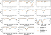 |
Fig. 2 Best-fitted Fe I lines in GJ 436 and the Sun. The observed spectra were only adjusted according to the literature RV and not the RV fit for individual lines. The wavelength range 10 421 Å to 10 425 Å has two Fe lines. In the other panels, the Fe line is in the middle of the plot. |
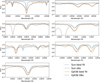 |
Fig. 4 Same as Fig. 2 but for Ca I lines. The wavelength range 12 822 Å to 12 829 Å has two Ca lines. In the other panels, the Ca line is in the middle of the plot. |
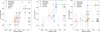 |
Fig. 5 Abundances from this work vs abundances from the literature for stars in overlapping samples. The same star can be found on the same horizontal line with the name of the star to the right in each panel. See the main text for references. |
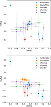 |
Fig. 6 Abundances of Ti and Ca vs Fe for stars in both our sample and other studies from the literature. |
5 Discussion and conclusions
We have successfully used Turbospectrum with MARCS atmospheric models in the wrapper TSFitPy to derive abundances of Fe, Ti, and Ca for a small set of benchmark M dwarfs. We performed a differential abundance analysis with respect to the Sun in order to minimise model dependence. The analysis was performed line by line, and the fitted lines were carefully inspected visually. The fits of the used atomic lines are good, but some of the uncertainties are high. This is partly due to problems with fringing in the observed spectra, but it could also be due to the large gap between spectral types (the Sun and M dwarfs). The fringing caused an incorrect continuum placement for some of the lines, and the resulting abundance for a line could therefore either be too high or too low for those particular lines. We discarded some lines because of issues with the continuum placement. Spectra without fringing would produce a better result with lower uncertainties.
A differential abundance analysis minimises the model dependence of the analysis. However, Gustafsson (1989) discusses that a differential abundance analysis performs better when the analysis is done step-wise if the gap in spectral type is large. The ideal way to analyse an M dwarf would then be to analyse the Sun (G type), a well known K-type star relative to the Sun, and then the M dwarf relative to the K-type star. This would also make it easier to analyse further elements, for example Si. Upon inspection of the spectra in our study, it was found that the available Si lines in the wavelength region we are analysing are strong in the Sun but weak in M dwarfs. The opposite is true for the Ti lines, but in the case of Ti we found a sufficient number of suitable lines to fit. Another way to improve the differential abundance analysis would be to use spectra obtained with the same instrument for all types of stars. This would minimise instrumental effects.
Another possible contributor to the high uncertainties is that we discarded strong lines because of a poor fit between the synthetic and the observed lines. The synthetic lines were either too strong or too weak, and those lines were discarded from the analysis because of derived abundances outside of the accepted range for that star (see Sect. 3). The reason for the bad fit is unknown, but one possible explanation could be incorrect atomic data. We used a generic line list from VALD, which means that no astrophysical corrections of the log gf values were made. Even if the effect of the line list is minimised by the differential abundance analysis, the results would improve with a line list with astrophysically corrected log g f values, which was beyond the scope of this study. Additionally, with a line list optimised for M dwarfs, a differential abundance analysis would not be as necessary.
Our results show a somewhat large spread compared to literature values. However, there is also a spread when comparing the different literature values with each other. This can be clearly seen in Fig. 6, which shows the overlapping sample of stars. We can see that the results from the literature studies differ beyond the uncertainties, which indicates that the uncertainties are underestimated in many studies. The spectroscopic community needs to put more effort into analysing M dwarfs in order to obtain fundamental parameters and abundances. We also need to determine the reasons for the differing results. Doing this would improve our understanding of M dwarfs and the physical conditions inside their atmospheres. Additionally, more abundance analysis studies of a large quantity of M dwarfs are needed in order to draw any conclusions regarding M dwarf abundances in connection to Galactic chemical trends. According to Souto et al. (2022), their Ca abundances agree with the Galactic trend, with [Ca/Fe] increasing towards lower [Fe/H]. The [Ca/Fe] values derived in this work in general follow this trend. This can be seen in the lower panel of Fig. 6, where our values (purple pluses) are higher at lower [Fe/H] and lower at higher [Fe/H]. However, our sample is too small for us to say whether M dwarfs in general follow the Galactic trend of [Ca/Fe].
For some of the lines included in the analysis, but also for some of the discarded lines, there is a small difference in line strength. An example can be seen in the first panel in Fig. 4, where the observed line is stronger than the synthetic line. One reason is incorrect abundances but another is a departure from LTE. This is especially true for the Sun as the conditions in its atmosphere allow for departure from LTE for a significant amount of elements. In Fig. 8 of Lind & Amarsi (2024) we can see that a Ca line in the optical wavelength region is clearly affected by non-LTE effects where the 1D non-LTE line is deeper than the LTE line. We also note that the 3D LTE line is deeper than the 3D non-LTE line, which indicates that the 1D models are missing some physics. To the best of our knowledge, no investigation of non-LTE effects for Ca in M dwarfs has been conducted. M dwarfs are assumed to be in LTE but can be affected by non-LTE, as shown in Olander et al. (2021), where abundance corrections ofup to 0.2 dex are found for K. Non-LTE effects for Ti were investigated in Hauschildt et al. (1997), who found a clear difference between LTE and non-LTE. Nordmeier (2020) find an abundance correction of 0.1 dex between LTE and non-LTE. It is clear that non-LTE needs to be thoroughly investigated for M dwarfs.
In the future we should explore the inclusion of molecular lines when fitting in order to derive the abundances of various elements. Souto et al. (2022) used H2O and OH molecules to find O abundances as well as to derive Teff and log g. Souto et al. (2020) find that using FeH lines does not yield the same [Fe/H] as using atomic Fe lines. They estimate a difference of 0.12 dex between [Fe/H] from Fe I and FeH lines in the H band. In our analysis of the star GJ 699, we found it difficult to derive [Fe/H] as the Fe I lines were weak. In Fig. 2 of Souto et al. (2020), we can see that the stars with lower Teff and [Fe/H] have a better agreement between the [Fe/H] obtained from Fe I lines and that from FeH lines. This means that if we have a first estimate of the iron abundance and the star is cool, we could use FeH lines as well as Fe I lines. This could potentially lower the uncertainty of [Fe/H] in cool, low-metallicity stars such as GJ 699. A more extended investigation is needed to test this. FeH lines could also be used to obtain other parameters such as Teff, as shown in Lindgren et al. (2016) and Lindgren & Heiter (2017).
Acknowledgements
We thank the anonymous referee for valuable comments that helped to improve the manuscript. T.O., U.H., and O.K. acknowledge support from the Swedish National Space Agency (SNSA/Rymdstyrelsen). O.K. also acknowledges funding by the Swedish Research Council (grant agreements nos. 2019-03548 and 2023-03667). Based on observations made with the Italian Tele-scopio Nazionale Galileo (TNG) operated on the island of La Palma by the Fundaciôn Galileo Galilei of the INAF (Istituto Nazionale di Astrofisica) at the Spanish Observatorio del Roque de los Muchachos of the Instituto de Astrofisica de Canarias. This work has made use of the VALD database, operated at Uppsala University and the University of Montpellier. We thank Tanya Ryabchikova for her invaluable work with compiling and assessing atomic data for the VALD database, and Bertrand Plez for providing molecular line lists.
Appendix A Line data and lines fitted for each star
In this appendix we present the atomic data for the spectral lines used in the analysis in Table A.1. We also specify which lines were fitted for each star. Table A.2 shows the Fe lines, Table A.3 shows the Ti lines, and Table A.4 shows the Ca lines. In the last three tables, the leftmost column indicates the rest wavelength in air of each line in Å. There is one column for each star in the analysis where an X' marks if a line was used or not. These tables are referred to in Sect. 3.1.
Atomic data for the spectral lines used in the analysis.
Fitted Fe I lines.
Fitted Ti I lines.
Fitted Ca I lines.
References
- Abia, C., Tabernero, H. M., Korotin, S. A., et al. 2020, A&A, 642, A227 [NASA ADS] [CrossRef] [EDP Sciences] [Google Scholar]
- Alvarez, R., & Plez, B. 1998, A&A, 330, 1109 [NASA ADS] [Google Scholar]
- Bergemann, M., Kudritzki, R.-P., Plez, B., et al. 2012, ApJ, 751, 156 [Google Scholar]
- Bergemann, M., Hoppe, R., Semenova, E., et al. 2021, MNRAS, 508, 2236 [NASA ADS] [CrossRef] [Google Scholar]
- Berger, D. H., Gies, D. R., McAlister, H. A., et al. 2006, ApJ, 644, 475 [NASA ADS] [CrossRef] [Google Scholar]
- Birky, J., Hogg, D. W., Mann, A. W., & Burgasser, A. 2020, ApJ, 892, 31 [Google Scholar]
- Blanco-Cuaresma, S. 2019, MNRAS, 486, 2075 [Google Scholar]
- Blanco-Cuaresma, S., Soubiran, C., Heiter, U., & Jofré, P. 2014, A&A, 569, A111 [CrossRef] [EDP Sciences] [Google Scholar]
- Boyajian, T. S., von Braun, K., van Belle, G., et al. 2012, ApJ, 757, 112 [Google Scholar]
- Brinkman, C. L., Polanski, A. S., Huber, D., et al. 2024, AJ, 168, 281 [Google Scholar]
- Butler, R. P., Marcy, G. W., Williams, E., et al. 1996, PASP, 108, 500 [Google Scholar]
- Caballero, J. A., GonzÅlez-Alvarez, E., Brady, M., et al. 2022, A&A, 665, A120 [NASA ADS] [CrossRef] [EDP Sciences] [Google Scholar]
- Cadieux, C., Doyon, R., Plotnykov, M., et al. 2022, AJ, 164, 96 [NASA ADS] [CrossRef] [Google Scholar]
- Dressing, C. D., & Charbonneau, D. 2015, ApJ, 807, 45 [Google Scholar]
- Ellis, T. 2022, PhD thesis, Louisiana State Univ., USA [Google Scholar]
- Fouqué, P., Moutou, C., Malo, L., et al. 2018, MNRAS, 475, 1960 [Google Scholar]
- Gerber, J. M., Magg, E., Plez, B., et al. 2023, A&A, 669, A43 [NASA ADS] [CrossRef] [EDP Sciences] [Google Scholar]
- Gray, R. O., & Corbally, C. J. 2009, Stellar Spectral Classification (Princeton University Press) [Google Scholar]
- Gustafsson, B. 1989, ARA&A, 27, 701 [Google Scholar]
- Gustafsson, B., Edvardsson, B., Eriksson, K., et al. 2008, A&A, 486, 951 [NASA ADS] [CrossRef] [EDP Sciences] [Google Scholar]
- Hauschildt, P. H., Allard, F., Alexander, D. R., & Baron, E. 1997, ApJ, 488, 428 [NASA ADS] [CrossRef] [Google Scholar]
- Henry, T. J., & McCarthy, Donald W. J. 1993, AJ, 106, 773 [NASA ADS] [CrossRef] [Google Scholar]
- Henry, T. J., Jao, W.-C., Subasavage, J. P., et al. 2006, AJ, 132, 2360 [Google Scholar]
- Ishikawa, H. T., Aoki, W., Hirano, T., et al. 2022, AJ, 163, 72 [NASA ADS] [CrossRef] [Google Scholar]
- Jahandar, F., Doyon, R., Artigau, É., et al. 2025, ApJ, 978, 154 [Google Scholar]
- Jönsson, H., Holtzman, J. A., Allende Prieto, C., et al. 2020, AJ, 160, 120 [Google Scholar]
- Kervella, P., Mérand, A., Ledoux, C., Demory, B. O., & Le Bouquin, J. B. 2016, A&A, 593, A127 [NASA ADS] [CrossRef] [EDP Sciences] [Google Scholar]
- Köhler, J., & viper Pipeline Team 2024, VIPER Manual, ESO, Garching bei München, Germany, https://mzechmeister.github.io/viper_RV_pipeline/ [Google Scholar]
- Kurucz, R. L. 2007, Robert L. Kurucz on-line database of observed and predicted atomic transitions, http://kurucz.harvard.edu/atoms/2000/ [Google Scholar]
- Kurucz, R. L. 2014, Robert L. Kurucz on-line database of observed and predicted atomic transitions, http://kurucz.harvard.edu/atoms/2600/ [Google Scholar]
- Kurucz, R. L. 2016, Robert L. Kurucz on-line database of observed and predicted atomic transitions, http://kurucz.harvard.edu/atoms/2200/ [Google Scholar]
- Lawler, J. E., Guzman, A., Wood, M. P., Sneden, C., & Cowan, J. J. 2013, ApJS, 205, 11 [Google Scholar]
- Lind, K., & Amarsi, A. M. 2024, ARA&A, 62, 475 [NASA ADS] [CrossRef] [Google Scholar]
- Lindgren, S., & Heiter, U. 2017, A&A, 604, A97 [NASA ADS] [CrossRef] [EDP Sciences] [Google Scholar]
- Lindgren, S., Heiter, U., & Seifahrt, A. 2016, A&A, 586, A100 [NASA ADS] [CrossRef] [EDP Sciences] [Google Scholar]
- Loyd, P., Schreyer, E., Owen, J., et al. 2024, in AAS/Division for Extreme Solar Systems Abstracts, 56, 625.22 [Google Scholar]
- Luque, R., Serrano, L. M., Molaverdikhani, K., et al. 2021, A&A, 645, A41 [NASA ADS] [CrossRef] [EDP Sciences] [Google Scholar]
- Magg, E., Bergemann, M., Serenelli, A., et al. 2022, A&A, 661, A140 [NASA ADS] [CrossRef] [EDP Sciences] [Google Scholar]
- Majewski, S. R., Schiavon, R. P., Frinchaboy, P. M., et al. 2017, AJ, 154, 94 [NASA ADS] [CrossRef] [Google Scholar]
- Maldonado, J., Micela, G., Baratella, M., et al. 2020, A&A, 644, A68 [EDP Sciences] [Google Scholar]
- Mann, A. W., Feiden, G. A., Gaidos, E., Boyajian, T., & von Braun, K. 2015, ApJ, 804, 64 [Google Scholar]
- Melo, E., Souto, D., Cunha, K., et al. 2024, ApJ, 973, 90 [Google Scholar]
- Nordmeier, N. 2020, Bachelor thesis, University of Heidelberg, Germany [Google Scholar]
- O'Brian, T. R., Wickliffe, M. E., Lawler, J. E., Whaling, W., & Brault, J. W. 1991, J. Opt. Soc. Am. B Opt. Phys., 8, 1185 [CrossRef] [Google Scholar]
- Olander, T., Heiter, U., & Kochukhov, O. 2021, A&A, 649, A103 [NASA ADS] [CrossRef] [EDP Sciences] [Google Scholar]
- Olander, T., Gent, M. R., Heiter, U., et al. 2025, A&A, 696, A62 [NASA ADS] [CrossRef] [EDP Sciences] [Google Scholar]
- Origlia, L., Oliva, E., Baffa, C., et al. 2014, SPIE Conf. Ser., 9147, 91471E [Google Scholar]
- Pakhomov, Y. V., Ryabchikova, T. A., & Piskunov, N. E. 2019, Astron. Rep., 63, 1010 [NASA ADS] [CrossRef] [Google Scholar]
- Passegger, V. M., Reiners, A., Jeffers, S. V., et al. 2018, A&A, 615, A6 [NASA ADS] [CrossRef] [EDP Sciences] [Google Scholar]
- Passegger, V. M., Schweitzer, A., Shulyak, D., et al. 2019, A&A, 627, A161 [NASA ADS] [CrossRef] [EDP Sciences] [Google Scholar]
- Passegger, V. M., Bello-Garcia, A., Ordieres-Meré, J., et al. 2020, A&A, 642, A22 [NASA ADS] [CrossRef] [EDP Sciences] [Google Scholar]
- Passegger, V. M., Bello-Garcia, A., Ordieres-Meré, J., et al. 2022, A&A, 658, A194 [NASA ADS] [CrossRef] [EDP Sciences] [Google Scholar]
- Piskunov, N. E., & Valenti, J. A. 2002, A&A, 385, 1095 [NASA ADS] [CrossRef] [EDP Sciences] [Google Scholar]
- Piskunov, N. E., Kupka, F., Ryabchikova, T. A., Weiss, W. W., & Jeffery, C. S. 1995, A&AS, 112, 525 [Google Scholar]
- Piskunov, N., Wehrhahn, A., & Marquart, T. 2021, A&A, 646, A32 [NASA ADS] [CrossRef] [EDP Sciences] [Google Scholar]
- Plez, B. 2012, Turbospectrum: Code for spectral synthesis, Astrophysics Source Code Library [record asci:1205.004] [Google Scholar]
- Rabus, M., Lachaume, R., JordÅn, A., et al. 2019, MNRAS, 484, 2674 [Google Scholar]
- Rains, A. D., Nordlander, T., Monty, S., et al. 2024, MNRAS, 529, 3171 [Google Scholar]
- Rajpurohit, A. S., Allard, F., Rajpurohit, S., et al. 2018, A&A, 620, A180 [NASA ADS] [CrossRef] [EDP Sciences] [Google Scholar]
- Rauer, H., Catala, C., Aerts, C., et al. 2014, Exp. Astron., 38, 249 [Google Scholar]
- Rauer, H., Aerts, C., Cabrera, J., et al. 2025, Exp. Astron., 59, 26 [Google Scholar]
- Reiners, A., Mrotzek, N., Lemke, U., Hinrichs, J., & Reinsch, K. 2016, A&A, 587, A65 [NASA ADS] [CrossRef] [EDP Sciences] [Google Scholar]
- Reiners, A., Zechmeister, M., Caballero, J. A., et al. 2018, A&A, 612, A49 [NASA ADS] [CrossRef] [EDP Sciences] [Google Scholar]
- Ryabchikova, T., Piskunov, N., Kurucz, R. L., et al. 2015, Physica Scripta, 90, 054005 [NASA ADS] [CrossRef] [Google Scholar]
- Saloman, E. B. 2012, J. Phys. Chem. Ref. Data, 41, 013101 [NASA ADS] [CrossRef] [Google Scholar]
- Santerne, A., Brugger, B., Armstrong, D. J., et al. 2018, Nat. Astron., 2, 393 [Google Scholar]
- Sarmento, P., Rojas-Ayala, B., Delgado Mena, E., & Blanco-Cuaresma, S. 2021, A&A, 649, A147 [NASA ADS] [CrossRef] [EDP Sciences] [Google Scholar]
- Schaefer, G. H., White, R. J., Baines, E. K., et al. 2018, ApJ, 858, 71 [Google Scholar]
- Shan, Y., Reiners, A., Fabbian, D., et al. 2021, A&A, 654, A118 [NASA ADS] [CrossRef] [EDP Sciences] [Google Scholar]
- Smette, A., Sana, H., Noll, S., et al. 2015, A&A, 576, A77 [NASA ADS] [CrossRef] [EDP Sciences] [Google Scholar]
- Souto, D., Cunha, K., Smith, V. V., et al. 2020, ApJ, 890, 133 [Google Scholar]
- Souto, D., Cunha, K., Smith, V. V., et al. 2022, ApJ, 927, 123 [NASA ADS] [CrossRef] [Google Scholar]
- Storm, N., & Bergemann, M. 2023, MNRAS, 525, 3718 [NASA ADS] [CrossRef] [Google Scholar]
- Thiabaud, A., Marboeuf, U., Alibert, Y., Leya, I., & Mezger, K. 2015, A&A, 580, A30 [NASA ADS] [CrossRef] [EDP Sciences] [Google Scholar]
- Tsuji, T., & Nakajima, T. 2016, PASJ, 68, 13 [Google Scholar]
- van Leeuwen, F. 2007, A&A, 474, 653 [CrossRef] [EDP Sciences] [Google Scholar]
- von Braun, K., Boyajian, T. S., Kane, S. R., et al. 2011, ApJ, 729, L26 [NASA ADS] [CrossRef] [Google Scholar]
- von Braun, K., Boyajian, T. S., van Belle, G. T., et al. 2014, MNRAS, 438, 2413 [CrossRef] [Google Scholar]
- Wang, H. S., Liu, F., Ireland, T. R., et al. 2019, MNRAS, 482, 2222 [NASA ADS] [CrossRef] [Google Scholar]
- Woolf, V. M., & Wallerstein, G. 2005, MNRAS, 356, 963 [NASA ADS] [CrossRef] [Google Scholar]
- Zechmeister, M., Köhler, J., & Chamarthi, S. 2021, viper: Velocity and IP EstimatoR, Astrophysics Source Code Library [record asci:2108.006] [Google Scholar]
CRIRES+ is the upgraded CRyogenic high-resolution InfraRed Echelle Spectrograph at the European Southern Observatory Very Large Telescope.
The units of surface gravity are cm s−2. However, throughout the article, we use the unit dex when specifying values of log g.
Vturb = 1.05 + 2.51 10-4(Teff − t0) + 1.5 10−7(5250 - t0)2 - 0.14(log g - g0) - 0.005(log g - g0)2 + 0.05[Fe/H] + 0.01[Fe/H]2, where t0 = 5500 and g0 = 4.
We note that the central line depth is estimated by the VALD software for extraction, without applying any instrumental or rotational broadening. This information is however not used in the further analysis.
Calar Alto high-Resolution search for M dwarfs with Exoearths with Near-infrared and optical Échelle Spectrographs.
All Tables
All Figures
|
Fig. 1 Fragment of a combined spectrum consisting of spectra observed at two nodding positions by GIANO-B. We see replicated spectral lines corresponding to the same spectral orders, the tilt of the slit image, a couple of strong cosmic ray hits, and some detector defects (outlined in red). |
| In the text | |
|
Fig. 2 Best-fitted Fe I lines in GJ 436 and the Sun. The observed spectra were only adjusted according to the literature RV and not the RV fit for individual lines. The wavelength range 10 421 Å to 10 425 Å has two Fe lines. In the other panels, the Fe line is in the middle of the plot. |
| In the text | |
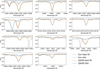 |
Fig. 3 Same as Fig. 2 but for Ti I lines. |
| In the text | |
|
Fig. 4 Same as Fig. 2 but for Ca I lines. The wavelength range 12 822 Å to 12 829 Å has two Ca lines. In the other panels, the Ca line is in the middle of the plot. |
| In the text | |
|
Fig. 5 Abundances from this work vs abundances from the literature for stars in overlapping samples. The same star can be found on the same horizontal line with the name of the star to the right in each panel. See the main text for references. |
| In the text | |
|
Fig. 6 Abundances of Ti and Ca vs Fe for stars in both our sample and other studies from the literature. |
| In the text | |
Current usage metrics show cumulative count of Article Views (full-text article views including HTML views, PDF and ePub downloads, according to the available data) and Abstracts Views on Vision4Press platform.
Data correspond to usage on the plateform after 2015. The current usage metrics is available 48-96 hours after online publication and is updated daily on week days.
Initial download of the metrics may take a while.