| Issue |
A&A
Volume 698, June 2025
|
|
|---|---|---|
| Article Number | A177 | |
| Number of page(s) | 13 | |
| Section | Cosmology (including clusters of galaxies) | |
| DOI | https://doi.org/10.1051/0004-6361/202453446 | |
| Published online | 11 June 2025 | |
Constraints on primordial non-Gaussianity from the cross-correlation of DESI luminous red galaxies and Planck CMB lensing
1
Instituto de Astrofísica de Canarias, C/ Vía Láctea, s/n, E-38205 La Laguna, Tenerife, Spain
2
Department of Physics & Astronomy, University of Rochester, 206 Bausch and Lomb Hall, P.O. Box 270171 Rochester, NY 14627-0171, USA
3
Departamento de Astroísica, Universidad de La Laguna, Avenida Francisco Sánchez, s/n, E-38205 La Laguna, Tenerife, Spain
4
Department of Physics and Astronomy, University of Waterloo, 200 University Ave W, Waterloo, ON N2L 3G1, Canada
5
Perimeter Institute for Theoretical Physics, 31 Caroline St. North, Waterloo, ON N2L 2Y5, Canada
6
Waterloo Centre for Astrophysics, University of Waterloo, 200 University Ave W, Waterloo, ON N2L 3G1, Canada
7
Lawrence Berkeley National Laboratory, 1 Cyclotron Road, Berkeley, CA 94720, USA
8
Department of Physics, Kansas State University, 116 Cardwell Hall, Manhattan, KS 66506, USA
9
Physics Dept., Boston University, 590 Commonwealth Avenue, Boston, MA 02215, USA
10
Dipartimento di Fisica “Aldo Pontremoli”, Università degli Studi di Milano, Via Celoria 16, I-20133 Milano, Italy
11
Department of Physics & Astronomy, University College London, Gower Street, London WC1E 6BT, UK
12
IRFU, CEA, Université Paris-Saclay, F-91191 Gif-sur-Yvette, France
13
Instituto de Física, Universidad Nacional Autónoma de México, Circuito de la Investigación Científica, Ciudad Universitaria, Cd. de México C. P. 04510, México
14
NSF NOIRLab, 950 N. Cherry Ave., Tucson, AZ 85719, USA
15
University of California, Berkeley, 110 Sproul Hall #5800, Berkeley, CA 94720, USA
16
Departamento de Física, Universidad de los Andes, Cra. 1 No. 18A-10, Edificio Ip, CP 111711 Bogotá, Colombia
17
Observatorio Astronómico, Universidad de los Andes, Cra. 1 No. 18A-10, Edificio H, CP 111711 Bogotá, Colombia
18
Institut d’Estudis Espacials de Catalunya (IEEC), c/ Esteve Terradas 1, Edifici RDIT, Campus PMT-UPC, 08860 Castelldefels, Spain
19
Institute of Cosmology and Gravitation, University of Portsmouth, Dennis Sciama Building, Portsmouth PO1 3FX, UK
20
Institute of Space Sciences, ICE-CSIC, Campus UAB, Carrer de Can Magrans s/n, 08913 Bellaterra, Barcelona, Spain
21
Fermi National Accelerator Laboratory, PO Box 500 Batavia, IL 60510, USA
22
Department of Astrophysical Sciences, Princeton University, Princeton, NJ 08544, USA
23
Center for Cosmology and AstroParticle Physics, The Ohio State University, 191 West Woodruff Avenue, Columbus, OH 43210, USA
24
Department of Physics, The Ohio State University, 191 West Woodruff Avenue, Columbus, OH 43210, USA
25
The Ohio State University, Columbus, 43210 OH, USA
26
School of Mathematics and Physics, University of Queensland, Brisbane, QLD 4072, Australia
27
Department of Physics, Southern Methodist University, 3215 Daniel Avenue, Dallas, TX 75275, USA
28
Department of Physics and Astronomy, University of California, Irvine 92697, USA
29
Sorbonne Université, CNRS/IN2P3, Laboratoire de Physique Nucléaire et de Hautes Energies (LPNHE), FR-75005 Paris, France
30
Departament de Física, Serra Húnter, Universitat Autònoma de Barcelona, 08193 Bellaterra, (Barcelona), Spain
31
Institut de Física d’Altes Energies (IFAE), The Barcelona Institute of Science and Technology, Edifici Cn, Campus UAB, 08193 Bellaterra, (Barcelona), Spain
32
Institució Catalana de Recerca i Estudis Avançats, Passeig de Lluís Companys, 23, 08010 Barcelona, Spain
33
Department of Physics and Astronomy, Siena College, 515 Loudon Road, Loudonville, NY 12211, USA
34
Department of Physics & Astronomy and Pittsburgh Particle Physics, Astrophysics, and Cosmology Center (PITT PACC), University of Pittsburgh, 3941 O’Hara Street, Pittsburgh, PA 15260, USA
35
Departamento de Física, DCI-Campus León, Universidad de Guanajuato, Loma del Bosque 103, León, Guanajuato C. P. 37150, Mexico
36
Instituto Avanzado de Cosmología A. C., San Marcos 11 – Atenas 202. Magdalena Contreras, Ciudad de México C. P. 10720, Mexico
37
Instituto de Astrofísica de Andalucía (CSIC), Glorieta de la Astronomía, s/n, E-18008 Granada, Spain
38
Departament de Física, EEBE, Universitat Politècnica de Catalunya, c/Eduard Maristany 10, 08930 Barcelona, Spain
39
Physics Department, Yale University, P.O. Box 208120 New Haven, CT 06511, USA
40
Department of Astronomy, The Ohio State University, 4055 McPherson Laboratory, 140 W 18th Avenue, Columbus, OH 43210, USA
41
Department of Physics and Astronomy, Sejong University, 209 Neungdong-ro, Gwangjin-gu, Seoul 05006, Republic of Korea
42
CIEMAT, Avenida Complutense 40, E-28040 Madrid, Spain
43
University of Michigan, 500 S. State Street, Ann Arbor, MI 48109, USA
44
Department of Physics, University of California, Berkeley, 366 LeConte Hall MC 7300, Berkeley, CA 94720-7300, USA
⋆ Corresponding author: This email address is being protected from spambots. You need JavaScript enabled to view it.
Received:
14
December
2024
Accepted:
14
April
2025
Abstract
Aims. We use the angular cross-correlation between a luminous red galaxy (LRG) sample from the Dark Energy Spectroscopic Instrument (DESI) Legacy Survey data release DR9 and the Planck cosmic microwave background (CMB) lensing maps to constrain the local primordial non-Gaussianity parameter, fNL, using the scale-dependent galaxy bias effect. The galaxy sample covers approximately 40% of the sky, contains galaxies up to redshift z ∼ 1.4, and is calibrated with the LRG spectra that have been observed for DESI Year 1 (Y1).
Methods. We apply a nonlinear imaging systematics treatment based on neural networks to remove observational effects that could potentially bias the fNL measurement. Our measurement is performed without blinding, but the full analysis pipeline is tested with simulations including systematics.
Results. Using the two-point angular cross-correlation between LRG and CMB lensing only, we find fNL = 39−38+40 at the 68% confidence level, and our result is robust in terms of systematics and cosmological assumptions. If we combine this information with the autocorrelation of LRG, applying a scale cut to limit the impact of systematics, we find fNL = 24−21+20 at the 68% confidence level. Our results motivate the use of CMB lensing cross-correlations to measure fNL with future datasets, given its stability in terms of observational systematics compared to the angular autocorrelation. Furthermore, performing accurate systematics mitigation is crucially important in order to achieve competitive constraints on fNL from CMB lensing cross-correlation in combination with the tracers’ autocorrelation.
Key words: cosmic background radiation / cosmology: observations / early Universe / large-scale structure of Universe / inflation
© The Authors 2025
 Open Access article, published by EDP Sciences, under the terms of the Creative Commons Attribution License (https://creativecommons.org/licenses/by/4.0), which permits unrestricted use, distribution, and reproduction in any medium, provided the original work is properly cited.
This article is published in open access under the Subscribe to Open model. This email address is being protected from spambots. You need JavaScript enabled to view it. to support open access publication.
1. Introduction
Cosmic inflation was proposed as a theory in the early 1980s (Guth 1981; Starobinsky 1980). The inflation framework was initially formulated to solve big bang problems such as the horizon, flatness, and magnetic monopole problems; however, inflation is also able to explain the formation of primordial density perturbations (Starobinsky 1982; Guth & Pi 1985; Bardeen et al. 1983). Inflation is defined as a phase in which the Universe is expanding exponentially, driven by a scalar field, ϕ. Several models of inflation have been proposed in the literature (see e.g., Langlois 2010; Vazquez Gonzalez et al. 2020 for a review). The model of inflation and its predictions are defined by choosing the form of the potential, V(ϕ). The simplest inflationary models predict Gaussian initial conditions; however, alternative inflationary models predict different levels of non-Gaussianity in the primordial density perturbations (Chen 2010; Takahashi 2014). The level of non-Gaussianity has usually been characterized in the literature with the fNL non-Gaussianity parameter, such that detecting fNL ≠ 0 is a signature of having non-Gaussian initial conditions.
The tightest constraint on fNL is currently provided by the measurements from the cosmic microwave background (CMB) bispectrum. Using Planck 2018 data, a value fNL = −0.9 ± 5.1 at the 68% confidence level is found (Planck Collaboration IX 2020). However, Dalal et al. (2008) first noticed that local non-Gaussian initial conditions lead to a characteristic scale-dependent signature in the galaxy bias, following a 1/k2 scale-dependence in the ratio between the total matter to observed density of galaxies. During the last decade, many works have performed measurements from the large-scale structure using the scale-dependent bias effect (Ross et al. 2012; Castorina et al. 2019; Mueller et al. 2022; Cabass et al. 2022; D’Amico et al. 2025, among others). In the last years, some measurements from large scale structure (LSS) using the scale-dependent galaxy bias have been achieved using the quasars from the data release DR16 of the Extended Baryon Oscillation Spectroscopic Survey (eBOSS): Mueller et al. (2022) measure fNL = −12 ± 21 and Cagliari et al. (2024) obtain −4 < fNL < 27 using different methodologies. More recently, Chaussidon et al. (2024) have improved this constraint to  using the 3D power spectrum of the Dark Energy Spectroscopic Instrument (DESI) data release DR1 galaxies and quasars. This is a challenging measurement because it requires very accurate control of the largest scales where the scale-dependent bias effect due to fNL arises. Further, it is also important to mention that, when performing fNL measurements from LSS, unless using certain assumptions we actually measure the product of fNL times an unknown bias (see Sect. 2.1 for more details).
DESI (Levi et al. 2013) is a spectroscopic survey that is currently being carried out from the 4 m Mayall telescope at Kitt Peak National Observatory (Arizona, USA). Its unique design with 5000 fibers with robotic positioners allows it to take thousands of spectra in a single exposure (DESI Collaboration 2016a, 2022; Silber et al. 2023; Miller et al. 2024; Guy et al. 2023; Schlafly et al. 2023). Theoretical forecasts (DESI Collaboration 2016b) expect that the full five-year survey will have the ability to achieve a sensitivity σ(fNL)∼5, similar to the best current CMB bispectrum constraint, if there is a good control of systematic effects. Before the first spectroscopic data releases (DESI Collaboration 2024a, 2024b) and science results (DESI Collaboration 2025a, 2025b, 2025c; DESI Collaboration 2024c, 2024d) came out, a full imaging survey was performed in order to select the spectroscopic targets. This targeting survey is called the DESI Legacy Survey (Dey et al. 2019) and covers a broad area (≳20 000 deg2), making it useful for measuring fNL using the scale-dependent galaxy bias. Two previous works have already used the DESI Legacy Survey information to put a constraint on fNL: Rezaie et al. (2024) used the angular power spectra of the louminous red galaxy (LRG) targets, and Krolewski et al. (2024) used the cross-correlation between quasar targets and the Planck CMB lensing.
CMB lensing describes the remapping of the CMB anisotropies due to gravitational lensing by structures along the line of slight. The CMB lensing potential can be easily measured from the observations of the lensed sky (Hu & Okamoto 2002) and was first detected by Smith et al. (2007). Since it contains information about the large-scale structure geometry, its cross-correlation with galaxy tracers can be useful to constrain cosmology. Although CMB lensing and galaxy tracers probe the same structures, they are affected by different systematics, making the cross-correlation between the two a powerful additional tool for measurements into the systematics-dominated regime. Several authors have stressed, using theoretical forecasts, the capabilities of the cross-correlation between CMB lensing and galaxy matter tracers to better constrain fNL (e.g., Jeong et al. 2009; Schmittfull & Seljak 2018; Giusarma et al. 2018; Ballardini et al. 2019; Bermejo-Climent et al. 2021; Perna et al. 2023). More recently, Krolewski et al. (2024) find  using the cross-correlation between Planck lensing and DESI quasar targets. Additionally, recent data analysis works have been performed to constrain other cosmological parameters such as the amplitude of matter density fluctuations, commonly parametrized in terms of σ8 (the RMS density contrast smoothed on a scale of 8 h/Mpc), and matter density, Ωm, using CMB cross-correlations with the DESI Legacy Survey (e.g., White et al. 2022a, Sailer et al. 2024; Kim et al. 2024).
In this paper, we intend to extend the analysis done by Rezaie et al. (2024) with the DESI LRG sample to the inclusion of the CMB lensing cross-correlation as additional information and an additional technique to limit the impact of observational systematics. In Rezaie et al. (2024), an extensive and detailed effort was made to remove observational systematics that could bias the primordial non-Gaussianity (PNG) measurement. Nonetheless, they conclude that their results motivate further studies of PNG with samples less sensitive to systematics like LRG spectroscopic data. Here, our aim is to explore the ability of CMB lensing – LRG cross-correlation to constrain fNL and its stability in terms of systematics, alone and in combination with the LRG autocorrelation.
In Sect. 2 we review the theoretical framework for the imprints of fNL in a scale-dependent galaxy bias and for the cosmological observables we study in the angular domain. In Sect. 3 we present the DESI LRG and Planck lensing datasets used for our analysis. In Sect. 4 we describe the methodology followed for treating our datasets, including a systematics mitigation, computation of observables, and parameter inference pipeline. In Sect. 5 we discuss a validation of our analysis pipeline with mock LRG and CMB lensing fields. In Sect. 6 we present our results for the measurement of PNG and some robustness tests, and in Sect. 7 we summarize our conclusions.
2. Theory
In this section we first provide a description of the physical model that originates a scale-dependent galaxy bias due to a local PNG. We then describe the cosmological observables in the 2D harmonic space involved in our analysis.
2.1. Primordial non-Gaussianity and scale-dependent bias
If we assume a type of non-Gaussianity that depends only on the local value of the potential, the parametrization of the primordial potential can be written as (Komatsu & Spergel 2001)
 (1)
(1)
where fNL is the parameter that describes the amplitude of the quadratic non-Gaussian term and ϕ is a random Gaussian field. We studied fNL through its impact on the scale-dependent galaxy bias, as introduced in Dalal et al. (2008). If we assume the so-called universality relation (Slosar et al. 2008), the contribution to the galaxy bias is expressed as
 (2)
(2)
where δcrit = 1.686 is the threshold overdensity for spherical collapse, bg is the galaxy bias as a function of the redshift z, p is a parameter characterizing the tracers’ response to PNG, assumed as p ≃ 1 for the case of LRG, and α(k) is the relation between potential and density field, such that δ(k) = α(k)Φ(k). The value of α(k) is given by
 (3)
(3)
where T(k) is the transfer function, D(z) is the growth factor (normalized to be 1 at z = 0), Ωm the matter density, and the factor g(∞)/g(0)≃1.3 accounts for the different normalizations of D(z) in the CMB and LSS literature. This definition of fNL is therefore the so-called CMB convention. Other authors (e.g., Carbone et al. 2008; Afshordi & Tolley 2008; Grossi et al. 2009) refer to the use of the ‘LSS convention’, where the g(∞)/g(0) factor is absorbed into the definition of fNL, such that  . Throughout this paper we use p = 1 as a baseline; however, many works based on dark-matter-only simulations (e.g., Adame et al. 2024) find significant deviations from p = 1. In this direction, other authors (e.g., Barreira 2020, 2022) have stressed that we can only constrain the product bϕfNL through the scale-dependent bias effect, where bϕ is a parameter usually defined as bϕ = 2δcrit(bg − p), in order to account for the uncertainties on p.
2.2. Cosmological observables
In this work, we focus on the angular power spectrum of the galaxy – CMB lensing cross-correlation, CℓκG, as well as the galaxy autocorrelation, CℓGG. The angular power spectrum can be calculated as
 (4)
(4)
where 𝒫(k) ≡ k3P(k)/(2π2) is the dimensionless primordial power spectrum and IℓX(k) is the kernel for the X field for unit of primordial power spectrum.
All the weak lensing quantities can be defined from the lensing potential
 (5)
(5)
where  is the gravitational potential. The comoving distance is
 (6)
(6)
The observable two-dimensional lensing potential, averaged over background sources with a redshift distribution Wb(χ), is given by
 (7)
(7)
where qb(χ) is the lensing efficiency for a given background distribution, Wb, defined as
 (8)
(8)
By expanding the gravitational potential in Fourier space and using the plane-wave expansion, we can define the lensing potential kernel as
 (9)
(9)
where Ωm is the present-day matter density, a(χ) is the scale factor, H0 is the Hubble constant, δ(k, χ) is the comoving-gauge linear matter density perturbation, and jℓ the spherical Bessel functions. In case of CMB lensing, the source distribution can be approximated by WCMB(χ) ≃ δD(χ−χ*) and the lensing efficiency by
 (10)
(10)
where χ* is the comoving distance at the surface of last scattering, and Eq. (9) reduces to
 (11)
(11)
Finally, the convergence κ = ∇2ϕ/2 can be expanded in spherical harmonics as
 (12)
(12)
We then relate the two kernels by
 (13)
(13)
The two-dimensional integrated window function for the galaxy number counts is
 (14)
(14)
where Δℓ(k, χ) is the observed number count and W(χ) is a window function given by the redshift distribution of galaxies. At first order, the most important contribution to Δℓ(k, χ) is given by the synchronous gauge source counts Fourier transformed and expanded into multipoles, Δℓs(k, χ). We assumed that Δℓs(k, χ) is related to the underlying matter density field through a scale- and redshift-dependent galaxy bias, bg, as
 (15)
(15)
where bg(k, χ) is given by the sum of a linear bias, which is not scale dependent, plus the scale-dependent contribution given by Eq. (2). We also considered nonlinear contributions to the power spectrum using halofit (Takahashi et al. 2012). In this paper, we also consider two important contributions to the total observed number counts: the effects of redshift space dirtortions (RSD) and lensing magnification (see Fig. 4 for more details). The RSD term is given by
 (16)
(16)
where vk is the velocity of the sources and ℋ is the conformal Hubble parameter. The lensing convergence contribution is given by
 (17)
(17)
where s is the magnification bias that accounts for the fact that observed galaxies are magnified by gravitational lensing. We note that there are other contributions from general relativity to the number counts, but we consider them of second order since the most important contribution to CℓκG is the lensing magnification (see e.g., Appendix A of Bermejo-Climent et al. 2021).
In practice, to numerically evaluate the observables described in this section, we used the Limber approximation (Limber 1953) for ℓ ≥ 100 and computed the full quantities for ℓ < 100, following the implementation in the CAMBSOURCES module (Challinor & Lewis 2011). This was done in order to improve the computational efficiency while having a good estimation of the theory model at the lower multipoles, where the Limber approximation is less accurate. More details on the code used for the computation of theoretical observables can be found in Sect. 4.3.
3. Datasets
We describe in this section the datasets involved in our analysis. The two main ingredients were an LRG photometric catalog from the DR9 Legacy Survey (Zhou et al. 2023a) and the Planck PR4 public CMB lensing maps (Carron et al. 2022). We also used an LRG spectroscopic sample from the DESI Survey Validation data to calibrate the redshift distribution of the photometric DESI LRGs.
3.1. Luminous red galaxies
Our galaxy sample consisted of an LRG catalog obtained from the DESI Imaging Legacy Surveys1 DR9 (Dey et al. 2019). These surveys were a combination of three projects: the Dark Energy Camera Legacy Survey using the Blanco 4m telescope in Chile (DECaLS, Flaugher et al. 2015), the Beijing-Arizona Sky Survey using the Bok telescope at Kitt Peak (BASS, Zou et al. 2017), and the Mayall z-band Legacy Survey (MzLS, Dey et al. 2019) using the Mayall telescope at Kitt Peak. BASS and MzLS observed the same region in the north galactic cap (NGC), while DECaLS observed in both the NGC and south galactic cap (SGC). The combination of the three projects covered ∼19 000 deg2 in the sky to select the spectroscopic targets that are currently being observed with DESI.
We calibrated the redshift distribution, dN/dz, of the sample using the actual LRG spectra measured with the DESI Survey Validation (DESI Collaboration 2024a, 2024b). In Fig. 1 we show the redshift distribution of the sample as obtained from the LRG spectra. These spectra are not available for declinations lower than −30°, hence we removed the Dec < − 30° region from the photometric LRG footprint. Zhou et al. (2023a) also describe the presence of a photometric zero-point systematic effect at low declinations. The resulting final sample contains around 9 million galaxies covering a ∼16 000 deg2 area. Then, we applied to the LRG catalog the mask designed by Zhou et al. (2023b) to reduce contamination from effects such as stars and foregrounds. We pixelized the LRG catalog, converting it into a HEALPix (Gorski et al. 2005) galaxy counts map at Nside = 256. This map is corrected for the pixel incompleteness effect, which accounts for area losses on scales smaller than a Nside = 256 HEALpix pixel, such as cutouts around bright stars. Lastly, the galaxy counts map can be easily converted into an overdensity field by normalizing and subtracting the mean density. We show the LRG overdensity field in Fig. 2.
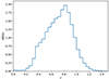 |
Fig. 1. Normalized redshift distribution of the LRG sample, directly measured using the spectroscopic redshifts from DESI Y1 data. |
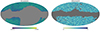 |
Fig. 2. Left panel: LRG overdensity field in galactic coordinates, after applying the δ < −30° cut. Right panel: CMB lensing field in galactic coordinates, obtained from the Planck PR4 maps. |
We note that, since this sample contains photometric redshifts, one could design optimal weights in order to enhance the fNL signal by emphasizing the higher redshift part of the LRG sample. We do not perform this kind of analysis here since we consider it to be beyond the scope of this paper.
3.2. CMB lensing
The other ingredient in our analysis was the Planck CMB lensing potential map. We used the Planck PR4 reconstruction of the CMB lensing potential (Carron et al. 2022), which was obtained from the Planck NPIPE temperature and polarization maps (Akrami et al. 2020). In particular, we used the minimum-variance estimate from temperature and polarization, after mean-field subtraction of the lensing convergence. This latest release of CMB lensing maps improves the noise with respect to the previous Planck PR3 maps (Planck Collaboration VI 2020); in particular, the large-scale noise is lower and the mean-field is better understood thanks to the larger number of simulations. The maps and the mask are publicly available2. We show the CMB lensing field in Fig. 2.
We note that the CMB lensing map does not have the Monte Carlo multiplicative correction applied in Carron et al. (2022). We computed this correction based on simulations as in Krolewski et al. (2024), using mode-decoupled pseudo-Cℓ, and applied the result as a multiplicative factor to the measured cross-correlation angular power spectra, CℓκG. This correction cannot be applied in a general way, since it depends on the footprint mask for each tracer involved in the analysis, due to local variations of the normalization. The order of this correction is generally ≲5%, but it becomes larger (∼10–12%) for the largest scales, having thus a non-negligible impact on the fNL measurements.
4. Analysis pipeline
In this section, we describe the pipeline implemented to analyze the LRG and CMB lensing HEALPix maps. The first step was to apply an imaging systematics mitigation code to the LRG maps. This mitigation treatment operates at the map level and returns a series of systematic weights for each pixel that are applied to the raw LRG maps. Then, we computed the angular power spectrum, Cℓ, of the LRGs, their cross-correlation with the Planck lensing, and the covariance matrices. The final step was to perform a Monte Carlo Markov chain (MCMC) based parameter inference to constrain fNL.
4.1. Imaging systematics mitigation
Imaging systematics due to effects such as extinction, stellar contamination, or changes in the observational conditions usually generate an excess of power at large scales (low multipoles), where the fNL signal arises. Thus, an efficient imaging systematics treatment is key for measuring an unbiased fNL. Rezaie et al. (2020) present a neural network approach for systematics mitigation as a way to model the relation between the observed galaxy density fields and the imaging systematics templates. This pipeline is implemented in the SYSnet code, which is publicly available3. In Rezaie et al. (2024), a detailed study of the performance of SYSnet was done using this LRG sample, with the aim of measuring fNL from the CℓGG autospectra. A different number of approaches were explored, given that SYSnet can return different results depending on the selection of features (imaging systematics template maps) used to perform the regression.
In this work, we used a mitigation recipe optimized for measurements from the cross-correlation between the DESI LRG and Planck lensing, CℓκG. At first order, the cross-correlation itself as a technique would be enough to remove the effects of the systematics if we assumed there were no correlated systematics between the CMB lensing and LRG maps. However, there could still be potential correlated systematics due to galactic foregrounds that affect both probes. Furthermore, the noise in CℓGG contributes to the CℓκG covariance matrix: systematics affecting the CℓGG power spectrum would also lead to an increase in the CℓκG covariance, and as a result, larger uncertainties on fNL. At the same time, a very aggressive mitigation recipe could remove real clustering signal and overfit the CℓκG power spectrum, biasing the fNL measurements toward lower values. For this reason, in order to find a compromise between removing the excess of power spectrum due to systematics for CℓGG and avoiding a strong overfit of CℓκG, we selected the “nonlinear three maps” recipe from Rezaie et al. (2024). This choice is the most conservative one among the recipes applied in Rezaie et al. (2024) with the SYSnet code, and relies on selecting three features or systematics templates for the regression: extinction, galactic depth in the z-band, and point spread function (PSF) size in the r-band. We refer the reader to Rezaie et al. (2024) for more details on the different possibilities of feature selection. In Sect. 5 we also show that this prescription provides unbiased measurements of the angular power spectrum on contaminated mocks.
4.2. Angular power spectra and covariance matrix
In order to estimate the angular power spectra of the LRG autocorrelation and their cross-correlation with the Planck lensing, we used the pseudo-Cℓ approach implemented in the publicly available NaMaster code by Alonso et al. (2019). The pseudo-Cℓ of a pair of fields can be defined as
 (18)
(18)
where X and Y are the observed fields. Then, the difference between the true and measured Cℓ due to the effects of the mask is accounted for through the mode-coupling matrix Mℓℓ′ as
 (19)
(19)
In our case, we directly applied a completeness mask to the observed LRG density, so we just deconvolved the binary footprint mask. In practice, the inversion of the Mℓℓ′ matrix is done using the MASTER algorithm (Hivon et al. 2002), which requires a discrete binning of the angular power spectrum. We used the implementation in the compute_full_master function from the NaMaster code to calculate CℓκG and CℓGG. We binned the theory curves using the same bandpower window functions.
As scale cuts, for CℓκGwe adopted ℓmin = 2 and ℓmax = 300, and we binned the power spectra using Δℓ = 5 for ℓ < 100 and Δℓ = 50 for ℓ > 100. The reason for using this scheme was to obtain a good sampling of the angular power spectra at large scales where the fNL signal arises and ℓmax = 300 is safe enough to minimize the limitations of modeling the nonlinear scales, which could potentially affect the measurement of the linear bias. We checked, with mock fields, that the results are stable with both Nside and ℓmax (see Sect. 5 for more details on the mocks). For CℓGG, we implemented the same multipole binning scheme, but we dropped the first multipole bin of the analysis and set ℓmin = 7. The motivation for this choice was to use a scale cut for CℓGG that limits the impact of remaining systematics according to the mitigation pipeline tests on mocks (see Sect. 5 for more details).
We show in Fig. 3 the measured power spectra of the LRG autocorrelation, CℓGG, and its cross-correlation with the Planck lensing, CℓκG, obtained using uncorrected (raw) LRG maps and LRG maps mitigated with the neural network pipeline. For the covariance matrices, we used the analytic gaussian_covariance function in NaMaster (García-García et al. 2019) to compute the full Gaussian covariance for a masked field. We accounted for the potential extra power in CℓGG due to systematics by smoothing the measured angular power spectra from the data and using this as input for the covariance matrix computation. As a test, we also computed the covariance using mock fields, obtaining compatible results. More details of the mock fields used can be found in Sect. 5. We show in Fig. 5 the computed joint correlation matrix for CℓGG and CℓκG.
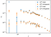 |
Fig. 3. Angular power spectra of the LRG autocorrelation, CℓGG, and CMB lensing – LRG cross-correlation, CℓκG, obtained from the raw (uncorrected) data and after applying the systematics mitigation pipeline to the LRG maps. |
4.3. Likelihood and parameter inference
We defined the likelihood, ℒ, as
 (20)
(20)
where Cℓobs are the elements of the data vector,  is the theoretical model of the angular power spectrum for a given set of parameters, θ, and Cov−1 is the inverse of the covariance matrix.
Our theoretical model is based on the Code for Anisotropies in the Microwave Background, CAMB (Lewis & Challinor 2011). This code is publicly available4 and allows the computation of the angular power spectra of the CMB fields and also galaxy fields, given a window function determined by the galaxy bias, bg, and the redshift distribution, dN/dz. We slightly modified the code to include the scale dependence of the galaxy bias induced by fNL. The dN/dz was directly measured using the DESI LRG spectra from the Survey Validation (DESI Collaboration 2024a, 2024b). The rest of the fiducial cosmological parameters in CAMB are fixed to the Planck 2018 best-fit estimates (Planck Collaboration VI 2020), except for σ8, which we set to a fiducial value σ8 = 0.77 to be in agreement with the measurements from the cross-correlation between the Atacama Cosmology Telescope (ACT) lensing and this LRG sample (Sailer et al. 2024; Kim et al. 2024).
In the computation of the theoretical angular power spectra with the CAMB code, we included the lensing magnification contribution to the galaxy number counts. This effect accounts for the fact that the light from distant galaxies is affected by structures along the line of sight, resulting in an increased flux. The lensing magnification contribution to the angular power spectra could be included in CAMB once we specified the magnification bias, s, as an input parameter. This parameter depends on the galaxy tracer, and for this LRG sample we fixed the magnification bias value to s = 0.999, as determined in Kitanidis & White (2021). More recent measurements using this sample split into four redshift bins (White 2022b; Zhou et al. 2023a) find compatible results within the uncertainty for the various redshift bins; hence, we considered as safe enough the assumption of a z-independent value for s. In Fig. 4 we show the relative importance of the lensing magnification contribution to the CℓGG and CℓκG theoretical angular power spectra, which can be expressed as  . This was calculated with CAMB by adding or neglecting the contribution to the galaxy number counts described in Eq. (17). The impact at the lowest multipoles can reach up to ∼15% for the LRG autocorrelation and ∼35% for the LRG – CMB lensing cross-correlation; hence, this effect is not negligible in our theoretical model for this tracer.
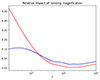 |
Fig. 4. Relative impact of the lensing magnification contributions for the CℓGG (blue line) and CℓκG (red line) theoretical angular power spectra obtained with CAMB. |
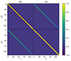 |
Fig. 5. Correlation matrix as obtained from the joint covariance matrix for CℓGG and CℓκG computed with the NaMaster code. |
To compute the constraints on the cosmological parameters, we implemented our likelihood using the MCMC sampler emcee5 (Foreman-Mackey et al. 2013). Our analysis includes fNL and the galaxy bias at z = 0, b0, as the two main cosmological parameters of interest to constrain. We assumed a fiducial redshift evolution of the galaxy bias following
 (21)
(21)
where D(z) is the growth factor normalized to be 1 at z = 0. This choice was motivated by the analysis in Zhou et al. (2021), where a bias evolution compatible with b(z)≃1.5/D(z) was found for the DESI LRG targets. For CℓGG, we also considered the shot noise, Nshot, as a nuisance parameter. We did not impose any prior knowledge on the b0 and Nshot parameters, but restricted their sampling to positive values to avoid nonphysical results.
5. Validation with mocks
Before applying the analysis pipeline described in the previous section to the real LRG and CMB lensing data, we tested it with mock Gaussian fields that simulated the DESI Legacy Survey LRG sample and the Planck lensing observations. For the LRG, we used a sample of 100 Gaussian fields for fNL = 0, 50, and −50. For the CMB lensing, we used a set of 100 correlated maps. These correlated fields were generated using the healpy6 Python package.
We first used CAMB to compute the theoretical angular power spectra CℓGG, CℓκG, and Cℓκκ, given the redshift window function dN/dz obtained from the spectroscopic LRG redshift distribution and the different values of fNL. The galaxy bias parameter at z = 0 was set to a fiducial value of b0 = 1.5, based on Zhou et al. (2021). The fiducial cosmological parameters were set according to the Planck 2018 measurements (Planck Collaboration VI 2020).
The theoretical angular power spectra were used as input for the healpy.synfast function. Following the recipe in Giannantonio et al. (2008), Serra et al. (2014) for simulating correlated fields, we first built a CMB lensing map with a given seed and power spectrum, Cℓκκ. Then, we generated another map with the same seed and power spectrum, (CℓκG)2/Cℓκκ, and we added to this last map another component with a different seed and power spectrum, CℓGG − (CℓκG)2/Cℓκκ. These maps will have amplitudes given by
 (22)
(22)
where ξ1 and ξ2 are random amplitudes, that is, complex numbers with zero mean and unity variance. It is easy to show that
 (23)
(23)
The output products are a subsample of 100 mock CMB lensing fields and 100 correlated LRG overdensity fields, with Nside = 256 for each value of fNL. Lastly, we applied to the mocks the same masks we used for the LRG and CMB lensing data.
In order to test the performance of the systematics mitigation pipeline, we contaminated the LRG maps. For this purpose, after generating the mock LRG and CMB lensing fields, we used the regressis7 code (Chaussidon et al. 2021). From the LRG density fields, we simulated LRG discrete number count maps using Poisson sampling, based on the expected LRG density for each pixel. This procedure was safe enough due to the low map resolution, which made it unlikely we would get pixels with predicted density lower than 0 for the Gaussian fields. We also checked the angular power spectra were in agreement with the input after Poisson sampling. We then generated “high density” simulated LRG maps by duplicating the number of objects per pixel. Then, we created a mock LRG catalog by assigning random coordinates within a given pixel to each galaxy. Finally, the “high density” catalog was used as input for regressis. Based on the systematics weights, which were estimated from running SYSnet on the real data, the code created a contaminated mock catalog by removing galaxies and matching the final catalog to the expected LRG density. The result was converted back into a contaminated map.
We note that we did not add any contamination to the CMB lensing mock fields. This was equivalent to assuming there is no correlation in systematics between the two probes, and the main purpose of this test was to check whether the systematics mitigation removed real cross-correlation signal in the CℓκG power spectra.
We show in Fig. 6 an example of a clean mock map and the same mock map contaminated after applying regressis. These contaminated maps were used as input for SYSNet, the neural network code for systematics mitigation described in Sect. 4.1. For each realization, we applied SYSNet separately in three different regions of the sky: one corresponding to the BASS and MzLS footprints and two corresponding to DECaLS in the NGC and SGC (see Fig. 2 of Rezaie et al. 2024). After recombining the output in a single map, we computed the angular power spectra of the lensing – LRG cross-correlation, CℓκG, and the LRG autocorrelation, CℓGG, for the mocks without the contamination (clean power spectrum), then we added the contamination and finally applied the systematics weights obtained with SYSNet.
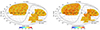 |
Fig. 6. Single Gaussian realization of an LRG map before adding contamination (left panel) and after applying regressis to contaminate the mock (right panel). |
The comparison of angular power spectra is shown in Fig. 7. For CℓκG, we find no significant differences between the contaminated and true power spectra. While the mitigated spectra are systematically lower than the truth, this difference is smaller than the dispersion of the clean mock power spectra (i.e., the  uncertainty). In relative terms, at the lowest multipoles where the fNL signal arises, we find differences between the mitigated and true spectra of up to ∼15%, ∼25%, and ∼30–35% for the fNL = −50, 0, and 50 mocks, respectively. Nonetheless, constraining fNL from CℓκG using uncorrected maps would lead to a much larger
  covariance from the large amount of extra power in CℓGG, significantly increasing the fNL uncertainty. For this reason, we used the mitigated maps as the baseline in our cross-correlation pipeline.
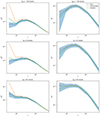 |
Fig. 7. Mean angular power spectra of the full sample LRG autocorrelation (left panels) and LRG-CMB lensing cross-correlation (right panels), computed from the 100 mock realizations used to test our pipeline for various values of fNL (−50 top panels, 0 middle panels, and 50 bottom panels). The blue lines show the true angular power spectra before adding contamination, the shaded blue area corresponds to the dispersion on the true spectra, the orange lines correspond to the angular power spectra of the contaminated mocks, and the green lines to the contaminated mocks after imaging systematics mitigation. |
For CℓGG, the systematics mitigation presents a more complicated picture: we find that for the fNL = 50 mocks the mitigated spectra are compatible with the dispersion of the true spectra, but the performance of the mitigation pipeline depends on fNL: for fNL = −50 and fNL = 0, the first multipole bin of the mitigated spectra is clearly still too high, lying outside the 1σ range of the clean mocks. Thus, for CℓGG we imposed a scale cut of the first five multipoles contained in this bin and adopted ℓmin = 7 for the parameter inference with the mocks and real data. Having a larger ℓmin for CℓGG than for CℓκG also allowed us to put a joint constraint on fNL, while having better control of the systematics.
We then applied the MCMC parameter inference pipeline on the mean of the clean and mitigated angular power spectra of the 100 mock realizations for each value of fNL. We analyzed CℓκG and CℓGG separately and jointly in order to understand the impact of each observable on the constraints, as well as the effects of possible remaining systematics. We list the median likelihood values with 68% confidence intervals in Table 1 for the mocks without systematics (clean) and in Table 2 for the mocks with systematics (mitigated). For the clean mocks, we find almost no intrinsic bias on the recovered fNL values, always having a ≲0.3σ agreement with the input. For the constraints from CℓκG on mocks after contamination and systematics mitigation, the input fNL is always within the 1σ error bars of the measurements on mocks, and the bias on the measured fNL is also lower than 0.5σ for the fNL = 0 and fNL = −50 mocks. The larger disagreement between the measured and true values for the fNL = 50 mocks can be interpreted as a consequence of an overfitted power spectrum after applying the systematics mitigation pipeline (with the bottom right panel of Fig. 7 showing the largest offset between mitigated and clean in the lowest ℓ bin, in units of the standard deviation). For CℓGG, we also find a level of agreement between the measured and true fNL values within 1σ; however, in this case, the highest bias on the measurement happens for the fNL = −50 mocks. For the joint CℓκG + CℓGG tests, using ℓmin = 7 for CℓGG, we find a good agreement for the zero and positive fNL cases, and a ≲1σ bias on the fNL = −50 mocks. Additionally, due to the systematics uncertainties on CℓGG, we measured the constraints from mocks using a joint approach in which we kept the CℓGG information for ℓ > 32 only, in such a way that it constrained the galaxy bias but did not affect the scales where the fNL signal arose.
Median likelihood fNL values with 68% confidence intervals obtained from the application of our analysis pipeline to clean Gaussian mocks with fNL = −50, 0, and 50.
Median likelihood fNL values with 68% confidence intervals obtained from the application of our analysis pipeline to contaminated and mitigated Gaussian mocks with fNL = −50, 0, and 50.
The results of the tests on mocks with systematics reported in Table 2 are driven by the impact of the systematics mitigation on the angular power spectra shown in Fig. 7: for the negative fNL mocks, there is a quite limited (∼15%) overfit on CℓκG and some remaining power for CℓGG, while for positive fNL mocks there is a stronger overfit (≳30%) on CℓκG and the true power spectrum is almost perfectly recovered for CℓGG. In consequence, for the negative fNL mocks, the constraints from CℓκG present almost no bias with respect to the true fNL, while the constraints from CℓGG are biased by ≲1σ toward higher fNL values, likely due to remaining systematics. The opposite behavior is found for the positive fNL mocks: the constraints from CℓκG are biased by ≲1σ, while the constraints from CℓGG present a better accuracy. For the fNL = 0 mocks, we find almost no bias for CℓGG and a 0.5σ bias for CℓκG, also driven by the overfit of systematics mitigation. In the case of the joint constraints, when adopting the baseline ℓmin = 7 for CℓGG, the constraints behave in a similar way to those from the autocorrelation, performing accurately for zero and positive fNL. Our results show that, even if there could be possible biases on fNL due to remaining or overcorrected systematics, the input fNL is within the 1σ uncertainties of the measurement for every single case.
6. Results
We list in Table 3 the median likelihood values with 68% confidence intervals for fNL and b0, obtained from the MCMC analysis applied to CℓκG and CℓGG separately and jointly. We obtain an uncertainty σ(fNL)≲ 40 when using the CℓκG cross-correlation only. Using a scale cut at ℓmin = 7, this uncertainty is reduced to σ(fNL)∼ 25 from CℓGG only and to σ(fNL)∼ 20 from the combination of both observables. The median likelihood values of fNL suggest a preference of this LRG sample for positive values of fNL, which could be interpreted as a consequence of remaining systematics. However, taking into account the error bars, our results are consistent with a ΛCDM universe with Gaussian initial conditions at a ∼1σ level for CℓκG and ≳1σ when combining this information with the LRG autospectra, CℓGG. For the galaxy bias parameter, b0, we obtain a compatible result with previous measurements using this LRG sample: for example, Zhou et al. (2021) measured b0 ∼ 1.5 assuming a redshift evolution proportional to D(z)−1. Fig. 8 shows the 68% and 95% confidence ellipses for the fNL – b0 plane obtained from the two observables and their combination.
Median likelihood fNL and b0 values with 68% confidence intervals obtained from the application of our analysis pipeline to the LRG data and their cross-correlation with the Planck CMB lensing.
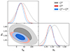 |
Fig. 8. 1σ and 2σ confidence ellipses for the joint posterior distribution of the fNL and b0 parameters obtained from the CℓκG cross-correlation (grey contours), the CℓGG autocorrelation (red contours), and both observables jointly (blue contours). |
We assumed as a baseline fiducial cosmology the σ8 ∼ 0.77 measurement from the cross-correlation between ACT lensing and this LRG sample (Sailer et al. 2024; Kim et al. 2024). As a robustness test, we recomputed the constraints assuming other σ8 values in the literature: the Planck 2018 best-fit value for this parameter, σ8 = 0.811 (Planck Collaboration VI 2020), as well as the DESI full-shape analysis determination, σ8 = 0.842 (DESI Collaboration 2024d) and the measurement from BOSS × Planck CMB lensing, σ8 = 0.688 (Chen et al. 2024). We show in Fig. 9 the comparison between the CℓκG constraints on the fNL – b0 plane assuming the baseline and the alternative values from the literature for σ8. Assuming the Planck 2018, DESI 2024, and BOSS × LRG σ8 best-fit values, we find  ,
,  , and fNL = 40 ± 32, respectively. The median likelihood fNL value is unaffected in every case with respect to the σ8 = 0.77 case listed in Table 3, while the 68% confidence interval is ∼10% larger for the Planck 2018 case (σ8 ∼ 0.81), ∼20% larger for the DESI 2024 case (σ8 ∼ 0.84), and ∼20% smaller for the BOSS × LRG case (σ8 ∼ 0.69). The trend shows larger uncertainties on fNL as a consequence of assuming larger σ8 values. This is essentially due to the degeneracy between the galaxy bias and σ8: higher σ8 values result in lower b0 measurements, and this affects the amplitude of the (b − p) term that enhances the fNL signal (see Eq. (2)).
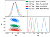 |
Fig. 9. 1σ and 2σ confidence ellipses for the joint posterior distribution of the fNL and b0 parameters obtained from the CℓκG cross-correlation. The green contours assume the baseline σ8 value preferred by the LRG sample used in this paper, while the grey, red, and blue contours assume other σ8 determinations in the literature using Planck 2018, DESI 2024, and BOSS × Planck data, respectively. |
We also tested the robustness of our results to the choice of the fiducial galaxy bias redshift evolution assumed in Eq. (21). For this, we assumed a model in which the galaxy bias evolution was given by bg = b0 × [D(z)]a, and we left the a parameter free, together with fNL, fixing b0 = 1.51 to the best fit in Table 3. We find  and a = −1.01 ± 0.09, obtaining full consistency with the baseline results and the fiducial galaxy bias evolution.
Our baseline analysis assumed the universality relation for the scale-dependent galaxy bias induced by fNL, with a value p = 1 in Eq. (2). However, works on simulations, such as Barreira (2020), suggest a more realistic value for this parameter could be p = 0.55. We recomputed the constraints on fNL from CℓκG, assuming p = 0.55, and compared them to the baseline p = 1 case in Fig. 10. When assuming p = 0.55, we find  . The median likelihood value of fNL is shifted as predicted by Barreira (2020), but the compatibility with ΛCDM remains at the ∼1σ level. Further, we also computed the constraints for a model-independent case in which, instead of assuming the universality relation where bϕ = 2δc(bg − p), no specific form for bϕ is assumed and we constrained the product bϕfNL instead of fNL. In this case, we find
  , a measurement that is still compatible with ΛCDM at the ∼1σ level.
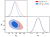 |
Fig. 10. 1σ and 2σ confidence ellipses for the joint posterior distribution of the fNL and b0 parameters obtained from the CℓκG cross-correlation. The red contours correspond to the baseline constraints assuming p = 1, while the blue contours assume p = 0.55, as suggested in Barreira (2020). |
In order to understand the stability of our fNL measurement from CℓκG in terms of systematics, we compare in Fig. 11 the constraints from the Planck lensing – DESI LRG cross-correlation with the case in which no systematics mitigation was performed. In the latter case, we find  . The result is compatible with the baseline case using systematics weights, but the uncertainties are larger due to the impact of the extra CℓGG power spectrum in the covariance matrix. This also emphasizes the importance of performing an accurate systematics mitigation, even for cross-correlation analysis.
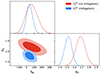 |
Fig. 11. 1σ and 2σ confidence ellipses for the joint posterior distribution of the fNL and b0 parameters obtained from the CℓκG cross-correlation. The blue contours correspond to the baseline constraints after applying the SYSnet mitigation weights to the data and the red contours to the case in which no systematics mitigation was performed. |
We also tested the robustness of our results to the systematics looking at the stability of the results as a function of the minimum multipole, ℓmin. In Fig. 12 we represent the constraints on fNL from CℓκG and CℓGG for ℓmin = 2, 7, and 12. For CℓκG, the constraints are compatible at a ≲1σ level with fNL = 0 for the three ℓmin values. Instead, for CℓGG, we find a ∼1σ deviation for ℓmin = 7, while this deviation rises to ∼2σ for ℓmin = 2 and ℓmin = 12. This indicates that the lower multipoles on  might be dominated by observational systematics, as suggested by the test on mocks, while for CℓκG it is safer to include all the scales in the analysis.
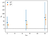 |
Fig. 12. Constraints on fNL from CℓκG (orange dots) and CℓGG (blue dots) with 68% confidence interval as a function of the minimum multipole ℓmin included in the analysis. |
In addition, we tested the compatibility of our results among different regions of the sky. We computed our constraints on fNL by applying masks of the NGC and SGC and list the results in Table 4. We find compatible results between the two galactic caps, and even if the best-fit fNL values we obtain from CℓκG are consistently higher than those measured from the full footprint, the measurements are compatible with zero PNG, considering the larger error bars.
Consistency check for the median likelihood fNL values with 68% confidence intervals obtained from the application of our analysis pipeline to the different sky regions (NGC and SGC) of the LRG data and their cross-correlation with the Planck CMB lensing.
Our constraint on fNL from the DESI LRG – Planck lensing cross-correlation is also compatible with the main result from Rezaie et al. (2024) using the LRG autocorrelation only. Rezaie et al. (2024) discuss in detail the impact of the mitigation recipe on the fNL error bars and best-fit values. They highlight  when applying a more aggressive nonlinear regression for systematics mitigation using nine features maps, while we selected a more conservative treatment in order to avoid a strong overfit in the cross-correlation,
  . When applying the same nonlinear treatment with three maps that we chose for this study, they find
  (before calibration) and fNL = 47 ± 14 (after calibration). We note that, in Rezaie et al. (2024), a calibration of the constraints is proposed, based on the results of the tests on mocks, and that all multipoles were included in the baseline analysis, while we did not apply any calibration and we set ℓmin = 7 for
  . Another important difference in our analysis is the contamination model on the mocks: we used nonlinear weights to implement the contamination on the mocks, while in Rezaie et al. (2024), linear weights were applied to generate this contamination. A calibration of the fNL constraints based on the mocks would be model dependent in any case, and our aim is instead to show the capabilities of
  to produce more stable measurements of fNL, either alone or in combination with
  .
.
7. Conclusions
In this work, we used an LRG catalog from the DESI Legacy imaging surveys, calibrated with the spectroscopic redshifts that have been observed for the DESI Survey Validation, in combination with the Planck PR4 CMB lensing map, to put a constraint on the primordial local non-Gaussianity parameter, fNL. We measured fNL through the scale-dependent bias effect using as observables the cross-correlation between the LRG and CMB lensing maps in the angular domain, CℓκG, and the autocorrelation of the LRG field, CℓGG.
In order to limit the impact of imaging systematics on large scales where the fNL signal is present, we used a neural network code for imaging systematics mitigation. Our measurement was performed without blinding, but the full analysis methodology was tested on mock fields including imaging systematics for different fNL values. Our end-to-end pipeline works at a reasonable level of agreement with the input fNL values, being especially robust when combining both CℓκG and CℓGG for the positive and zero fNL mocks. From the systematics tests on mocks, we find residual contamination in the behavior of the five first multipoles (ℓ = 2 − 6) of CℓGG; hence, we imposed a cut at ℓmin = 7 for the autocorrelation power spectrum.
From the CMB – LRG cross-correlation, CℓκG, alone we find  at the 68% confidence level. We performed some robustness tests on this result, such as changing the fiducial σ8 to other values in the literature, different from the DESI LRG best fit, changing the value of the p parameter, modifying the fiducial bias evolution, or varying the minimum multipole, ℓmin, to evaluate the possible impact of systematics, and we find consistent results for every test. If we combine our result with the information from the angular LRG autocorrelation, CℓGG, adopting the ℓmin = 7 cut, we find
  , although CℓGG presents a larger statistical fluctuation as a function of ℓmin, suggesting that CℓκG is more stable and less sensitive to the effect of imaging systematics. Our results are consistent with the fNL measurements from the DESI LRG by Rezaie et al. (2024) and motivate the future use of CMB cross-correlations, together with the tracers’ autocorrelations and an appropriate systematics mitigation technique, in order to perform accurate fNL measurements.
Data availability
All data points, maps, covariances, and MCMC chains shown in the figures of this paper are publicly available in https://doi.org/10.5281/zenodo.14401463
Acknowledgments
J. R. Bermejo-Climent and R. Demina acknowledge support from the U.S. Department of Energy under the grant DE-SC0008475.0. JRBC acknowledges the support of the Spanish Ministry of Science and Innovation under the grants PID2021-126616NB-I00 and “DarkMaps” PID2022-142142NB-I00, and from the European Union through the grant “UNDARK” of the Widening participation and spreading excellence program (project number 101159929). AK was supported as a CITA National Fellow by the Natural Sciences and Engineering Research Council of Canada (NSERC), funding reference #DIS-2022-568580. MR is supported by the U.S. Department of Energy grants DE-SC0021165 and DE-SC0011840. This material is based upon work supported by the U.S. Department of Energy (DOE), Office of Science, Office of High-Energy Physics, under Contract No. DE-AC02-05CH11231, and by the National Energy Research Scientific Computing Center, a DOE Office of Science User Facility under the same contract. Additional support for DESI was provided by the U.S. National Science Foundation (NSF), Division of Astronomical Sciences under Contract No. AST-0950945 to the NSF’s National Optical-Infrared Astronomy Research Laboratory; the Science and Technology Facilities Council of the United Kingdom; the Gordon and Betty Moore Foundation; the Heising-Simons Foundation; the French Alternative Energies and Atomic Energy Commission (CEA); the National Council of Humanities, Science and Technology of Mexico (CONAHCYT); the Ministry of Science, Innovation and Universities of Spain (MICIU/AEI/10.13039/501100011033), and by the DESI Member Institutions: https://www.desi.lbl.gov/collaborating-institutions. The DESI Legacy Imaging Surveys consist of three individual and complementary projects: the Dark Energy Camera Legacy Survey (DECaLS), the Beijing-Arizona Sky Survey (BASS), and the Mayall z-band Legacy Survey (MzLS). DECaLS, BASS and MzLS together include data obtained, respectively, at the Blanco telescope, Cerro Tololo Inter-American Observatory, NSF’s NOIRLab; the Bok telescope, Steward Observatory, University of Arizona; and the Mayall telescope, Kitt Peak National Observatory, NOIRLab. NOIRLab is operated by the Association of Universities for Research in Astronomy (AURA) under a cooperative agreement with the National Science Foundation. Pipeline processing and analyses of the data were supported by NOIRLab and the Lawrence Berkeley National Laboratory. Legacy Surveys also uses data products from the Near-Earth Object Wide-field Infrared Survey Explorer (NEOWISE), a project of the Jet Propulsion Laboratory/California Institute of Technology, funded by the National Aeronautics and Space Administration. Legacy Surveys was supported by: the Director, Office of Science, Office of High Energy Physics of the U.S. Department of Energy; the National Energy Research Scientific Computing Center, a DOE Office of Science User Facility; the U.S. National Science Foundation, Division of Astronomical Sciences; the National Astronomical Observatories of China, the Chinese Academy of Sciences and the Chinese National Natural Science Foundation. LBNL is managed by the Regents of the University of California under contract to the U.S. Department of Energy. The complete acknowledgments can be found at https://www.legacysurvey.org/. Any opinions, findings, and conclusions or recommendations expressed in this material are those of the author(s) and do not necessarily reflect the views of the U. S. National Science Foundation, the U. S. Department of Energy, or any of the listed funding agencies. The authors are honored to be permitted to conduct scientific research on Iolkam Du’ag (Kitt Peak), a mountain with particular significance to the Tohono O’odham Nation.
References
- Adame, A. G., Avila, S., Gonzalez-Perez, V., et al. 2024, A&A, 689, A69 [NASA ADS] [CrossRef] [EDP Sciences] [Google Scholar]
- Afshordi, N., & Tolley, A. J. 2008, Phys. Rev. D, 78, 123507 [Google Scholar]
- Akrami, Y., Andersen, K. J., Ashdown, M., et al. 2020, A&A, 643, A42 [NASA ADS] [CrossRef] [EDP Sciences] [Google Scholar]
- Alonso, D., Sanchez, J., & Slosar, A. 2019, MNRAS, 484, 4127 [Google Scholar]
- Ballardini, M., Matthewson, W. L., & Maartens, R. 2019, MNRAS, 489, 1950 [NASA ADS] [CrossRef] [Google Scholar]
- Bardeen, J. M., Steinhardt, P. J., & Turner, M. S. 1983, Phys. Rev. D, 28, 679 [Google Scholar]
- Barreira, A. 2020, JCAP, 2020, 031 [CrossRef] [Google Scholar]
- Barreira, A. 2022, JCAP, 2022, 013 [CrossRef] [Google Scholar]
- Bermejo-Climent, J. R., Ballardini, M., Finelli, F., et al. 2021, Phys. Rev. D, 103, 103502 [NASA ADS] [CrossRef] [Google Scholar]
- Cabass, G., Ivanov, M. M., Philcox, O. H. E., Simonović, M., & Zaldarriaga, M. 2022, Phys. Rev. D, 106, 043506 [NASA ADS] [CrossRef] [Google Scholar]
- Cagliari, M. S., Castorina, E., Bonici, M., & Bianchi, D. 2024, JCAP, 2024, 036 [Google Scholar]
- Carbone, C., Verde, L., & Matarrese, S. 2008, ApJ, 684, L1 [Google Scholar]
- Carron, J., Mirmelstein, M., & Lewis, A. 2022, JCAP, 2022, 039 [CrossRef] [Google Scholar]
- Castorina, E., Hand, N., Seljak, U., et al. 2019, JCAP, 2019, 010 [Google Scholar]
- Challinor, A., & Lewis, A. 2011, Phys. Rev. D, 84, 043516 [NASA ADS] [CrossRef] [Google Scholar]
- Chaussidon, E., Yèche, C., Palanque-Delabrouille, N., et al. 2021, MNRAS, 509, 3904 [Google Scholar]
- Chaussidon, E., Yèche, C., de Mattia, A., et al. 2024, ArXiv e-prints [arXiv:2411.17623] [Google Scholar]
- Chen, X. 2010, Adv. Astron., 2010, 638979 [NASA ADS] [CrossRef] [Google Scholar]
- Chen, S.-F., Ivanov, M. M., Philcox, O. H. E., & Wenzl, L. 2024, Phys. Rev. Lett., 133, 231001 [Google Scholar]
- Dalal, N., Doré, O., Huterer, D., & Shirokov, A. 2008, Phys. Rev. D, 77, 123514 [CrossRef] [Google Scholar]
- D’Amico, G., Lewandowski, M., Senatore, L., & Zhang, P. 2025, Phys. Rev. D, 111, 063514 [Google Scholar]
- DESI Collaboration (Aghamousa, A., et al.) 2016a, ArXiv e-prints [arXiv:1611.00037] [Google Scholar]
- DESI Collaboration (Aghamousa, A., et al.) 2016b, ArXiv e-prints [arXiv:1611.00036] [Google Scholar]
- DESI Collaboration (Abareshi, B., et al.) 2022, AJ, 164, 207 [NASA ADS] [CrossRef] [Google Scholar]
- DESI Collaboration (Adame, A. G., et al.) 2024a, AJ, 168, 58 [NASA ADS] [CrossRef] [Google Scholar]
- DESI Collaboration (Adame, A. G., et al.) 2024b, AJ, 167, 62 [NASA ADS] [CrossRef] [Google Scholar]
- DESI Collaboration (Adame, A. G., et al.) 2024c, ArXiv e-prints [arXiv:2411.12021] [Google Scholar]
- DESI Collaboration (Adame, A. G., et al.) 2024d, ArXiv e-prints [arXiv:2411.12022] [Google Scholar]
- DESI Collaboration (Adame, A., et al.) 2025a, JCAP, 2025, 012 [Google Scholar]
- DESI Collaboration (Adame, A., et al.) 2025b, JCAP, 2025, 124 [CrossRef] [Google Scholar]
- DESI Collaboration (Adame, A., et al.) 2025c, JCAP, 2025, 021 [Google Scholar]
- Dey, A., Schlegel, D. J., Lang, D., et al. 2019, AJ, 157, 168 [Google Scholar]
- Flaugher, B., Diehl, H. T., Honscheid, K., et al. 2015, AJ, 150, 150 [Google Scholar]
- Foreman-Mackey, D., Hogg, D. W., Lang, D., & Goodman, J. 2013, PASP, 125, 306 [Google Scholar]
- García-García, C., Alonso, D., & Bellini, E. 2019, JCAP, 2019, 043 [Google Scholar]
- Giannantonio, T., Scranton, R., Crittenden, R. G., et al. 2008, Phys. Rev. D, 77, 123520 [Google Scholar]
- Giusarma, E., Vagnozzi, S., Ho, S., et al. 2018, Phys. Rev. D, 98, 123526 [Google Scholar]
- Gorski, K. M., Hivon, E., Banday, A. J., et al. 2005, ApJ, 622, 759 [Google Scholar]
- Grossi, M., Verde, L., Carbone, C., et al. 2009, MNRAS, 398, 321 [CrossRef] [Google Scholar]
- Guth, A. H. 1981, Phys. Rev. D, 23, 347 [Google Scholar]
- Guth, A. H., & Pi, S.-Y. 1985, Phys. Rev. D, 32, 1899 [Google Scholar]
- Guy, J., Bailey, S., Kremin, A., et al. 2023, AJ, 165, 144 [NASA ADS] [CrossRef] [Google Scholar]
- Hivon, E., Gorski, K. M., Netterfield, C. B., et al. 2002, ApJ, 567, 2 [NASA ADS] [CrossRef] [Google Scholar]
- Hu, W., & Okamoto, T. 2002, ApJ, 574, 566 [CrossRef] [Google Scholar]
- Jeong, D., Komatsu, E., & Jain, B. 2009, Phys. Rev. D, 80, 123527 [Google Scholar]
- Kim, J., Sailer, N., Madhavacheril, M. S., et al. 2024, JCAP, 2024, 022 [CrossRef] [Google Scholar]
- Kitanidis, E., & White, M. 2021, MNRAS, 501, 6181 [NASA ADS] [CrossRef] [Google Scholar]
- Komatsu, E., & Spergel, D. N. 2001, Phys. Rev. D, 63, 063002 [NASA ADS] [CrossRef] [Google Scholar]
- Krolewski, A., Percival, W. J., Ferraro, S., et al. 2024, JCAP, 2024, 021 [Google Scholar]
- Langlois, D. 2010, Inflation and Cosmological Perturbations (Berlin Heidelberg: Springer), 1 [Google Scholar]
- Levi, M., Bebek, C., Beers, T., et al. 2013, ArXiv e-prints [arXiv:1308.0847] [Google Scholar]
- Lewis, A., & Challinor, A. 2011, Astrophysics Source Code Library [record ascl:1102.026] [Google Scholar]
- Limber, D. N. 1953, ApJ, 117, 134 [NASA ADS] [CrossRef] [Google Scholar]
- Miller, T. N., Doel, P., Gutierrez, G., et al. 2024, AJ, 168, 95 [NASA ADS] [CrossRef] [Google Scholar]
- Mueller, E.-M., Rezaie, M., Percival, W. J., et al. 2022, MNRAS, 514, 3396 [NASA ADS] [CrossRef] [Google Scholar]
- Perna, G., Ricciardone, A., Bertacca, D., & Matarrese, S. 2023, JCAP, 10, 014 [Google Scholar]
- Planck Collaboration IX. 2020, A&A, 641, A9 [Google Scholar]
- Planck Collaboration VI. 2020, A&A, 641, A6 [Erratum: A&A 652, C4 (2021)] [NASA ADS] [CrossRef] [EDP Sciences] [Google Scholar]
- Rezaie, M., Seo, H.-J., Ross, A. J., & Bunescu, R. C. 2020, MNRAS, 495, 1613 [Google Scholar]
- Rezaie, M., Ross, A. J., Seo, H.-J., et al. 2024, MNRAS, 532, 1902 [NASA ADS] [CrossRef] [Google Scholar]
- Ross, A. J., Percival, W. J., Carnero, A., et al. 2012, MNRAS, 428, 1116 [Google Scholar]
- Sailer, N., Kim, J., Ferraro, S., et al. 2024, ArXiv e-prints [arXiv:2407.04607] [Google Scholar]
- Schlafly, E. F., Kirkby, D., Schlegel, D. J., et al. 2023, AJ, 166, 259 [NASA ADS] [CrossRef] [Google Scholar]
- Schmittfull, M., & Seljak, U. 2018, Phys. Rev. D, 97, 123540 [NASA ADS] [CrossRef] [Google Scholar]
- Serra, P., Lagache, G., Doré, O., Pullen, A., & White, M. 2014, A&A, 570, A98 [NASA ADS] [CrossRef] [EDP Sciences] [Google Scholar]
- Silber, J. H., Fagrelius, P., Fanning, K., et al. 2023, AJ, 165, 9 [NASA ADS] [CrossRef] [Google Scholar]
- Slosar, A., Hirata, C., Seljak, U., Ho, S., & Padmanabhan, N. 2008, JCAP, 2008, 031 [CrossRef] [Google Scholar]
- Smith, K. M., Zahn, O., & Doré, O. 2007, Phys. Rev. D, 76, 043510 [Google Scholar]
- Starobinsky, A. 1980, Phys. Lett. B, 91, 99 [NASA ADS] [CrossRef] [Google Scholar]
- Starobinsky, A. 1982, Phys. Lett. B, 117, 175 [Google Scholar]
- Takahashi, T. 2014, Prog. Theor. Exp. Phys., 2014, 06B105 [Google Scholar]
- Takahashi, R., Sato, M., Nishimichi, T., Taruya, A., & Oguri, M. 2012, ApJ, 761, 152 [Google Scholar]
- Vazquez Gonzalez, J. A., Padilla, L. E., & Matos, T. 2020, Rev. Mex. Fis. E, 17, 73 [Google Scholar]
- White, M., Zhou, R., DeRose, J., et al. 2022a, JCAP, 2022, 007 [NASA ADS] [CrossRef] [Google Scholar]
- White, M., Zhou, R., DeRose, J., et al. 2022b, JCAP, 02, 007 [Google Scholar]
- Zhou, R., Newman, J. A., Mao, Y.-Y., et al. 2021, MNRAS, 501, 3309 [NASA ADS] [CrossRef] [Google Scholar]
- Zhou, R., Ferraro, S., White, M., et al. 2023a, JCAP, 2023, 097 [CrossRef] [Google Scholar]
- Zhou, R., Dey, B., Newman, J. A., et al. 2023b, AJ, 165, 58 [NASA ADS] [CrossRef] [Google Scholar]
- Zou, H., Zhou, X., Fan, X., et al. 2017, PASP, 129, 064101 [CrossRef] [Google Scholar]
All Tables
Median likelihood fNL values with 68% confidence intervals obtained from the application of our analysis pipeline to clean Gaussian mocks with fNL = −50, 0, and 50.
Median likelihood fNL values with 68% confidence intervals obtained from the application of our analysis pipeline to contaminated and mitigated Gaussian mocks with fNL = −50, 0, and 50.
Median likelihood fNL and b0 values with 68% confidence intervals obtained from the application of our analysis pipeline to the LRG data and their cross-correlation with the Planck CMB lensing.
Consistency check for the median likelihood fNL values with 68% confidence intervals obtained from the application of our analysis pipeline to the different sky regions (NGC and SGC) of the LRG data and their cross-correlation with the Planck CMB lensing.
All Figures
|
Fig. 1. Normalized redshift distribution of the LRG sample, directly measured using the spectroscopic redshifts from DESI Y1 data. |
| In the text | |
|
Fig. 2. Left panel: LRG overdensity field in galactic coordinates, after applying the δ < −30° cut. Right panel: CMB lensing field in galactic coordinates, obtained from the Planck PR4 maps. |
| In the text | |
|
Fig. 3. Angular power spectra of the LRG autocorrelation, CℓGG, and CMB lensing – LRG cross-correlation, CℓκG, obtained from the raw (uncorrected) data and after applying the systematics mitigation pipeline to the LRG maps. |
| In the text | |
|
Fig. 4. Relative impact of the lensing magnification contributions for the CℓGG (blue line) and CℓκG (red line) theoretical angular power spectra obtained with CAMB. |
| In the text | |
|
Fig. 5. Correlation matrix as obtained from the joint covariance matrix for CℓGG and CℓκG computed with the NaMaster code. |
| In the text | |
|
Fig. 6. Single Gaussian realization of an LRG map before adding contamination (left panel) and after applying regressis to contaminate the mock (right panel). |
| In the text | |
|
Fig. 7. Mean angular power spectra of the full sample LRG autocorrelation (left panels) and LRG-CMB lensing cross-correlation (right panels), computed from the 100 mock realizations used to test our pipeline for various values of fNL (−50 top panels, 0 middle panels, and 50 bottom panels). The blue lines show the true angular power spectra before adding contamination, the shaded blue area corresponds to the dispersion on the true spectra, the orange lines correspond to the angular power spectra of the contaminated mocks, and the green lines to the contaminated mocks after imaging systematics mitigation. |
| In the text | |
|
Fig. 8. 1σ and 2σ confidence ellipses for the joint posterior distribution of the fNL and b0 parameters obtained from the CℓκG cross-correlation (grey contours), the CℓGG autocorrelation (red contours), and both observables jointly (blue contours). |
| In the text | |
|
Fig. 9. 1σ and 2σ confidence ellipses for the joint posterior distribution of the fNL and b0 parameters obtained from the CℓκG cross-correlation. The green contours assume the baseline σ8 value preferred by the LRG sample used in this paper, while the grey, red, and blue contours assume other σ8 determinations in the literature using Planck 2018, DESI 2024, and BOSS × Planck data, respectively. |
| In the text | |
|
Fig. 10. 1σ and 2σ confidence ellipses for the joint posterior distribution of the fNL and b0 parameters obtained from the CℓκG cross-correlation. The red contours correspond to the baseline constraints assuming p = 1, while the blue contours assume p = 0.55, as suggested in Barreira (2020). |
| In the text | |
|
Fig. 11. 1σ and 2σ confidence ellipses for the joint posterior distribution of the fNL and b0 parameters obtained from the CℓκG cross-correlation. The blue contours correspond to the baseline constraints after applying the SYSnet mitigation weights to the data and the red contours to the case in which no systematics mitigation was performed. |
| In the text | |
|
Fig. 12. Constraints on fNL from CℓκG (orange dots) and CℓGG (blue dots) with 68% confidence interval as a function of the minimum multipole ℓmin included in the analysis. |
| In the text | |
Current usage metrics show cumulative count of Article Views (full-text article views including HTML views, PDF and ePub downloads, according to the available data) and Abstracts Views on Vision4Press platform.
Data correspond to usage on the plateform after 2015. The current usage metrics is available 48-96 hours after online publication and is updated daily on week days.
Initial download of the metrics may take a while.