| Issue |
A&A
Volume 698, June 2025
|
|
|---|---|---|
| Article Number | A306 | |
| Number of page(s) | 14 | |
| Section | Catalogs and data | |
| DOI | https://doi.org/10.1051/0004-6361/202452685 | |
| Published online | 26 June 2025 | |
Supernovae at distances <40 Mpc
II. Supernova rate in the local Universe
1
Department of Physics, Tsinghua University,
Haidian District,
Beijing
100084,
China
2
Purple Mountain Observatory, Chinese Academy of Sciences,
Nanjing
210023,
China
3
Las Cumbres Observatory,
6740 Cortona Drive Suite 102,
Goleta,
CA
93117-5575,
USA
4
Department of Physics, University of California,
Santa Barbara,
CA
93106-9530,
USA
5
Yunnan Observatories, Chinese Academy of Sciences,
Kunming
650216,
China
6
International Centre of Supernovae, Yunnan Key Laboratory,
Kunming
650216,
PR China
7
School of Physics and Astronomy, Tel Aviv University,
Tel Aviv
69978,
Israel
8
Center for Astrophysics | Harvard & Smithsonian,
60 Garden Street,
Cambridge,
MA
02138-1516,
USA
9
The NSF AI Institute for Artificial Intelligence and Fundamental Interactions,
USA
10
School of Physics and Information Engineering, Jiangsu Second Normal University,
Nanjing
211200,
China
11
Beijing Planetarium, Beijing Academy of Sciences and Technology,
Beijing,
100044,
China
★ Corresponding author: This email address is being protected from spambots. You need JavaScript enabled to view it.
Received:
21
October
2024
Accepted:
2
April
2025
Abstract
Context. This is the second paper of a series aiming to determine the birth rates of supernovae (SNe) in the local Universe.
Aims. We aimed to estimate the SN rates in the local Universe and fit the delay-time distribution of type Ia SNe (SNe Ia) to put constraints on their progenitor scenarios.
Methods. We performed a Monte Carlo simulation to estimate volumetric rates using the nearby SN sample introduced in Paper I. The rate evolution of core-collapse (CC) SNe closely follows the evolution of the cosmic star formation history, while the rate evolution of SNe Ia involves the convolution of the cosmic star formation history and a two-component delay-time distribution including a power law and a Gaussian component.
Results. The volumetric rates of type Ia, Ibc, and II SNe are derived as 0.325 ± 0.040−0.010+0.016, 0.160 ± 0.028−0.014+0.044, and 0.528 ± 0.051−0.013+0.162 (in units of 10−4yr−1 Mpc−3 h703), respectively. The rate of CCSNe (0.688 ± 0.078−0.027+0.0206) is consistent with previous estimates, which trace the star formation history. Conversely, the newly derived local SN Ia rate is larger than existing results given at redshifts 0.01 < z < 0.1, favoring an increased rate from the Universe at z ∼ 0.1 to the local Universe at z < 0.01. A two-component model effectively reproduces the rate variation, with the power law component accounting for the rate evolution at larger redshifts and the Gaussian component with a delay time of 12.63 ± 0.38 Gyr accounting for the local rate evolution. This delayed component, with its exceptionally long delay time, suggests that the progenitors of these SNe Ia were formed around 1 Gyr after the birth of the Universe, which could only be explained by a double-degenerate progenitor scenario. Comparison with the Palomar Transient Factory (PTF) sample of SNe Ia at z = 0.073 and the morphology of their host galaxies, reveals that the increased SN Ia rate at z < 0.01 is primarily due to the SNe Ia of massive E and S0 galaxies with old stellar populations. Based on the above results, we estimate the Galactic SN rate as 3.08 ± 1.29 per century.
Key words: methods: data analysis / surveys / supernovae: general
© The Authors 2025
 Open Access article, published by EDP Sciences, under the terms of the Creative Commons Attribution License (https://creativecommons.org/licenses/by/4.0), which permits unrestricted use, distribution, and reproduction in any medium, provided the original work is properly cited.
This article is published in open access under the Subscribe to Open model. This email address is being protected from spambots. You need JavaScript enabled to view it. to support open access publication.
1 Introduction
The birth rates of different types of supernovae (SNe) and their redshift evolution provide important constraints on SN progenitors and advance our understanding of cosmic chemical evolution. During the 20th century and the first decade of the 21st century, numerous studies have attempted to measure SN rates in local and distant Universe based primarily on targeted surveys of preselected galaxies or sky fields. The conventional procedure is the control-time method (Zwicky 1942; van den Bergh & Tammann 1991; Leaman et al. 2011), which involves the construction of light curve functions for different types of SNe. For each type, the sum of time when the SNe would be brighter than the limiting magnitude of the survey is defined as the control time of the search. The SN rate is then calculated using the total number of discovered samples divided by the control time. It is usually expressed in units of SNu, for instance  , where
  represents the B-band solar luminosity. Using the galaxy luminosity distribution, SN rates expressed in units of SNu can be converted to volumetric rates. However, the sample from target surveys may introduce an observational bias, as they preferentially monitor brighter galaxies.
Before the 1990s, studies of SN rates relied on samples from the Palomar SN search (Zwicky 1942), the Asiago SN search (Cappellaro & Turatto 1988), and Robert Evans’ visual searches (van den Bergh et al. 1987; van den Bergh & McClure 1990). Subsequent work by Cappellaro et al. (1999) compiled an important sample of 137 SNe from historical SN surveys, which became the most valuable for studies of SN rates, host galaxy environments, SN progenitor systems, and cosmic star formation history (Mannucci 2005; Mannucci et al. 2005; Mannucci 2008). Li et al. (2011a) later established a complete sample of 175 SNe and a “full-optimal” SN sample with a total of 726 SNe from the 10-year Lick Observatory Supernova Search (LOSS) program. With this homogeneous set of nearby SNe from a single survey, they derived the most accurate estimates of the fractions of different types of SNe and their corresponding rates in the local Universe at that time. Using data from the Palomar Transient Facility (PTF; Rau et al. 2009; Law et al. 2009), Frohmaier et al. (2019, 2021) provide one of the most updated rate measurements for type Ia and core-collapse supernovae (CCSNe) at z < 0.1.
SN rates at moderate to higher redshifts have been derived using samples from untargeted rolling searches (Dahlen et al. 2004; Dilday et al. 2010; Perrett et al. 2012; Rodney et al. 2014; Cappellaro et al. 2015; Frohmaier et al. 2019, 2021), improving constraints on rate evolution and progenitor systems of different types of SNe. Notably, the evolution of CCSN rates with redshifts is found to align well with the cosmic star formation history (SFH; Hopkins & Beacom 2006; Rujopakarn et al. 2010; Cucciati et al. 2012; Frohmaier et al. 2021), as CCSNe usually originate from massive stars with short lifetimes.
In comparison, the evolution of the type Ia SN (SN Ia) rate does not track the SFH but can be regarded as the convolution of delay-time distribution (DTD) and SFH. The delay time is defined as the duration between the instantaneous burst of star formation and the resulting SN Ia explosions. Among the parameterization models of DTD, a simple power-law model, ∝ t−β with  , is empirically valid (Maoz et al. 2012; Graur & Maoz 2013; Graur et al. 2014). Other models include the functional form of e-folding, Gaussian (Dahlen et al. 2012; Palicio et al. 2024), and the two-component model. A popular form of the two-component model combines a prompt component that tracks the instantaneous star formation rate (SFR) and a delayed component that is proportional to stellar mass (Mannucci 2005). The prompt component represents very young SNe Ia that explode soon after the formation of their progenitors, while the delayed component has longer delay times and corresponds to older stellar population. With reliable measurements of the SN Ia rate with redshift and cosmic SFH, the DTD can be determined by inverting the convolution (Horiuchi & Beacom 2010; Dahlen et al. 2012; Perrett et al. 2012; Graur et al. 2014; Rodney et al. 2014; Frohmaier et al. 2019). Different DTDs can provide insight into the progenitor systems of SNe Ia (Maoz & Mannucci 2012). For example, the double-degenerate (DD) channel with two carbonoxygen white dwarfs (CO WDs) can provide a DTD for normal SNe Ia with an initial peak at around 1 Gyr and a tail up to about 10 Gyr (Pakmor et al. 2013), while most single-degenerate (SD) models predict shorter delay times with few or no SNe Ia produced beyond 2-3 Gyr (Childress et al. 2014; Maoz et al. 2014).
Paper I of this series discusses the construction of the nearby SN and galaxy samples. A total of 211 SNe discovered between 2016 and 2023 are selected within 40 Mpc, comprising 69 SNe Ia, 34 SNe Ibc, and 109 SNe II. In this paper, two galaxy samples are used: the host galaxy sample with 191 galaxies and the Galaxy List for the Advanced Detector Era+ (GLADE+) sample with 8790 galaxies. The Hubble-type distributions of the two galaxy samples show noticeable differences. The most abundant types in the local Universe are the elliptical (E), lenticular (S0), late-type spiral (Scd), and irregular (Irr) galaxies, whereas Sc type spiral galaxies host most SNe. The average stellar mass distribution suggests that galaxies hosting SNe are generally more massive. For all of our SN sample, we obtained their classifications and gave detailed subtype fractions. Then, combined with host galaxy information, we studied the radial and stellar mass distributions of different subtypes and their correlations. The number distribution of SNe in galaxies of different Hubble types was compared to that of the SN sample from Li et al. (2011b). We found clear evidence of a double-peak structure in E-S0 and late-type Sc galaxies for the SN Ia sample. This could suggest a two-component model for SN Ia DTD, with a prompt and a delayed component corresponding to the young and old stellar population in late-type spirals and E-S0 galaxies, respectively.
This is paper II of the series and is organized as follows. In Sect. 2, we present the methodology for estimating local volumetric rates and the final results. In Sect. 3 we calculate the SN rate in galaxies of different Hubble types. We then derive the Milky Way SN rate and, in Sect. 4, we compare our rate measurements with the literature values and derive the DTDs for SNe Ia. The CCSNe rate evolution is fitted with the cosmic star formation history. Conclusions are summarized in Sect. 5.
2 The volumetric supernova rate
In this section, we describe our approach for estimating the volumetric SN rates using the SN sample established in Paper I and discuss their uncertainties.
2.1 Supernova rate estimation
Following the approach proposed by Rodney et al. (2014), we define the observed count Nobs as the observed number of SNe and the control count Nctrl as the expected number of SNe that should be detected if the local SN rates were constant at  . The local volumetric SN rate in units of
  is then given by
 (1)
(1)
The value of Nobs corresponds to SNe detected within 40 Mpc between 2016 and 2023. Monte Carlo simulations were used to calculate Nctrl, where 100 000 SNe were generated for each type (Ia, Ibc and II). For each individual SN, we randomly generated the following set of properties: distance, absolute peak magnitude, host extinction, Galactic extinction, right ascension, declination, and date of peak brightness.
We divided each sample into different subtypes by random sampling using the fractions of Paper I. All SNe were uniformly distributed in a sphere with a radius of 40 Mpc. For each subtype, we generated absolute peak magnitudes based on the bias-corrected Gaussian distributions of B-band peak absolute magnitudes of different subtypes given by Richardson et al. (2014, see our Table B.1 and their Table 1 for detailed parameters for the Gaussian distributions). Based on the subtype fractions estimated in Paper I, we adopted the brightest 5.9% of the generated Ia sample as the 91T sample and the dimmest 17.6% as the 91bg sample, the remainder classified as the normal Ia sample. Since Richardson et al. (2014) did not give the absolute peak magnitude distribution for 02cx-like events, we adopted a uniform distribution between −14.0 and −18.0 mag for this subtype according to the peak magnitude range given by Jha et al. (2017). The host extinction information was generated following Holwerda et al. (2015), for which the distribution of AV is taken as N = N0exp(-AV/0.4). For Galactic extinctions, we used values at randomly generated SN coordinates (i.e., uniformly distributed throughout the sky) according to Schlafly & Finkbeiner (2011). The date of the peak was drawn from a uniform distribution within the range 2016-2023. From the generated properties (i.e., the peak absolute magnitude, distance, host and Galactic extinction values), we calculated the observed peak apparent magnitude for each SN under extinction effect and assessed its detectability.
In Paper I we identified the All-Sky Automated Survey for Supernovae (ASAS-SN; Shappee et al. 2014; Kochanek et al. 2017), the Asteroid Terrestrial-impact Last Alert System (ATLAS; Tonry et al. 2018; Smith et al. 2020), and the Zwicky Transient Facility (ZTF; Masci et al. 2019; Bellm et al. 2019) as the primary discoverers of our SN sample. In the current study, we evaluated whether the generated SNe were detectable by these three surveys, combining the generated peak apparent magnitudes with the light-curve functions given by Li et al. (2011b, see their Table 2 and Figs. 1–3 for detailed light curve templates). Li et al. (2011b) provided 22 templates for SNe Ia, including one each for the 91bg, 91T, and 02cx-like subtypes and 19 for normal Ia, along with three templates for the fast-, slow-, and averageevolving SNe Ibc and one for peculiar SNe Ibc. A single light curve template was constructed for the SNe subtypes IIP, IIL, and IIb, while three templates (fast-, average-, and slow-evolving), were adopted for SNe IIn. We simulated the light-curve evolution for the generated SNe and assessed detectability according to their survey strategies1. For each SN, the light-curve function is randomly chosen from the light curve families of Li et al. (2011b) of the given subtype.
Because the photometric bands of the generated peak absolute magnitudes (B-band), light curve templates (R-band), and surveys (see Appendix B) are all different, we first standardized the peak absolute magnitudes to the R-band to simulate light-curve evolution. We then transformed these R-band magnitudes to each survey’s specific photometric band to determine the detection probability. To achieve this, we needed statistical patterns of the differences in magnitudes between these photometric bands. For SNe Ia, we followed the approach of Nugent et al. (2002)2 who presented the UBVRI magnitude differences from the peak B-band value for different subtypes of SNe Ia from 20 days before to 70 days after the B-band maximum. By stretching the templates (between 0.8 < s < 1.1), we estimated the systematic uncertainties arising from template adoption. For CCSNe, we utilized Pessi et al. (2023)’s B-, V-, and R-band photometric data, which includes detailed subtype classifications, including Ib, Ic, Ic-BL, IIP, IIL, IIb, and IIn (see Appendix G of their paper). The corresponding uncertainties were estimated from peak magnitude errors and post-peak decline rates. Thus, our procedure involved three steps. First, we randomly generated the B-band peak absolute magnitude for an SN. Next, we converted the generated B-band peak magnitudes into the R-band values to fit the light curve templates of Li et al. (2011b). Finally, the generated B-band magnitudes were converted to the values of the corresponding photometric band of the survey to compare with the limiting magnitudes. For the transformation between the R- and o-band magnitudes, we adopted the same method as described in Xiang et al. (2019, see Sect. 3.2 and Fig. 7 for details of the evolution of c - V and o - R colors with respect to evolution phases).
We divided the sky into three regions: Region I represents the observation field of ZTF. Region II covers the observation field of ATLAS excluding the ZTF field. The remainder of the sky is denoted as Region III, which is monitored exclusively by ASAS-SN. If the randomly generated SN was located in Region I, we first determined whether it could be detected by ZTF. If ZTF did not detect the SN, we then evaluated the detection by ATLAS, followed by ASAS-SN. The SN was counted as a nondetection if it was undetectable by the three surveys. Similarly, if the SN was located in region II, we evaluated whether it could be detected by ALTAS and then by ASAS-SN. For SNe in region III, ASAS-SN was the only survey that we considered. The detection efficiencies of the three surveys are provided in Appendix B. For SNe with varying apparent peak magnitudes and light duration, the surveys would detect them at different probabilities. Within the observation window, when an SN was covered by one of the surveys and its brightness exceeded the detection limit, we estimated the possibility of this SN being detected by that survey according to the apparent SN magnitude during observation and the detection efficiency given in Appendix B. For multiple observations in the considered time window, we combined the possibilities of each single observation to give an overall detection probability for the SN (that is, 1-P, where P represents the nondetection probability for all observations). By adding all the possibilities, we calculated a control count according to this fraction. The process was repeated 1000 times to give the mean value and standard deviation.
The values for Nobs and Nctrl are given in Table 1, together with the volumetric rates and the estimated statistical and systematic uncertainties.
Observed counts, control counts and volumetric rates.
2.2 Uncertainties
Uncertainties in the observed count include the statistical error, which is the Poisson noise for the sample, and the systematic error, which mainly arises from three sources: “edge-on” SNe with a distance around 40 Mpc, SNe with uncertain redshifts, and missing SNe in galaxy cores. We determined the contribution of the first two sources using the methodology outlined in Paper I. For bright SNe in bright galaxy cores, the presence of the galaxy core will affect the quality of the observed SNe spectra. However, Desai et al. (2024) argued that for surveys such as ASAS-SN, the signal-to-noise ratio of observation of the SNe in the local Universe is so high that neglecting the host does not affect the detection probability. For faint SNe, the noise is dominated by the sky rather than the host, so the presence of a bright host core has little effect on the detection probability. Furthermore, Holoien et al. (2019) report that multiple SNe have been discovered in central regions of galaxies by ASAS-SN, at distances <0.02 kpc from the galactic nuclei (see their Fig. 2). ZTF and ATLAS can also detect nuclear SNe, with comparable or superior detection capabilities because of their deeper detection limits and finer pixel resolutions compared to ASAS-SN. In our sample, a large number of SNe located within 1 kpc of the center of their hosts (26 out of a total of 211 SNe) were detected by ZTF, ATLAS, and ASAS-SN. As the majority of our SN sample was discovered by ASAS-SN, ATLAS and ZTF (including some amateur surveys), missed detection of SNe near galactic cores should be less significant for our sample. All nearby SNe initially reported by amateur surveys were subsequently confirmed by the above professional surveys within days of their discovery.
For the control count, we considered four sources of systematic error: the Monte Carlo simulation-derived standard deviation of the control count; the assumed distribution of hostgalaxy dust extinctions; dust extinction or obscuration causing a non-negligible fraction of CCSNe to be missed by optical surveys; and uncertainties in the assumed models and distributions, including the subtype fractions, peak absolute magnitude distributions, light-curve templates, photometric band magnitude differences, and survey cadence and limiting magnitudes. The host-galaxy extinction values generated in our simulation may underestimate cases where SNe suffer from severe extinction, leading to overestimated apparent magnitudes, and therefore an overestimation of Nctrl. We revised the Monte Carlo simulations by adjusting the host-galaxy extinction distributions according to the extinction data set of Holwerda et al. (2015, i.e., increasing high extinction values in Fig. 8 of Holwerda et al. 2015 that the exponential formula we adopted failed to fit). The resultant differences in the derived control count were then set as the uncertainty. Similarly, we quantified the uncertainties associated with the fourth source according to the uncertainties of the assumed models and distributions. The impact of the third source was discussed in paper I. We adopted the reported value of 57.16 missed CCSNe and assigned these to SNe Ibc and II based on their relative proportions to estimate the uncertainty caused by this effect.
The final local volumetric rates were calculated as


for SNe Ia, Ibc, and II respectively. And we combine the last two rates to obtain the local volumetric rate for CCSNe:

3 Supernova rate as a function of galaxy Hubble type
3.1 Method
The study of Li et al. (2011a) defines multiple SN subsamples with different associated galaxy samples, including the “full” sample (N = 929), the “full-optimal” sample (N = 726), the “season” sample (N = 656), and the “season-optimal” sample (N = 499), respectively. Li et al. (2011a) used these samples to calculate the supernova rates per unit mass (SNuM) for SNe Ia, Ibc, and II in a fiducial galaxy of different Hubble types. The results of different SN subsamples are consistent with each other within 1σ. Their final rates were calculated using the 726 SNe in the “full-optimal” sample, which provides a good balance between improving small-number statistics and avoiding systematic biases.
Due to our smaller sample size compared to Li et al. (2011a), we were unable to employ their control-time method. In Paper I, we used the SNuM and the rate-size relation given by Li et al. (2011a) to calculate the expected number of SN explosions in all galaxies of the GLADE+ sample. The rate-size relation is given by
 (2)
(2)
where M0 = 4 × 10¹⁰ M⊙ is the stellar mass of the fiducial galaxy and the values of SNuM(M0)3 and RSSM (the rate-size slope, which is the power-law index between the rate and the mass) are provided in Table 4 of Li et al. (2011a). Using Eq. (2), we calculated the SNuM for each galaxy based on its stellar mass of any galaxy, enabling estimation of the expected number of SNe to explode in the galaxy within a given duration of time. Having constructed a complete galaxy sample in the local Universe (i.e., the GLADE+ sample), we reversed the approach to estimate the SNuM for galaxies of each Hubble type.
For a given Hubble type, the SN rate for a fiducial galaxy of that type is given by
 (3)
(3)
where N is the number of SNe in galaxies of the specified Hubble type, RSSM is provided in Table 4 of Li et al. (2011a), T = 8 yr is the survey duration, and  is the sum of stellar mass to the power of (RSSM + 1) over every galaxy of the given Hubble type in our GLADE+ sample.
3.2 Uncertainties
We account for three sources of uncertainties in our analysis. The first is the uncertainty in the number of SNe, previously estimated in Sect. 2. This was accounted for by splitting the total value into the corresponding host galaxy Hubble types. The second arises from errors in the RSS, as detailed in Table 4 of Li et al. (2011a). The third stems from uncertainties in the galaxy stellar mass provided by the GLADE+ sample. These statistical (first) and systematic (second, third) uncertainties were combined to compute the total uncertainties presented in Table 2.
SN rates in fiducial galaxies of different Hubble types.
3.3 Results
Table 2 reports the rates for fiducial-sized galaxies across different Hubble types. In our sample, no CCSNe were found in elliptical galaxies, and no SNe Ibc were found in Irr galaxies. We therefore provide upper limits for these cases. To calculate the rate for a specific galaxy, the stellar mass of the galaxy is applied to Eq. (2).
In Fig. 1, all SNuM rates are plotted as solid circles, and the upper limits are plotted as solid squares. For comparison, we also present the rates estimated by Li et al. (2011a).
The SNuM rates of SNe Ia are consistent with those reported by Li et al. (2011a), being constant across different Hubble-type bins except for Sc galaxies, where the rate appears noticeably high. We examined the properties of the Sc galaxies hosting SNe Ia in our sample and found that the uncertainties of their morphological type codes are small (i.e., <1.0), indicating that their classifications are relatively accurate. Thus, the high SNuM rate of SNe Ia in Sc galaxies could be intrinsic.
The SNuM rates of CCSNe are generally consistent with those reported by Li et al. (2011a). The CCSNe rates are close to 0 in the E, S0, and Sa galaxies. However, SN Ibc rates increase to peak in Sb galaxies and gradually decrease to near-zero levels in Scd and Irr galaxies. This contrasts with the findings of Li et al. (2011a), where SN Ibc rates peak in Sc galaxies and then drop to a non-zero value in Irr galaxies. SN II rates in galaxies of different Hubble types agree well with Li et al. (2011a), except for the significantly higher rate in Sb galaxies and the lower rate in Scd galaxies. In Paper I, we examined the potential causes for the small number of CCSNe in Scd and Irr galaxies in our sample. It is likely that Li et al. (2011a) overestimated the CCSNe rates in Irr and Scd galaxies due to the preference of massive Scd and Irr galaxies in their observation, and plenty of low-mass Scd and Irr galaxies could be missed in their “full” galaxy sample. Our smaller SN Ibc sample might also contribute to the discrepancy. Figs. 8 and 9 in Paper I show that the average stellar mass of Sb galaxies in the SN-host galaxy sample is smaller than that in the GLADE+ sample. Furthermore, the number of CCSNe discovered in Sb galaxies is also larger compared to Li et al. (2011a). This suggests that more CCSNe tend to explode in less massive galaxies, which naturally results in a higher CCSN rate in Sb galaxies. We note that for the SNuM calculation via the control-time method, a large sample size is needed.
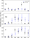 |
Fig. 1 Supernova (SN) rates (for a galaxy of the fiducial size) for galaxies of different Hubble types (solid circles). Upper limits for SNe that are not found in galaxies of the corresponding Hubble type are shown as solid squares. The blue circles indicate the SN rates given by Li et al. (2011a). |
3.4 The Galactic SN rate
We estimated the expected SN rate in the Milky Way (hereafter, the Galactic SN rate) from the SN rates we derived from the 40-Mpc sample. We assumed that the Hubble type of the Milky Way is Sbc (van den Bergh & McClure 1994). For the stellar mass, we adopted the value of 4.81 ± 0.13 × 10¹⁰ M⊙ (Lian et al. 2024). In comparison, according to Li et al. (2011a), we can assume that the size of the Milky Way is similar to that of the Andromeda galaxy (M31) or the average size of the Sbc galaxies in the “optimal” LOSS galaxy sample of Leaman et al. (2011). Using the rate-size relation of Eq. (2), we calculated the Galactic SN rate in units of SNe per century, with the relevant results presented in Table 3.
The Galactic SN rate derived from the stellar mass of the Milky Way, given by Lian et al. (2024), is 3.08 ± 1.29 SNe per century. This is intermediate between the estimates based on the stellar masses suggested by Li et al. (2011b), and consistent with the value of 2.84 ± 0.60 SNe per century obtained by Li et al. (2011a). Our result is also in good agreement with the published range of 1.4-5.8 SNe per century derived through different methods (van den Bergh & Tammann 1991; van den Bergh & McClure 1994).
Galactic SN rate.
4 Analysis
4.1 Comparison with historical results
We compared our SN Ia and CCSN rates with historical results, primarily derived from targeted surveys, such as Li et al. (2011a). These surveys tend to monitor brighter, more massive galaxies, and thus introduce bias in the observed SN population due to correlations between the light curves of SNe and their host galaxy properties (Sullivan et al. 2010). The final volumetric rates would also be affected by such a bias. For comparison, we also include recent results of untargeted rolling searches, such as PTF (Frohmaier et al. 2019) and ASAS-SN (Desai et al. 2024). These results, unlike those of targeted surveys, are less susceptible to observational bias and achieve greater precision.
4.1.1 Type Ia supernovae
Fig. 2 compares our SN Ia rate with published rates from Cappellaro et al. (1999), Hardin et al. (2000), Madgwick et al. (2003), Blanc et al. (2004), Dahlen et al. (2004), Barris & Tonry (2006), Botticella et al. (2008), Dilday et al. (2008), Horesh et al. (2008), Dilday et al. (2010), Li et al. (2011a), Perrett et al. (2012), Rodney et al. (2014), Cappellaro et al. (2015), Frohmaier et al. (2019), Perley et al. (2020), Sharon & Kushnir (2022), and Desai et al. (2024), adjusted to the assumed cosmological model. The local SN Ia rate measurements are summarized in Table 4, and all rate measurements used in this work are provided in Table C.2.
Our rate is plotted as a red star with a value slightly larger than the results given by Li et al. (2011a) at a confidence level of approximately 1σ. However, we achieve better precision (smaller uncertainty) compared to most local rate estimations, similar to the recent values of Frohmaier et al. (2019). The SN Ia rate experiences a rapid decline from redshift z = 0 to z ∼ 0.1, followed by a gradual increase to z ∼ 1, before again decreasing. The unusual rate decrease from z = 0 to z ∼ 0.1 is discussed and possible explanations are described in Sects. 4.2 and 4.4.
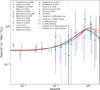 |
Fig. 2 Volumetric SN Ia rates compared to historical measurements at different redshifts. Red and black lines denote the SN Ia rates derived from power-law and e-folding forms of the DTD, respectively. The dashed, solid, and dotted lines illustrates the SN Ia rates derived from SFH given by Yüksel et al. (2008), Li (2008), and Harikane et al. (2022), respectively. |
4.1.2 Core-collapse supernovae
Our CCSN rate is compared to the historical results of Dahlen et al. (2004), Cappellaro et al. (2005), Botticella et al. (2008), Bazin et al. (2009), Li et al. (2011a), Botticella et al. (2012), Dahlen et al. (2012), Melinder et al. (2012), Taylor et al. (2014), Cappellaro et al. (2015), Graur et al. (2015), Strolger et al. (2015), and Frohmaier et al. (2021). The published values, scaled to the adopted Hubble constant, are shown in Fig. 3. Local CCSN rate measurements are summarized in Table 4, and all rate measurements used in this work are provided in Table C.1. Our rate is well consistent with that given by Li et al. (2011a) but with slightly higher precision.
4.2 The delay-time distribution
In this section, we introduce the application of our improved nearby SN Ia rate measurement. The evolution of SN Ia rate should follow the SFH, but because of the long evolution timescale of their progenitor system, the SN Ia DTD should be taken into account. The SN Ia rate can be modeled as the convolution of the DTD and the SFH:
 (4)
(4)
where t′ - t is the delay time, t is the look-back time corresponding to the redshift at which we evaluate the SN Ia rate, tF is the look-back time corresponding to the redshift zF, where the first stars formed. We set zF = 10, μ is the scale factor, and Ψ(t) is the DTD.
First, we used a power-law DTD, Ψ(t) = t−β, and an efolding DTD, Ψ(t) = exp(-t/τ), to fit our data, where τ is the characteristic delay time for the e-folding DTD. For the SFH, we adopted the functional forms of Yüksel et al. (2008) and Harikane et al. (2022), and the piecewise form of Li (2008) given in Eqs. (5)–(7), respectively:
![Mathematical equation: \mathrm{SFH}(z) = \mathrm{SFH}_0 \left[(1 + z)^{a\eta} + \left(\frac{1 + z}{\mathrm{B}}\right)^{b\eta} + \left(\frac{1 + z}{\mathrm{C}}\right)^{c\eta}\right]^{\frac{1}{\eta}}, \label{SFH1}](/articles/aa/full_html/2025/06/aa52685-24/aa52685-24-eq65.png) (5)
(5)
with a = 3.4, b = −0.3, c = −3.5, SFH0 = 0.02 M⊙yr−1Mpc−3, B ≃ 5000, C ≃ 9, and η ≃ −10.
 (6)
(6)
 (7)
(7)
The resulting best-fit parameters are listed in Table 5 and the SNRs derived from Eq. (4) for each SFH model are shown in Fig. 2.
All models presented in Fig. 2 fit well with the overall rate measurements. All power-law models yield β ∼ 1, consistent with historical fittings (i.e., β = 1.13 ± 0.05 from Wiseman et al. 2021). This power-law DTD is consistent with a progenitor scenario of DD (Maoz & Mannucci 2012; Graur & Maoz 2013). All e-folding models favor a characteristic delay timescale of around 2 Gyr. Strolger et al. (2020) also derived a family of delay-time distribution solutions from the volumetric SN Ia rate evolution and suggested an exponential distribution similar to the β ∼ 1 power-law distribution, consistent with our results. However, none of these models reproduce the rapid decline in SN Ia rate observed from the Universe between z = 0 and z ≃ 0.1. Recent high-precision measurements from the ASAS-SN and PTF projects at < z > = 0.024 and 0.073 suggest that this short decline could be an intrinsic trend. Inspired by the double-peak structure identified in Paper I, we examined another DTD model, the two-component model.
The most popular two-component model is the “A+B” model which consists of a prompt component that tracks instantaneous star formation and a delayed component that is proportional to Mstellar (Mannucci 2005):
 (8)
(8)
The A and B coefficients scale the delayed and prompt components, respectively. However, the delayed component of this A+B model needs to be converted to a DTD using the relation between Mstellar and time. The star formation component consists of SNe Ia that explode immediately after the formation of their progenitor systems, with no delay time, since it is proportional to the SFH. However, this zero-delay time is unrealistic for SNe Ia. Given that the DTD of the power-law function adequately reproduces the evolution of the SN la rate from z ∼ 0.1 to larger redshifts, we introduced another functional form of DTD combining a power-law component plus a Gaussian component. The power-law component contributes to the SN Ia rate at large redshifts, while the Gaussian component is the correction for the decline in the SN Ia rate in the local Universe:
 (9)
(9)
where τ is the mean delay time of the Gaussian component, and a and b represent the normalization parameters. The corresponding best fit parameters are listed in Table 6 and the SNRs derived from Eq. (4) using different SFH models are shown in Fig. 4.
All three models successfully reproduce the SN Ia rate evolution at z > 0.1, as well as the rate decline in the local Universe, whereas a single-component DTD model (i.e., the power-law and Gaussian DTD model) failed to provide adequate fits. The powerlaw components all give β ∼ 1, consistent with the historical results of the single power-law DTD model, and correspond to the prompt part of the two-component model with delay times close to 0. The delayed component of all three models exhibits delay times of ∼12.5 Gyr. We adopt the best fit value from the Yüksel et al. (2008) model, yielding β = 1.18 ± 0.04 and τ = 12.63 ± 0.38 (corresponding to a redshift of z ∼ 6 for the assumed cosmological parameters). This result suggests a large number of star-forming galaxies at z ∼ 6. We present details of the two-component model of Yüksel et al. (2008) SFH in Fig. 5. The unusual rate increase from z ∼ 0.1 to the local Universe can be attributed to the Gaussian component with a long delay time.
Recent observations of JWST have revealed an increasing number of galaxies at z > 6 (Jaskot et al. 2024), with some having redshifts beyond 12 and out to 14 (Chakraborty et al. 2024; Lu et al. 2025). The JWST Advanced Deep Extragalactic Survey (JADES) discovered a sample of 79 SNe in the JADES Deep Field, which contains many high-redshift SNe, with seven at z ≥ 4,15 at z ≥ 3 and 38 at z ≥ 2 (DeCoursey et al. 2025). The sample includes a spectroscopically-confirmed SN Ia at z = 2.90 (Pierel et al. 2024), and a SN IIP at z = 3.61, representing the highest-redshift SNe Ia and SN IIP ever discovered. The presence of SNe at high redshifts suggests star-formation activities in evolved galaxies at even higher redshifts. Furthermore, historical studies on the host galaxies of SNe Ia have shown that their metallicity is systematically higher than that of CCSNe (Shao et al. 2014; Galbany et al. 2016). The relatively high metallicity environment suggests that the birth of zero-metallicity first-generation stars could be much earlier, considering the non-negligible delay time of SNe Ia. Thus, a delay time of 12.63 Gyr is plausible. In summary, JWST observations favor the presence of long delay times in the formation of SNe Ia, consistent with our analysis. We explore the origin of the local Universe’s rate decline in Sect. 4.4.
The DTD-fitting results provide insight into SNe Ia progenitor systems. The DTD of the SD channel exhibits a sharp cutoff at 2-3 Gyr (Han & Podsiadlowski 2004). According to Wang & Han (2010b), SD models produce SNe Ia across a wide delaytime distribution, where the WD + He star channel contributes to the SNe Ia with delay times shorter than 100 Myr, while the WD + MS and WD + RG channels contribute to those with age longer than 1 Gyr, but with a very small fraction longer than 3 Gyr. The WD + MS channel also contributes to the SNe Ia with intermediate delay times around 100 Myr-1 Gyr. While the SD channel cannot account for our delayed component, it still has a potential contribution to the prompt component. For the DD channel, the models give a delay time ranging from several Gyr to around 10 Gyr (Pakmor et al. 2013; Crocker et al. 2017; Zenati 2019). The model simulations by Ruiter et al. (2009); Wang & Han (2010a) showed that the SNe Ia from the DD channel has delay times of a few Myr - 15 Gyr. The DTD of the DD channel peaks at several hundred Myr, followed by a power-law decline ∝ t−1, which corresponds to the power-law component of our model. The tail extends to ∼15 Gyr, with an event rate approximately 2 orders of magnitude lower than the peak value. From their model simulations, we can conclude that the DD channel could account for both the prompt and the delayed components of our two-component DTD model. However, these models all predict a power-law decline for the DD channel, with a very small event rate for delay times greater than 10 Gyr. While they allow for the possibility of a 12.63 ± 0.38 Gyr delay time for the DD progenitor systems, none can explain the Gaussian component observed at large delay times in our model. Briel et al. (2022) estimated SN Ia rate using models of Binary Population And Spectral Synthesis (BPASS; Eldridge et al. 2017; Stanway & Eldridge 2018), deriving the DTD of SNe Ia across metallicities (see their Fig. 1). At solar metallicity, the delay time exhibits a distinct second peak at an age greater than 10 Gyr. Joshi et al. (2024) analyzed the DTD of SNe Ia across host galaxy samples, identifying that a significant component exists in the DTD bin around 12 Gyr, for host galaxies with no star formation over the past 10 Gyr (see their Fig. 3). Both studies indicated the existence of a group of SNe Ia with extremely long delay times. However, further investigation of the stellar evolution models for the DD channel is encouraged to explore this problem.
Local volumetric SN rates.
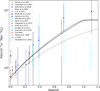 |
Fig. 3 CCSN rates following the methodology of Fig. 2. The dashed, solid, and dotted black lines show the CCSN rates derived from SFH given by Yüksel et al. (2008), Li (2008), and Harikane et al. (2022), respectively. |
Best-fit parameters for the power-law and e-folding DTD convolved with different SFH models.
Best-fit parameters for the two-component models.
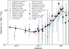 |
Fig. 4 Supernova rates derived using different SFH models and best-fit parameters of the two-component model. The dashed, solid, and dotted lines correspond to the SFH given by Yüksel et al. (2008), Li (2008) and Harikane et al. (2022), respectively. The black dots represent the binned rate measurements used in our DTD fitting procedure. |
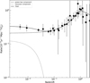 |
Fig. 5 Two-component model of Yüksel et al. (2008) SFH. The solid line represents the best-fit evolution of SN Ia rate while the dashed and dotted lines correspond to the power-law (prompt) and Gaussian (delayed) components, respectively. |
4.3 Star formation rates
For CCSNe, the relationship between their birth rate and SFH is straightforward. Since their progenitors are massive stars with relatively short lifetimes, the SNR of CCSNe should be proportional to the SFH.
Assuming a Salpeter initial mass function (IMF; Salpeter 1955), Ψ(M), over the range 0.1 < M/M⊙ < 125, where all stars with masses in the range 8 < M/M⊙ < 50 explode as SNe, we can calculate the relation between the SFH (in units of M⊙yr−1Mpc−3) and the SNR of CCSNe (in units of yr−1Mpc−3),
 (10)
(10)
where

We normalized the SFH as parameterized by Yüksel et al. (2008), Li (2008) and Harikane et al. (2022) using Eq. (10). Figure 3 shows the resulting SN rate. The CCSN rate follows the same trend as the SFH given by Yüksel et al. (2008) and Li (2008) from z = 0 to around 1 (a look-back time of ∼7.7 Gyr), consistent with the conclusion of Briel et al. (2022). However, the SFH derived by Harikane et al. (2022) significantly underestimates the CC rates. Our local rate measurements match cosmic SFH values from the literature. Better-constrained rate measurements of high-redshift (z > 1) CCSNe will further improve our understanding of SFH.
Both Mannucci et al. (2007) and Mattila et al. (2012) suggested that optical surveys miss a large fraction of CCSNe even in the nearby Universe due to dust obscuration. Mattila et al. (2012) quantified the evolution of the missing CCSNe fraction in the redshift, rising from  at z = 0 to
  at z = 2.0 (see their Table 10 for details). Although surveys such as ZTF, ATLAS, and ASAS-SN have significantly improved systematic SNe detection, the effect of dust obscuration remains non-negligible, even at small distances. Jencson et al. (2018) discovered a type II SN with Spitzer/IRAC during the ongoing SPitzer InfraRed Intensive Transients Survey (SPIRITS). This SN, named SPIRITS 16tn, is located in the nearby galaxy NGC 3556, at 8.8 Mpc, yet it was completely missed by optical searches due to heavy extinction. This implies that CCSNe birth rates may be systematically higher than those estimated from the cosmic star formation history.
4.4 Comparison to the PTF SN Ia sample
To further investigate the anomalous evolution of the SN Ia rate in the local Universe, we compared the host environments of our SN Ia sample and the Frohmaier et al. (2019) sample from the PTF survey (with an average redshift of 0.073). We estimated the host galaxy properties (i.e., host metallicity and stellar mass) of the PTF sample following the same methodology outlined in Sect. 4.2 of Paper I.
The correlation between host metallicity and Hubble type is shown in Fig. 6. Linear fit of the two samples reveal clear differences, with the fraction of E-S0 galaxies in our sample being significantly higher, resulting in higher metallicity at the elliptical end. The slopes of the two lines are ∼0.09 ± 0.02 for our sample and ∼0.06 ± 0.03 for the PTF sample, respectively. Moreover, the PTF SNe Ia sample shows a different Hubble-type distribution with a clear preference for spiral galaxies rather than E-S0 galaxies (upper panel of Fig. 6). A Kolmogorov-Smirnov (K-S) test revealed a p value of 0.04, suggesting that this difference is statistically significant. The lack of SNe Ia in metal-rich E-S0 galaxies with old stellar population in the PTF sample reflects the lower birth rates at redshift ∼0.1 compared to the local Universe. We further investigated the host stellar mass, with the cumulative fractions of host metallicity and the stellar mass distribution of the two samples presented in Figs. 7 and 8.
The PTF SN Ia sample at an average redshift of 0.073 shows an obvious preference for metal-poor and less massive galaxies compared to our local sample of SNe Ia. A K-S test yielded p values of 0.167 and 0.073 for the host metallicity and stellar mass distribution of the two samples, respectively. This further confirms a metal-poor environment for the SN Ia population with a redshift ∼0.1 compared to the local population. As shown in Fig. 1 of Briel et al. (2022), the fraction of SNe Ia with long delay times (>10 Gyr) is significantly higher for metalrich populations. Thus, the group of SNe Ia with long delay times contribute more to the local SN Ia rate, which is consistent with our findings. Furthermore, the host stellar mass of the PTF sample is significantly lower than that of our sample, considering the PTF sample’s lack of E-S0 host galaxies and the fact that E-S0 galaxies are, on average, massive evolved galaxies that typically harbor old stellar populations. We conclude that the higher SN Ia rate at z - 0 originates mainly from massive E-S0 galaxies. Moreover, E-S0 galaxies have older stellar populations than late-type spirals, so the SNe Ia exploding in these galaxies predominantly contribute to the delayed component with long delay times. As shown in Sect. 4.2, the high SN Ia rate in the local Universe is primarily driven by a Gaussian DTD component centered at a delay time of ∼12.5 Gyr. This aligns with the greater prevalence of SNe Ia exploding in metal-rich, massive E-S0 galaxies at z - 0 compared to the PTF sample at z = 0.073.
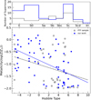 |
Fig. 6 Number of SNe in galaxies of different Hubble types (upper panel) and host metallicity versus Hubble type correlations (lower panel). Blue data represent our sample; black data denote the PTF sample. Linear fits are shown as solid blue (our sample) and dashed black (PTF) lines. |
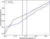 |
Fig. 7 Cumulative fractions for host metallicity distributions of our SN Ia sample (blue) and the sample of Frohmaier et al. (2019). The vertical dashed lines show the average values of the host metallicity for the two SNe Ia samples. |
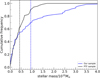 |
Fig. 8 Cumulative fractions for host stellar mass distributions of our SNe Ia sample (blue) and the sample of Frohmaier et al. (2019). The vertical dashed lines show the average values of the host stellar mass for the two SNe Ia samples. |
5 Conclusions
In this paper, we present the local volumetric rates for SN Ia and CCSNe. We used the SN sample from Paper I and performed a Monte Carlo simulation to estimate the local volumetric rate for each SN type. Uncertainties involved with the Monte Carlo simulation were also estimated. We find the SN Ia rate in the local Universe to be
![Mathematical equation: \[\mathrm{SNR_{Ia} = 0.325\pm0.040^{+0.016}_{-0.010} \times 10^{-4} yr^{-1} Mpc^{-3} h^3_{70}},\]](/articles/aa/full_html/2025/06/aa52685-24/aa52685-24-eq76.png)
and the local volumetric rate for CCSNe is
![Mathematical equation: \[ \mathrm{SNR_{CC} = 0.688\pm0.078^{+0.206}_{-0.027} \times 10^{-4} yr^{-1} Mpc^{-3} h^3_{70}}.\]](/articles/aa/full_html/2025/06/aa52685-24/aa52685-24-eq77.png)
The results are consistent with recent rate measurements, although the SN Ia rate is relatively higher. We achieved precision comparable to the PTF and ASAS-SN surveys, representing a significant improvement over most prior studies.
Combined with the GLADE+ sample, we computed supernova rates as a function of galaxy Hubble type. The SNuM rates of SNe Ia, Ibc, and II for galaxies with fiducial size are generally consistent with Li et al. (2011a), except for the noticeable higher SN Ia rate in Sc galaxies. Although this excess is consistent with the number distribution in Paper I, the SNuM rate for SN Ia in E-S0 galaxies does not show the peak structure seen in the number distribution. The significantly lower SN Ibc rate in Scd and Irr galaxies compared to Li et al. (2011a) may reflect either the limited sample size for SNe Ibc or that Li et al. (2011a) overestimated the rate due to their focus on massive Scd and Irr galaxies, and thus the absence of abundant low mass galaxies. Furthermore, we estimated the Galactic SN rate to be 3.08 ± 1.29 SNe per century, which is in good agreement with historical measurements of 1.4-5.8 SNe per century.
Finally, we combined our result with literature SN rates up to higher redshifts. We used the cosmic SN Ia rate evolution to constrain power-law, e-folding and two-component DTD models. The DTD models were convolved with three different SFHs: Yüksel et al. (2008), Li (2008), and Harikane et al. (2022). Although power-law and e-folding DTD models fit the overall rate evolution, they failed to predict the significant decline from z = 0 to ∼0.1 in the local Universe, instead predicting a nearly constant rate. The two-component DTD model provided a suitable fit to the rate evolution with similar values of χ2. Critically, this model reproduced the observed SN la rate decline in the local Universe with two components: a prompt component following the power-law distribution and a delayed Gaussian component centered at a delay time of 12.63 ± 0.38 Gyr, suggesting the existence of star-forming galaxies at z > 6. This two-component model is consistent with the double-peak structure we identified in the Hubble-type distribution of SNe Ia in Paper I. The delayed component’s long delay time favors the DD channel, consistent with previous model simulations. Recent studies further confirm the existence of SNe Ia with extremely long delay times. By comparing the host environment of our SN Ia sample with that of the PTF sample at an average redshift of 0.073, we found that the higher SN Ia rate in the local Universe compared to z ∼ 0.1 originates primarily from SNe Ia exploding in massive E-S0 galaxies with old stellar populations. This further supports the existence of a group of SN Ia with very large delay times (corresponding to the Gaussian component in our two-component model). Our local CCSN rate aligns with theoretical predictions based on cosmic SFHs from the literature.
Our study reveals a severe bias affecting nearby SNe discovered in recent years beyond 40 Mpc. Only the sample within this distance appears to be relatively complete. Future rolling search surveys could better constrain rate measurements beyond z = 0.01 and improve our understanding of DTDs and progenitor systems of SNe Ia.
Data availability
The data underlying this article will be shared on reasonable request with the corresponding author.
Acknowledgements
We acknowledge the support of the staff of Lijiang 2.4m and Xinglong 2.16-m telescopes. This work is supported by the National Science Foundation of China (NSFC grants 12288102, 12033003, and 11633002), the science research grant from the China-Manned Space Project No. CMS-CSST-2021-A12, and the Tencent Xplorer prize. This work makes use of observations from the Las Cumbres Observatory global telescope network. The LCO group is supported by NSF grants AST-1911225 and AST-1911151. D.D.L. is supported by the National Key R&D Program of China (Nos. 2021YFA1600403 and 2021YFA1600400), the National Natural Science Foundation of China (No. 12273105, 12288102), the Youth Innovation Promotion Association CAS (No. 2021058), the Yunnan Revitalization Talent Support Program – Young Talent project, and the Yunnan Fundamental Research Projects (Nos 202401AV070006 and 202201AW070011). We acknowledge the usage of the HyperLeda database (http://leda.univ-lyon1.fr). H.L. is supported by the National Natural Science Foundation of China (NSFC, Grant No. 12403061) and the innovative project of “Caiyun Post-doctoral Project” of Yunnan Province.
Appendix A Detection efficiency of the three surveys
In this section we present the detection efficiencies for the three surveys, (i.e., ZTF, ATLAS, and ASAS-SN), adopted in this work.
In Fig. A.1 we present the histograms of 5σ limiting magnitudes of ZTF, the figure is adopted from Bellm et al. (2019). Median 5σ limiting magnitudes are 20.8 mag in g-band, 20.6 mag in r-band, and 19.9 mag in i-band.
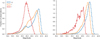 |
Fig. A.1 Left: Histogram of 5σ limiting magnitudes in 30 second exposures for g (blue), r (orange), and i (red) bands over one lunation. Right: Limiting magnitudes for observations obtained within 3 days of new moon. This is Fig.. 6 from Bellm et al. (2019). |
In Fig. A.2 we present the histograms of 5σ limiting magnitudes of ATLAS, the figure is adopted from Smith et al. (2020). Median 5σ limiting magnitudes for each of the systems are 19.0 mag (ATLAS-HKO o band), 19.6 mag (ATLAS-HKO c band), and 19.0 mag (ATLAS MLO o band). With these distributions we compare the apparent magnitude of an SN to calculate the probability of this SN being detected at >5σ above the background noise by these two surveys and hence the probability that the 5a limiting magnitude is dimmer than the SN.
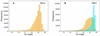 |
Fig. A.2 A: Histogram of 5a limiting magnitudes for MLO in the o band.B:Same as in A,but for HKO with the c and o bands plotted together. This is Fig. 8 from Smith et al. (2020). |
In Fig. A.3 we present the detection completeness as a function of peak apparent magnitude mV,peak for ASAS-SN, the figure is adopted from Desai et al. (2024). The standard choice for the limiting magnitude is mV,lim = 17 mag, where the completeness is ∼ 50%. For SN with peak apparent magnitude outside the values given in Fig. A.3, we did a linear interpolation to determine the completeness curve.
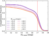 |
Fig. A.3 Completeness as a function of peak apparent magnitude mV,peak with the peak absolute magnitudes MV,peak shown in different colors. The vertical dashed red line marks our standard choice for the limiting magnitude, mV,lim = 17 mag, where the completeness is ∼ 50%. This is Fig. 4 from Desai et al. (2024). |
Appendix B Peak absolute magnitude distributions of different sub-types
Bias-corrected B-band peak absolute magnitude distributions of different sub-types given by Richardson et al. (2014).
Appendix C Summary of SN rate measurements
All CCSN rate measurements used in this work.
All SN Ia rate measurements used in this work.
References
- Barris, B. J., & Tonry, J. L. 2006, ApJ, 637, 427 [CrossRef] [Google Scholar]
- Bazin, G., Palanque-Delabrouille, N., Rich, J., et al. 2009, A&A, 499, 653 [NASA ADS] [CrossRef] [EDP Sciences] [Google Scholar]
- Bellm, E. C., Kulkarni, S. R., Graham, M. J., et al. 2019, PASP, 131, 018002 [Google Scholar]
- Blanc, G., Afonso, C., Alard, C., et al. 2004, A&A, 423, 881 [NASA ADS] [CrossRef] [EDP Sciences] [Google Scholar]
- Botticella, M. T., Riello, M., Cappellaro, E., et al. 2008, A&A, 479, 49 [NASA ADS] [CrossRef] [EDP Sciences] [Google Scholar]
- Botticella, M. T., Smartt, S. J., Kennicutt, R. C., et al. 2012, A&A, 537, A132 [NASA ADS] [CrossRef] [EDP Sciences] [Google Scholar]
- Briel, M. M., Eldridge, J. J., Stanway, E. R., Stevance, H. F., & Chrimes, A. A. 2022, MNRAS, 514, 1315 [NASA ADS] [CrossRef] [Google Scholar]
- Cappellaro, E., & Turatto, M. 1988, IAU Colloq., 101, 489 [Google Scholar]
- Cappellaro, E., Evans, R., & Turatto, M. 1999, A&A, 351, 459 [NASA ADS] [Google Scholar]
- Cappellaro, E., Riello, M., Altavilla, G., et al. 2005, A&A, 430, 83 [NASA ADS] [CrossRef] [EDP Sciences] [Google Scholar]
- Cappellaro, E., Botticella, M. T., Pignata, G., et al. 2015, A&A, 584, A62 [NASA ADS] [CrossRef] [EDP Sciences] [Google Scholar]
- Chakraborty, P., Sarkar, A., Wolk, S., et al. 2024, MNRAS, submitted [arXiv:2406.05306] [Google Scholar]
- Childress, M. J., Wolf, C., & Zahid, H. J. 2014, MNRAS, 445, 1898 [Google Scholar]
- Crocker, R. M., Ruiter, A. J., Seitenzahl, I. R., et al. 2017, Nat. Astron., 1, 0135 [NASA ADS] [CrossRef] [Google Scholar]
- Cucciati, O., Tresse, L., Ilbert, O., et al. 2012, A&A, 539, A31 [NASA ADS] [CrossRef] [EDP Sciences] [Google Scholar]
- Dahlen, T., Strolger, L.-G., Riess, A. G., et al. 2004, ApJ, 613, 189 [NASA ADS] [CrossRef] [Google Scholar]
- Dahlen, T., Strolger, L.-G., Riess, A. G., et al. 2012, ApJ, 757, 70 [NASA ADS] [CrossRef] [Google Scholar]
- DeCoursey, C., Egami, E., Pierel, J. D. R., et al. 2025, ApJ, 979, 250 [Google Scholar]
- Desai, D. D., Kochanek, C. S., Shappee, B. J., et al. 2024, MNRAS, 530, 5016 [NASA ADS] [CrossRef] [Google Scholar]
- Dilday, B., Kessler, R., Frieman, J. A., et al. 2008, ApJ, 682, 262 [Google Scholar]
- Dilday, B., Smith, M., Bassett, B., et al. 2010, ApJ, 713, 1026 [NASA ADS] [CrossRef] [Google Scholar]
- Eldridge, J. J., Stanway, E. R., Xiao, L., et al. 2017, PASA, 34, e058 [Google Scholar]
- Frohmaier, C., Sullivan, M., Nugent, P. E., et al. 2019, MNRAS, 486, 2308 [CrossRef] [Google Scholar]
- Frohmaier, C., Angus, C. R., Vincenzi, M., et al. 2021, MNRAS, 500, 5142 [Google Scholar]
- Galbany, L., Stanishev, V., Mourão, A. M., et al. 2016, A&A, 591, A48 [NASA ADS] [CrossRef] [EDP Sciences] [Google Scholar]
- Graur, O., & Maoz, D. 2013, MNRAS, 430, 1746 [NASA ADS] [CrossRef] [Google Scholar]
- Graur, O., Rodney, S. A., Maoz, D., et al. 2014, ApJ, 783, 28 [NASA ADS] [CrossRef] [Google Scholar]
- Graur, O., Bianco, F. B., & Modjaz, M. 2015, MNRAS, 450, 905 [NASA ADS] [CrossRef] [Google Scholar]
- Han, Z., & Podsiadlowski, P. 2004, MNRAS, 350, 1301 [CrossRef] [Google Scholar]
- Hardin, D., Afonso, C., Alard, C., et al. 2000, A&A, 362, 419 [NASA ADS] [Google Scholar]
- Harikane, Y., Ono, Y., Ouchi, M., et al. 2022, ApJS, 259, 20 [NASA ADS] [CrossRef] [Google Scholar]
- Holoien, T. W. S., Brown, J. S., Vallely, P. J., et al. 2019, MNRAS, 484, 1899 [NASA ADS] [CrossRef] [Google Scholar]
- Holwerda, B. W., Reynolds, A., Smith, M., & Kraan-Korteweg, R. C. 2015, MNRAS, 446, 3768 [NASA ADS] [CrossRef] [Google Scholar]
- Hopkins, A. M., & Beacom, J. F. 2006, ApJ, 651, 142 [NASA ADS] [CrossRef] [Google Scholar]
- Horesh, A., Poznanski, D., Ofek, E. O., & Maoz, D. 2008, MNRAS, 389, 1871 [NASA ADS] [CrossRef] [Google Scholar]
- Horiuchi, S., & Beacom, J. F. 2010, ApJ, 723, 329 [Google Scholar]
- Jaskot, A. E., Silveyra, A. C., Plantinga, A., et al. 2024, ApJ, 973, 111 [NASA ADS] [CrossRef] [Google Scholar]
- Jencson, J. E., Kasliwal, M. M., Adams, S. M., et al. 2018, ApJ, 863, 20 [Google Scholar]
- Jha, S. W., Camacho, Y., McCully, C., & Foley, R. 2017, AAS Meeting Abstracts, 229, 410.01 [Google Scholar]
- Joshi, B. A., Strolger, L.-G., & Zenati, Y. 2024, ApJ, 974, 15 [Google Scholar]
- Kochanek, C. S., Shappee, B. J., Stanek, K. Z., et al. 2017, PASP, 129, 104502 [Google Scholar]
- Law, N. M., Kulkarni, S. R., Dekany, R. G., et al. 2009, PASP, 121, 1395 [NASA ADS] [CrossRef] [Google Scholar]
- Leaman, J., Li, W., Chornock, R., & Filippenko, A. V. 2011, MNRAS, 412, 1419 [NASA ADS] [CrossRef] [Google Scholar]
- Li, L.-X. 2008, MNRAS, 388, 1487 [NASA ADS] [CrossRef] [Google Scholar]
- Li, W., Chornock, R., Leaman, J., et al. 2011a, MNRAS, 412, 1473 [NASA ADS] [CrossRef] [Google Scholar]
- Li, W., Leaman, J., Chornock, R., et al. 2011b, MNRAS, 412, 1441 [NASA ADS] [CrossRef] [Google Scholar]
- Lian, J., Zasowski, G., Chen, B., et al. 2024, Nat. Astron., 8, 1302 [Google Scholar]
- Lu, S., Frenk, C. S., Bose, S., et al. 2025, MNRAS, 536, 1018 [Google Scholar]
- Madgwick, D. S., Hewett, P. C., Mortlock, D. J., & Wang, L. 2003, ApJ, 599, L33 [Google Scholar]
- Mannucci, F. 2005, ASP Conf. Ser., 342, 1604 [Google Scholar]
- Mannucci, F. 2008, Chinese J. Astron. Astrophys. Suppl., 8, 143 [Google Scholar]
- Mannucci, F., Della Valle, M., Panagia, N., et al. 2005, A&A, 433, 807 [NASA ADS] [CrossRef] [EDP Sciences] [Google Scholar]
- Mannucci, F., Della Valle, M., & Panagia, N. 2007, MNRAS, 377, 1229 [NASA ADS] [CrossRef] [Google Scholar]
- Maoz, D., & Mannucci, F. 2012, PASA, 29, 447 [NASA ADS] [CrossRef] [Google Scholar]
- Maoz, D., Mannucci, F., & Brandt, T. D. 2012, MNRAS, 426, 3282 [NASA ADS] [CrossRef] [Google Scholar]
- Maoz, D., Mannucci, F., & Nelemans, G. 2014, ARA&A, 52, 107 [Google Scholar]
- Masci, F. J., Laher, R. R., Rusholme, B., et al. 2019, PASP, 131, 018003 [Google Scholar]
- Mattila, S., Dahlen, T., Efstathiou, A., et al. 2012, ApJ, 756, 111 [Google Scholar]
- Melinder, J., Dahlen, T., Mencía Trinchant, L., et al. 2012, A&A, 545, A96 [NASA ADS] [CrossRef] [EDP Sciences] [Google Scholar]
- Nugent, P., Kim, A., & Perlmutter, S. 2002, PASP, 114, 803 [NASA ADS] [CrossRef] [Google Scholar]
- Pakmor, R., Kromer, M., Taubenberger, S., & Springel, V. 2013, ApJ, 770, L8 [Google Scholar]
- Palicio, P. A., Matteucci, F., Della Valle, M., & Spitoni, E. 2024, A&A, 689, A203 [NASA ADS] [CrossRef] [EDP Sciences] [Google Scholar]
- Perley, D. A., Fremling, C., Sollerman, J., et al. 2020, ApJ, 904, 35 [NASA ADS] [CrossRef] [Google Scholar]
- Perrett, K., Sullivan, M., Conley, A., et al. 2012, AJ, 144, 59 [NASA ADS] [CrossRef] [Google Scholar]
- Pessi, T., Prieto, J. L., Anderson, J. P., et al. 2023, A&A, 677, A28 [NASA ADS] [CrossRef] [EDP Sciences] [Google Scholar]
- Pierel, J. D. R., Engesser, M., Coulter, D. A., et al. 2024, ApJ, 971, L32 [Google Scholar]
- Rau, A., Kulkarni, S. R., Law, N. M., et al. 2009, PASP, 121, 1334 [NASA ADS] [CrossRef] [Google Scholar]
- Richardson, D., Jenkins, Robert L. I., Wright, J., & Maddox, L. 2014, AJ, 147, 118 [NASA ADS] [CrossRef] [Google Scholar]
- Rodney, S. A., Riess, A. G., Strolger, L.-G., et al. 2014, AJ, 148, 13 [Google Scholar]
- Ruiter, A. J., Belczynski, K., & Fryer, C. 2009, ApJ, 699, 2026 [Google Scholar]
- Rujopakarn, W., Eisenstein, D. J., Rieke, G. H., et al. 2010, ApJ, 718, 1171 [NASA ADS] [CrossRef] [Google Scholar]
- Salpeter, E. E. 1955, ApJ, 121, 161 [Google Scholar]
- Schlafly, E. F., & Finkbeiner, D. P. 2011, ApJ, 737, 103 [Google Scholar]
- Shao, X., Liang, Y. C., Dennefeld, M., et al. 2014, ApJ, 791, 57 [Google Scholar]
- Shappee, B., Prieto, J., Stanek, K. Z., et al. 2014, AAS Meeting Abstracts, 223, 236.03 [Google Scholar]
- Sharon, A., & Kushnir, D. 2022, MNRAS, 509, 5275 [Google Scholar]
- Smith, K. W., Smartt, S. J., Young, D. R., et al. 2020, PASP, 132, 085002 [Google Scholar]
- Stanway, E. R., & Eldridge, J. J. 2018, MNRAS, 479, 75 [NASA ADS] [CrossRef] [Google Scholar]
- Strolger, L.-G., Dahlen, T., Rodney, S. A., et al. 2015, ApJ, 813, 93 [NASA ADS] [CrossRef] [Google Scholar]
- Strolger, L.-G., Rodney, S. A., Pacifici, C., Narayan, G., & Graur, O. 2020, ApJ, 890, 140 [NASA ADS] [CrossRef] [Google Scholar]
- Sullivan, M., Conley, A., Howell, D. A., et al. 2010, MNRAS, 406, 782 [NASA ADS] [Google Scholar]
- Taylor, M., Cinabro, D., Dilday, B., et al. 2014, ApJ, 792, 135 [Google Scholar]
- Tonry, J. L., Denneau, L., Flewelling, H., et al. 2018, ApJ, 867, 105 [NASA ADS] [CrossRef] [Google Scholar]
- van den Bergh, S., & McClure, R. D. 1990, ApJ, 359, 277 [Google Scholar]
- van den Bergh, S., & McClure, R. D. 1994, ApJ, 425, 205 [Google Scholar]
- van den Bergh, S., & Tammann, G. A. 1991, ARA&A, 29, 363 [NASA ADS] [CrossRef] [Google Scholar]
- van den Bergh, S., McClure, R. D., & Evans, R. 1987, ApJ, 323, 44 [Google Scholar]
- Wang, B., & Han, Z. 2010a, A&A, 515, A88 [NASA ADS] [CrossRef] [EDP Sciences] [Google Scholar]
- Wang, B., & Han, Z. 2010b, Ap&SS, 329, 293 [Google Scholar]
- Wiseman, P., Sullivan, M., Smith, M., et al. 2021, MNRAS, 506, 3330 [NASA ADS] [Google Scholar]
- Xiang, D., Wang, X., Mo, J., et al. 2019, ApJ, 871, 176 [Google Scholar]
- Yüksel, H., Kistler, M. D., Beacom, J. F., & Hopkins, A. M. 2008, ApJ, 683, L5 [CrossRef] [Google Scholar]
- Zenati, Y. 2019, in Compact White Dwarf Binaries, eds. G. H. Tovmassian, & B. T. Gansicke, 34 [Google Scholar]
- Zwicky, F. 1942, ApJ, 96, 28 [NASA ADS] [CrossRef] [Google Scholar]
ASAS-SN: automatically surveying the entire visible sky every night down to about 18 mag, more details can be seen in Shappee et al. (2014) and Kochanek et al. (2017). ATLAS covers about 24 500 deg2 of the sky in the declination range -45° < δ < +90° with a cadence of 2 days, with four exposures (over a 1-hour interval) reaching ∼19.5 mag in the o band when the sky is dark and seeing is good (see details in Tonry et al. 2018 and Smith et al. 2020). ZTF scans the entire northern visible sky (δ ⩾ -31° and |b| > 7°) every three nights (since the end of 2020, the ZTF public survey has increased its observing cadence to 2 days) at a rate of ∼3760 deg2/hour to median depths of g ∼ 20.8 and r ∼ 20.6 mag, see Masci et al. (2019) and Bellm et al. (2019) for more details. We particularly notice that the ZTF scheduling algorithm is publicly available under an open source license: https://github.com/ZwickyTransientFacility/ztf_sim
Photometric data in UBVRI bands available in https://c3.lbl.gov/nugent/nugent_templates.html
It represents the SN rate in the fiducial galaxy.
All Tables
Best-fit parameters for the power-law and e-folding DTD convolved with different SFH models.
Bias-corrected B-band peak absolute magnitude distributions of different sub-types given by Richardson et al. (2014).
All Figures
|
Fig. 1 Supernova (SN) rates (for a galaxy of the fiducial size) for galaxies of different Hubble types (solid circles). Upper limits for SNe that are not found in galaxies of the corresponding Hubble type are shown as solid squares. The blue circles indicate the SN rates given by Li et al. (2011a). |
| In the text | |
|
Fig. 2 Volumetric SN Ia rates compared to historical measurements at different redshifts. Red and black lines denote the SN Ia rates derived from power-law and e-folding forms of the DTD, respectively. The dashed, solid, and dotted lines illustrates the SN Ia rates derived from SFH given by Yüksel et al. (2008), Li (2008), and Harikane et al. (2022), respectively. |
| In the text | |
|
Fig. 3 CCSN rates following the methodology of Fig. 2. The dashed, solid, and dotted black lines show the CCSN rates derived from SFH given by Yüksel et al. (2008), Li (2008), and Harikane et al. (2022), respectively. |
| In the text | |
|
Fig. 4 Supernova rates derived using different SFH models and best-fit parameters of the two-component model. The dashed, solid, and dotted lines correspond to the SFH given by Yüksel et al. (2008), Li (2008) and Harikane et al. (2022), respectively. The black dots represent the binned rate measurements used in our DTD fitting procedure. |
| In the text | |
|
Fig. 5 Two-component model of Yüksel et al. (2008) SFH. The solid line represents the best-fit evolution of SN Ia rate while the dashed and dotted lines correspond to the power-law (prompt) and Gaussian (delayed) components, respectively. |
| In the text | |
|
Fig. 6 Number of SNe in galaxies of different Hubble types (upper panel) and host metallicity versus Hubble type correlations (lower panel). Blue data represent our sample; black data denote the PTF sample. Linear fits are shown as solid blue (our sample) and dashed black (PTF) lines. |
| In the text | |
|
Fig. 7 Cumulative fractions for host metallicity distributions of our SN Ia sample (blue) and the sample of Frohmaier et al. (2019). The vertical dashed lines show the average values of the host metallicity for the two SNe Ia samples. |
| In the text | |
|
Fig. 8 Cumulative fractions for host stellar mass distributions of our SNe Ia sample (blue) and the sample of Frohmaier et al. (2019). The vertical dashed lines show the average values of the host stellar mass for the two SNe Ia samples. |
| In the text | |
|
Fig. A.1 Left: Histogram of 5σ limiting magnitudes in 30 second exposures for g (blue), r (orange), and i (red) bands over one lunation. Right: Limiting magnitudes for observations obtained within 3 days of new moon. This is Fig.. 6 from Bellm et al. (2019). |
| In the text | |
|
Fig. A.2 A: Histogram of 5a limiting magnitudes for MLO in the o band.B:Same as in A,but for HKO with the c and o bands plotted together. This is Fig. 8 from Smith et al. (2020). |
| In the text | |
|
Fig. A.3 Completeness as a function of peak apparent magnitude mV,peak with the peak absolute magnitudes MV,peak shown in different colors. The vertical dashed red line marks our standard choice for the limiting magnitude, mV,lim = 17 mag, where the completeness is ∼ 50%. This is Fig. 4 from Desai et al. (2024). |
| In the text | |
Current usage metrics show cumulative count of Article Views (full-text article views including HTML views, PDF and ePub downloads, according to the available data) and Abstracts Views on Vision4Press platform.
Data correspond to usage on the plateform after 2015. The current usage metrics is available 48-96 hours after online publication and is updated daily on week days.
Initial download of the metrics may take a while.