| Issue |
A&A
Volume 689, September 2024
|
|
|---|---|---|
| Article Number | A203 | |
| Number of page(s) | 16 | |
| Section | Extragalactic astronomy | |
| DOI | https://doi.org/10.1051/0004-6361/202449740 | |
| Published online | 13 September 2024 | |
Cosmic Type Ia supernova rate and constraints on supernova Ia progenitors
1
Université Côte d’Azur, Observatoire de la Côte d’Azur, CNRS, Laboratoire Lagrange, Bd de l’Observatoire, CS 34229, 06304
Nice cedex 4, France
2
Dipartimento di Fisica, Sezione di Astronomia, Università di Trieste, Via G. B. Tiepolo 11, I-34143
Trieste, Italy
3
I.N.A.F. Osservatorio Astronomico di Trieste, via G.B. Tiepolo 11, 34131
Trieste, Italy
4
I.N.F.N. Sezione di Trieste, via Valerio 2, 34134
Trieste, Italy
5
INAF - Osservatorio Astronomico di Capodimonte, Salita Moiariello 16, I-80131
Napoli, Italy
6
ICRANet, Piazza della Repubblica 10, I-65122
Pescara, Italy
Received:
26
February
2024
Accepted:
19
June
2024
Abstract
Context. Type Ia supernovae play a key role in the evolution of galaxies by polluting the interstellar medium with a fraction of iron peak elements larger than that released in the core-collapse supernova events. Their light curve, moreover, is widely used in cosmological studies as it constitutes a reliable distance indicator on extragalactic scales. Among the mechanisms proposed to explain the Type Ia supernovae (SNe), the single- and double-degenerate channels are thought to be the dominant ones, which implies a different distribution of time delays between the progenitor formation and the explosion.
Aims. In this paper, we aim to determine the dominant mechanism by comparing a compilation of Type Ia SN rates with those computed from various cosmic star-formation histories coupled with different delay-time distribution functions. We also evaluate the relative contributions of both channels.
Methods. By using a least-squares fitting procedure, we modeled the observations of Type Ia SN rates assuming different combinations of three recent cosmic star-formation rates and seven delay-time distributions. The goodness of these fits are statistically quantified by the χ2 test.
Results. For two of the three cosmic star-formation rates, the single degenerate scenario provides the most accurate explanation for the observations, while a combination of 34% single-degenerate- and 66% double-degenerate delay-time distributions is more plausible for the remaining tested cosmic star-formation rates.
Conclusions. Though dependent on the assumed cosmic star-formation rate, we find arguments in favor of the single-degenerate model. From the theoretic point of view, at least ∼34% of the Type Ia SN must have been produced through the single-degenerate channel to account for the observations. The wide, double-degenerate mechanism slightly under-predicts the observations at redshift z ≳ 1, unless the cosmic SFR flattens in that regime. On the contrary, although the purely close double-degenerate scenario can be ruled out, we cannot rule out a mixed scenario with single- and double-degenerate progenitors.
Key words: supernovae: general / galaxies: evolution / galaxies: high-redshift
Corresponding author; This email address is being protected from spambots. You need JavaScript enabled to view it. .
© The Authors 2024
 Open Access article, published by EDP Sciences, under the terms of the Creative Commons Attribution License (https://creativecommons.org/licenses/by/4.0), which permits unrestricted use, distribution, and reproduction in any medium, provided the original work is properly cited.
This article is published in open access under the Subscribe to Open model. This email address is being protected from spambots. You need JavaScript enabled to view it. to support open access publication.
1. Introduction
The study of Type Ia supernovae (SNe) has significant implications for the cosmology and galactic astronomy, allowing us to construct the Hubble diagram at low and high redshifts to constrain some cosmological parameters (e.g., Hamuy et al. 1995; Perlmutter & Aldering 1998; Perlmutter et al. 1999a, 1999b; Riess et al. 1998; Sullivan et al. 2011; Suzuki et al. 2012; Ganeshalingam et al. 2013; Betoule et al. 2014; Rest et al. 2014, and Khetan et al. 2021) and, as major producers of iron (Greggio & Renzini 1983; Matteucci & Greggio 1986), to model the chemical evolution of galaxies among other applications (see review by Ruiz-Lapuente 2014). Given this variety of applications, understanding the nature of their progenitors is crucial. In the past years, many Type Ia SN progenitor models have been proposed both theoretically and empirically, in which the most common scenarios are the double-degenerate (DD) and single-degenerate (SD) channels (see Livio & Mazzali 2018 for a recent review), although other alternatives have emerged to account for some observations (see review of Soker 2024 and references therein). The SD scenario was originally proposed by Whelan & Iben (1973) and consists of a system formed by a C-O white dwarf (WD) plus a normal star that, evolving into a red giant, transfers material over the WD (Wheeler & Hansen 1971; Nomoto 1982a, 1982b). The WD then explodes when its mass reaches the Chandrasekhar mass limit (∼1.44 M⊙). In the DD scenario, originally proposed by Iben & Tutukov (1994 but see also Kato & Hachisu 2012; Kato et al. 2015), two WDs in a binary system merge after emission of gravitational waves and explode when reaching the Chandrasekhar mass (Tutukov & Iungelson 1976; Tutukov & Yungelson 1979; Webbink 1984). The relative contribution of the two main Type Ia SN mechanisms has been controversial historically, with no fully satisfactory scenario (Livio 2000; Greggio et al. 2008; Valiante et al. 2009; Matteucci et al. 2009; Bonaparte et al. 2013; Maoz et al. 2014; Ruiz-Lapuente 2019). Originally, the preferred explosion mechanism was the C-deflagration of the Chandrasekhar WD, but later other possible mechanisms were proposed in order to account for a variety of Type Ia SN types; these required a different exploding mass and also involved He and C detonation besides C deflagration (see Hillebrandt et al. 2013 for a review). The discovered variety of Type Ia SNe required different amounts of 56Ni to power the light curve; for a while, this created uncertainty concerning the possibility of using the Type Ia SNe as standard candles. However, Phillips (1993) discovered a relation between the magnitude at the maximum of Type Ia SNe and that after 15 days, which allows us to still use these SNe as standard candles.
The delay between the progenitor formation and its ultimate explosion is statistically determined by the delay-time distribution (DTD; initially introduced by Madau et al. (1998a, see their Figure 2)) for Type Ia SN. Its first publication in its complete analytical formulation was found through the work of Greggio (2005). Such a DTD can have an analytical form and can describe either the classical SD and DD models or other empirical laws derived from direct observations of Type Ia SNe.
In this work, we treated neither the chemical evolution nor the explosion mechanisms, but the progenitors of these systems. More precisely, we aim to compute the cosmic Type Ia SN rate (Ne yr−1 Mpc−3) by adopting observed cosmic star-formation rates (CSFRs) convolved with a variety of delay-time distribution functions associated with different progenitor models. We tested several suggested CSFRs, such as those of Madau & Dickinson (2014), Harikane et al. (2022), and Kim et al. (2024), and seven different DTD functions: the DTD of Matteucci & Recchi (2001) for the SD model; the wide and close DTDs of Greggio (2005) for the DD model; and the empirically derived ones proposed by Totani et al. (2008), Mannucci et al. (2006), Pritchet et al. (2008), and Strolger et al. (2005). By comparing the predicted cosmic Type Ia rates against the observational data at different redshifts, we put constraints on the best DTD and, therefore, on the best progenitor model for Type Ia SNe. In the previous years, Bonaparte et al. (2013), Graur et al. (2014), Rodney et al. (2014), and Strolger et al. (2020) presented similar works adopting different CSFRs and DTDs, both theoretical and observed (Madau et al. 1998b). Here, we adopt the most recent data on Type Ia SN cosmic rate.
The paper is organized as follows. In Sect. 2, we introduce the notion of the Type Ia SN rate computed by means of various adopted DTDs functions. In Sect. 3, we present the best fits to the observed CSFRs together with the computation of the cosmic Type Ia SN rate. In Sect. 4, we describe the observational data and a comparison between observations and theory. In Sect. 5, we present and discuss the theoretical results compared to the observations at different redshifts. Finally, in Sect. 6 we draw some conclusions.
2. The DTD functions
The DTD function for a Type Ia SN was first proposed by Greggio (2005), and in the following we adopt the same formalism as in that paper. The Type Ia SN rate, RSNIa, can be written as
 (1)
(1)
where kα is the number of stars per unit mass in a stellar generation and is determined by the initial mass function (IMF) as:
 (2)
(2)
The denominator of this expression is the normalization condition of the IMF and is equal to one. Here, we adopted the Salpeter (1955) IMF, which is the same IMF adopted to derive the CSFRs that we use to compute the cosmic Type Ia SN rate. The quantity ϕ(m) is the IMF, and it is chosen to agree with that adopted in deriving the CSFR, as we see in the following Section. The masses in the integration limits are ML = 0.1 M⊙ and MU = 100 M⊙. The quantity ψ(t) is the star formation rate (SFR). The quantity DTD(t) is the assumed DTD function. It is defined in a range of times (τi, τx), which represent the minimum and maximum explosion times for the SNe Ia. The DTD represents an instantaneous burst of star formation and therefore needs to be convolved with the SFR in order to obtain the SN rate. The quantity AIa represents the fraction of systems exploding as Type Ia SNe relative to all the stars defined for the mass range of the IMF. Although AIa might vary with redshift due to a possible dependence on metallicity, we assume it to be constant, as per usual practice (Matteucci 2021), since there is no consensus on a precise metallicity dependence. On one hand, if the metallicity of the accreted gas is ≲ − 1 dex, the wind from the WD is too weak to trigger a Type Ia SN explosion (Kobayashi et al. 1998; Kobayashi & Nomoto 2009). On the other hand, the fraction of close binaries is higher in metal-poor populations (El-Badry & Rix 2018; Moe et al. 2019). Furthermore, the cosmic Type Ia SN rates computed in Kobayashi et al. (1998) for the scenarios with and without such metallicity dependence show small differences at redshift z ≲ 1.2, where the majority of our sample lies (see Tables 1 and B.1). Similarly, we assume that the shape of the DTD does not change with metallicity, although variations are observed in the SD scenario compared to the DD scenario (Meng et al. 2011; Meng & Yang 2012), which is less affected by metallicity. In Fig. 1, we show the different DTD(t) functions adopted in this paper. As one can see in Mannucci et al. (2006, hereafter MVP06), the fraction of prompt Type Ia SNe (those exploding during the first 100 Myr from the beginning of star formation) is as large as 50%, whereas in Strolger et al. (2005, hereafter S05), there are no prompt Type Ia SNe. In all the other DTDs the fraction of prompt Type Ia SNe is below 20%. It is worth noting the power-law trend at late times of Totani et al. (2008, hereafter T08) DTD; the one of Matteucci & Recchi (2001, hereafter MR01); and those of Greggio (2005) for the wide and close DD scenarios (hereafter G05Wide and G05Close, respectively).
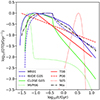 |
Fig. 1. Different DTD functions assumed in this work: Matteucci & Recchi (2001, solid blue curve); Mannucci et al. (2006, dotted green curve); wide and close from Greggio (2005, dashed blue and solid green curves, respectively); Totani et al. (2008, solid red curve); Pritchet et al. (2008, dashed red curve); and Strolger et al. (2005, dotted red curve). The optimal combination of DTDs detailed in Sect. 5.2 is denoted by the dotted-dashed black line. All the distributions are normalized by their maximum. |
Averages of SN rates used in this work.
The T08 DTD has a form of ∼t−1 and was proposed to match the Type Ia SN DTDs inferred from a sample of old, faint, variable objects detected in the Subaru/XMM-Newton Deep Survey (SXDS, Furusawa et al. 2008) at z ∼ 0.4 − 1.2. Similarly, Pritchet et al. (2008) found that a power law with an index of –1/2 accounts for the Type Ia SN rates reported by Sullivan et al. (2006) from the Supernova Legacy Survey (SNLS, Astier et al. 2006). Using a Bayesian maximum likelihood method, Strolger et al. (2004) concluded that a Gaussian DTD better fits the redshift distribution of Type Ia SNe inferred from the Hubble Higher z Supernova Search project (HHZSS, Schmidt et al. 1998) and the Great Observatories Origins Deep Survey (GOODS, Giavalisco et al. 2004). On the contrary, Mannucci et al. (2006) found evidence of a bimodal DTD, where prompt Type Ia SN explosions peak at approximately 50 Myr after progenitor formation, while the remaining events follow a more extended exponential distribution with a timescale of 3 Gyr. The analytic formulations of the DTDs proposed by Matteucci & Recchi (2001) and Greggio (2005) for the SD and DD scenarios, respectively, are characterized by a plateau at early times followed by a power-law decreasing trend (see Fig. 1). Due to their complexity, we refer the reader to their respective papers for detailed explanations.
3. The CSFR and the calculation of the cosmic Type Ia rate
The CSFR is the star formation rate in a unitary volume of the Universe and contains the SFR of a mixture of galaxies. It depends on the distribution of galaxies as a function of redshift. Several attempts to model the CSFR have appeared in the past years, and they take into account precise cosmological scenarios of galaxy formation. For example, in Gioannini et al. (2017), the SFR of galaxies of different morphological types (ellipticals, spirals, and irregulars) were computed by means of detailed chemical-evolution models, then these histories of star formation were convolved with the number density of galaxies as a function of redshift. The galaxy number density was assumed either to be constant in time (pure luminosity evolution) or to vary with redshift following the paradigm of the hierarchical galaxy formation.
Among the prescriptions for a hierarchical formation, the best number density evolution resulted an empirical one, as derived by Pozzi et al. (2015), which provided a theoretical CSFR in excellent agreement with the observationally derived CSFR by Madau & Dickinson (2014). Here we only adopted observationally derived CSFRs (in units of M⊙ yr−1 Mpc−3) and, in particular, the CSFR of Madau & Dickinson (2014), the one of Harikane et al. (2022), and that of Kim et al. (2024). The best fits of these empirically derived CSFRs are shown in Fig. 2. As one can see, the CSFRs are very similar in the z = 3 − 0 redshift range, whereas they differ for z > 3.
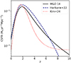 |
Fig. 2. Curves here represent adopted CSFRs derived by the best fit to observations as a function of redshift. The solid black line shows the CSFR of Madau & Dickinson (2014), the dashed blue line corresponds to the CSFR of Harikane et al. (2022), while the dotted red line represents the CSFR of Kim et al. (2024). |
In order to compute the cosmic rate of SNe Ia (RIaCOSM), we adopt Eq. (1), where the SFR is given by the CSFR. The cosmic Type a rate will be in units of SNe yr−1 Mpc−3. In particular,
 (3)
(3)
with kα = 2.846 M for a Salpeter IMF. On the contrary, the fraction A constitutes a free parameter to be set by the optimal fit of the data for each assumed DTD (see Sect. 5), with typical values of ∼10−4 − 10−2 (see Table 1 of Bonaparte et al. 2013).
We estimated the error of RIaCOSM from the reported errors for the CSFRs following the procedure described in Klein (2021). However, for the CSFR of Madau & Dickinson (2014), since no uncertainties are provided, we performed 1000 random realizations of their compilation of observational data and used the standard deviation of all the fits as the error.
Once the RIaCOSM is computed, we compared it to observational data referring to the cosmic Type Is SN rate. The SNe-Ia rates derived from observations are reported in Table B.1 including all SNe-Ia rates calculated by various authors in different surveys over the past 25 years. In Col. 1, we present the redshift; in Col. 2, the SN rate; in Cols. 3 and 4, the associated errors; and in Col. 5, the reference source. The SN-Ia rate is reported in units of 10−4 yr−1 Mpc−3 for H0 = 70 km s−1 Mpc−1 (Altavilla et al. 2004; Dhawan et al. 2018; Khetan et al. 2021). The measurements exhibit relatively large error bars, and only the most “extreme” theoretical models might be excluded. Consequently, we prepared a second table (Table 1), where we calculated the weighted averages of SN rates at similar redshift values (where possible). Table 1 reports the average redshift with its dispersion in the first and second columns, respectively; the average SN rate in the third column; as well as its associated upper and lower error limits in the fourth and fifth columns, respectively. The use of average rates instead of a single measurement enables a more effective constraining of the theoretical models to the data.
4. Observations versus theory
The fundamental properties of Type Ia SNe derived directly from observations can be summarized as follows (Livio 2000): (i) Type Ia SNe are observed in both early and late Hubble types; (ii) their occurrence in early-type galaxies (Turatto et al. 1994), characterized by their quenched star formation rate, suggests that SNe-Ia are caused by stars with masses smaller than 8 M⊙; (iii) the absence of hydrogen and helium in the ejecta would indicate highly evolved progenitors; (iv) the energy per unit mass is comparable to that obtained from the conversion of carbon and oxygen into iron, approximately 0.5 × (104 km/s)2. Based on these observations, the prevailing consensus suggests that Type Ia SNe stem from the thermonuclear disruption of mass-accreting WDs in binary systems, as outlined in the two scenarios discussed in Sect. 1.
On the other hand, deep pre-explosion images obtained with the Hubble Space Telescope of the site of the “branch normal” SN-Ia 2011fe, that exploded in the nearby galaxy M101 (Nugent et al. 2011; Li et al. 2011a), did not reveal a suitable candidate progenitor. This led to the conclusion that the progenitor must have been fainter than previously considered candidates by a factor of 10–100, which consequently excludes luminous red giants and the vast majority of helium stars as potential mass-donating companions. This symbiotic progenitor was also ruled out by the analysis of X-ray observations performed by Horesh et al. (2012) and Meng & Han (2016), but other supersoft sources (Ruiz-Lapuente 2014) are possible. On the contrary, McCully et al. (2014 however, see also McCully et al. 2022) reported the detection of a WD SN progenitor in the pre-explosion images of SN-Iax 2012Z (Cenko et al. 2012) and proposed it was constituted by a helium star and a WD. As noted by McCully et al. (2014), once SN 2012Z has faded, new observations will either validate their hypothesis or reveal that this SN was, in fact, the explosive end of a massive star. However, this proposition is not supported by the observations of McCully et al. (2022), given that the blue object is not only still present but also retains even greater luminosity. The mentioned pre-explosion observations of SN-Ia 2011fe suggest a scenario in which either another WD or the overflow from the Roche-lobe of a subgiant or main-sequence companion provides the material accreted by the exploding WD. Among these latter systems, recurrent novae (RNe) have been often considered suitable candidates (e.g., Kato & Hachisu 2012), although this suggestion was not supported by observations (Della Valle & Livio 1996; Della Valle & Izzo 2020; Shafter et al. 2015). Both teams concluded that it is very unlikely that RNe could play a major role as Type Ia SN progenitors. Lastly, it is noteworthy that the radio observations of 27 Type Ia SNe conducted with the Very Large Array by Panagia et al. (2006) did not yield a single positive detection. This lack of a radio signal indicated an exceptionally low circumburst density, enabling the establishment of an upper limit on the mass-loss rate of the secondary star of approximately Ṁ ∼ 3 × 10⁻⁸ M⊙/yr. This rate is at least one order of magnitude smaller than the Ṁ expected from a red giant donor. Subsequently, Chomiuk et al. (2016) further constrained this upper limit to 5 × 10⁻⁹ M⊙/yr.
At this point, the question arises as to whether there is any possibility for the existence of the SD scenario, or if it has been entirely excluded. Recently, Darnley et al. (2006, 2019) presented compelling evidence supporting the idea that the progenitor system of the recurrent nova M31N 2008-12a, located in the Andromeda galaxy and undergoing eruptions on an annual basis, is a SD system featuring a red giant donor (see also Williams et al. 2016). Additionally, Kato et al. (2015) determined that the central WD in this system is of CO type and possesses a mass of ∼1.38 M⊙. Notably, the WD is experiencing rapid mass growth, expelling only about 40% of the accreted matter during each nova outburst cycle, equivalent to about 10−7 M⊙. Consequently, the Chandrasekhar limit should be achieved within approximately 100 000 years, potentially culminating in a Type Ia SN eruption. In addition, we point out the existence of recent hydrodynamical simulations by Starrfield et al. (2020) that suggest that carbon-oxygen WDs in the mass range of 0.6 − 1.35 M⊙, accreting material from companions at a rate of approximately 1.6 × 10⁻¹⁰ M⊙/yr, can grow in mass by up to 80% of the accreted mass after each nova cycle. However, these results are preliminary and require further validation.
The detection of circumstellar material (CSM) has historically been considered proof of the SD mechanism. Comparing spectra of 2006X at different epochs, Patat et al. (2007) found mean velocities in the CSM compatible with the winds of a red giant star. Given the lack of peculiarities in the optical, UV, and radio, the authors found no reason to consider 2006X an exceptional case. Similarly, Dilday et al. (2012) found evidence of an WD+red giant SD scenario in the interaction of the CSM with the SN ejecta of PTF 11kx, while Sternberg et al. (2011) considered a sample of 35 Type Ia SNe to conclude that the 20–25% of Type Ia SNe in spirals are produced through the SD channel. On the other hand, the absence of hydrogen in some Type Ia SNe observations is explained by the gain of angular momentum by the WD during the accretion phase and the subsequent contraction of the donor’s envelope (Justham 2011). The extra angular momentum allows the WD to exceed the Chandrasekhar limit without collapsing or exploding, thereby accreting more material from its companion’s envelope. This results in significant mass loss and rapid contraction of the donor envelope, which reduces the cross-section of the companion and thus the interaction with the SN shock when the WD eventually spins down and explodes. Furthermore, the associated delay between mass growth and explosion might allow the ejected material to diffuse within the interstellar medium (Di Stefano et al. 2011), while the remaining mass of the donor envelope might be below the observational detection limit (≲0.01 M⊙, Leonard 2007). According to Justham (2011), although this model is most effective for the WD+red giant configuration, it may also describe other SD scenarios under exceptional circumstances.
If the accretion rate exceeds a critical value1, a portion of the accreted material is not burned, but it instead accumulates around the WD, forming a red-giant-like object. This object fills the Roche Lobe and creates a common envelope, which prevents a SN explosion. By considering the opacities from Iglesias et al. (1987, 1990), Iglesias & Rogers (1991), 1993), and Rogers & Iglesias (1992), Hachisu et al. (1996) suggested that the unprocessed material escapes from the system as an optically thick wind (OTW), stabilizing the mass transfer from M2 = 0.79MWD to 1.15MWD and aligning the Type Ia SN birth rate with observations. However, the creation of this optically thick wind requires a minimum metallicity threshold (Kobayashi et al. 1998; Meng et al. 2009), which has not been observed (Galbany et al. 2016; Prieto et al. 2020). Contrarily, Type Ia SN events have been reported in low-metallicity populations (Frederiksen et al. 2012). To explain these observations, Meng & Podsiadlowski (2017) proposed an alternative model in which the loss of unprocessed material is driven by common envelope winds (CEWs). This model does not depend on metallicity and allows the WD’s mass-growth rate to be higher than in the OTW model. Both the OTW and CEW models can explain the small number of supersoft X-ray sources (SSSs) observed in ellipticals and spirals compared to the predictions of the standard SD model (Di Stefano 2010; Gilfanov & Bogdán 2010, but see also Hachisu et al. 1996 and Sect. 3.1.2 in Maoz et al. 2014) through the absorption of the X-radiation by the optically thick and common envelope winds, respectively.
There is observational evidence suggesting multiple progenitor configurations for Type Ia SNe. Wang et al. (2013) discovered a bimodality in the expansion velocity of 123 branch normal Type Ia SNe observed in external galaxies. High expansion velocity SNe make up approximately one-third of the sample and are typically located closer to the galactic center, likely originating from a younger, higher metallicity population compared to SNe within normal velocity peaks. Similarly, Rigault et al. (2013) examined the relationship between the properties of Type Ia SNe and their formation environments. They found differences between passive evolving and star-forming environments in the color and stretch of SNe.
In the last decade, a third channel known as core-degenerate (CD) scenario was proposed as an alternative to the SD and DD mechanisms (Kashi & Soker 2011; Ilkov & Soker 2012; Soker 2013, 2024). In this scenario, the C-O WD merges with the core of an AGB star, resulting in a more massive WD whose fast rotation prevents Type Ia SNe until it spins down. Soker et al. (2013, 2014) invoked this mechanism to explain the PTF 11kx and SN 2011fe SNe2. However, it is estimated that the CD mechanism accounts for less than 1% of all the Type Ia SNe (Meng & Yang 2012).
Although our results favour the SD scenario, it is plausible that both SD and DD scenarios contribute to Type Ia SN events, but a revision of these models, as well as more exotic mechanisms (Soker 2024), might be considered to account for the discrepancies with the observations mentioned above.
5. Results and discussion
5.1. Results with literature DTDs
In Figs. 3, A.1, and A.2, we show the final results, namely the theoretical cosmic Type Ia SN rates, as derived by adopting the CSFRs of Fig. 2, compared to SNIa data. In the left panels of these figures, we show the evolution up to redshift z = 2.5, while in the right panels we give the evolution extended to a wider redshift range, from z = 0 up to z = 8. The cosmological time equivalent to the redshift is indicated on the upper axis, having assumed the standard ΛCDM scenario with ΩΛ = 0.70, ΩM = 0.30, and H0 = 70 km s−1 Mpc−1 (Hotokezaka et al. 2019). For the sake of simplicity, we combined the literature values of RIa (see Table 1) in bins of similar redshifts (black markers), weighting their contributions by the inverse of the errors. The resulting dispersion in z is indicated by the horizontal error bars, and is only significant within the 1.0 ≲ z ≲ 1.5 range. The reproduction of Figs. 3, A.1, and A.2 with the individual measurements of RIa is illustrated in Figs. C.1, C.2, and C.3, respectively.
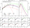 |
Fig. 3. Type Ia SN rate RIa as a function of redshift z (lower horizontal axis) and age (upper horizontal axis) assuming the CSFR of Madau & Dickinson (2014). Black markers represent the binned observational data compiled from the literature and reported in Table 1. The curves correspond to the best fits assuming the DTDs used in Palicio et al. (2023), while the black dashed-dotted line denotes a combination of the MR01 and G05Wide DTDs (see Sect. 5.2), both labeled in the legend. Upper right panel shows a zoomed-out view of the upper left one, enclosed by the dashed black lines. Bottom panels illustrate the confidence intervals (±1σ) of the Type Ia SN rate computed from the errors in CSFR, assuming the DTDs indicated in each legend. |
In order to select the best DTD, we used a least-squares method to fit the data for each combination of CSFR and DTD, and then we evaluated its quality by performing a χ2-test with d.o.f. degrees of freedom, where d.o.f.=N − 1 for the literature DTDs, d.o.f.=N − 2 for the combination proposed in Sect. 5.2, and N is the number of observational data points (see Table 2). The errors involved in the χ2 estimator are the quadratic sum of the observational errors and those computed for RIaCOSM in Eq. (3). The latter depends on the free parameter we are trying to optimize (AIa), introducing a nonlinear dependence on this parameter and requiring an iterative approach to minimize χ2. Fortunately, this approach converges in a few iterations. For each combination of DTD and CSFR, we determine the fraction  that minimizes χ2(AIa) (middle columns in Table 2), in which we account for the asymmetry of the error bars by using the upper (lower) errors when the fit overestimates (sub-estimates) the observations. The error of
  is estimated from the width of the χ2(AIa) curve near
  (Fisher 1922).
Summary of fit parameters found for all the tested combinations of DTDs and CSFRs.
5.2. Optimal combination of DTDs
Among the three theoretical DTDs considered in this work, only the G05Close DTD does not satisfactorily reproduce the observations of Type Ia SN rates, as noted in Matteucci et al. (2009). On the contrary, both the MR01 and the G05Wide DTDs proposed for the SD and DD scenarios, respectively, provide good fits to the observations. Since these DTDs account for independent channels to produce Type Ia SNe, it is reasonable to estimate their individual contributions to the observed rates by testing multiple combinations of both. We parameterize such combinations by the fraction of MR01 DTD contribution, fMR01, and repeat the fitting procedure of the observed data performed before. As Fig. 4 shows, an improvement of the fit is obtained only when Type Ia SN rates are computed assuming the Kim et al. (2024) CSFR, while for the Madau & Dickinson (2014) and the Harikane et al. (2022) CSFR the MR01 alone leads to optimal results. For the Kim et al. (2024) CSFR, the minimum of χ2 is found at fMR01 = 0.34 ± 0.01 (i.e., 34% of MR01 and 66% of the G05Wide DTD), leading to a fit as good as that obtained with the empirical T08 DTD. This combined DTD is represented by the black dash-dotted lines in the corresponding figures.
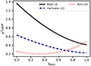 |
Fig. 4. Goodness of fit of the real data χ2 per degree of freedom (d.o.f.) as a function of the fraction of MR01 DTD (fMR01) included in the combination with the G05Wide DTD. The lines correspond to the CSFR labeled in the legend. |
If we consider the data only up to z = 1.5, which show smaller error bars, we can conclude that the best DTDs are those from MR01, T08, and G05Wide. In addition, we can completely exclude the S05 DTD, which assumes no prompt Type Ia SNe, and the G05Close DTDs as it underestimates (overestimates) the observations at redshifts lower (larger) than z ≈ 0.7. This situation is reversed when the P08 DTD is considered.
The same conclusions concerning those DTDs were reached by Matteucci et al. (2009), who studied the effects of different Type Ia SN DTDs on the chemical evolution of the Milky Way and concluded that the best DTDs are the SD and DD (wide) ones. It should be noted that T08 is an empirical DTD and is similar to G05Wide, so we do not consider it in the following.
As the left panels in Figs. 3, A.1, and A.2 illustrate, the discrepancies among the Type Ia SN rates computed for different DTDs become more evident at high redshifts, where the dependence on the cosmic SFR is also stronger. If we also include this regime in the comparison, in which the error bars of the observed Type Ia SN data are larger, then only the P08, S05, and G05Close DTDs can be firmly excluded.
These results confirm that the classical Type Ia SN scenarios (DD and SD) are the best to reproduce either the abundance patterns, for example, the plot [α/Fe] versus [Fe/H], or the cosmic Type Ia SN rate. This means that the fraction of prompt Type Ia SNe (i.e., all the SNe exploding in the first 100 Myr after star formation) should not exceed 15–20% of all Type Ia SNe, as it is evident from Fig. 1. Moreover, as already stated in previous papers (e.g., Matteucci et al. 2009; Palicio et al. 2023) the differences between the SD scenario of MR01 and the wide DD scenario of G05 are negligible from the point of view of the cosmic rate as well as of the galactic chemical evolution.
Concerning the adopted CSFRs, there is not much difference in the predicted cosmic Type Ia rates except for two cases: (i) when the CSFR of Harikane et al. (2022) is considered, the S05 DTD could be acceptable at low redshift, although it must be excluded anyway at high z due to the large discrepancy with the data; (ii) under the assumption of the Kim et al. (2024) CSFR, the T08 provides the optimal fit of the observed Type Ia SN rate. Although Hachisu et al. (2008) proved that the SD scenario can lead to such a form of DTD, the t−1 trend of the T08 DTD has been historically considered supportive of the DD scenario (see review by Maoz & Mannucci 2012). For instance, G05Wide and T08 have similar slopes in Fig. 1. This connection is further reinforced by the improvement in the data fit provided by the G05Wide DTD, which is proposed for the DD scenario, when the Kim et al. (2024) CSFR is considered. Using a smoothed version of a T08-like DTD, Childress et al. (2014) were able to fit a subset of our observed Type Ia SN rates both assuming the Behroozi et al. (2013) CSFR and that inferred from their mass assembly model.
In contrast with T08 and G05Wide, the MVP06 DTD constitutes the second preferential delay-time distribution when the SD channel dominates; that is, when the M&D14 and H22 CSFRs are assumed. This clearly supports the need for two explosion regimes that account for the “young” and “old” progenitors, respectively (Mannucci et al. 2005; Scannapieco & Bildsten 2005, the so-called A+B model), especially for modeling the Type Ia SN rates observed in early-type galaxies.
We compared our results with existing literature. Graur et al. (2014) explored two families of delay-time distributions – a power law and a Gaussian DTD – to determine which one leads to the optimal fit for an observational cosmic Type Ia SN rate dataset, keeping the parameters of the mentioned DTD as free variables (i.e., the slope of the power law, the median and width of the Gaussian, and the amplitudes of both). For all considered cosmic star-formation rates, the resulting slopes of the power-law DTD were approximately –1, which made them compatible with the T08 DTD. However, the Gaussian DTD failed to reproduce the observations at a 95% confidence level when the Behroozi et al. (2013) CSFR (their most similar CSFR to the M&D14 CSFR tested in this work) was considered.
Additionally, Graur et al. (2014) tested literature DTDs for both the SD and DD scenarios and concluded that the former leads to poor fits of the observed Type Ia SN rate. Even though a direct comparison with our results is not possible due to a different set of DTDs, we noted that their tests with the Yungelson (2010) DD DTD (similar to the T08 DTD) and Mennekens et al. (2010) DD DTD (similar to our “mix” DTD) provided visually satisfactory fits of their data points (see their Figures 13 and 14). On the contrary, their DTDs for the SD scenario show very different late-regime slopes and minimum delay times compared to the MR01 DTD used in our work. This might explain why we obtained opposite conclusions regarding the SD scenario.
More recently, Strolger et al. (2020) proposed a family of DTDs based on the skew-normal distribution (O’Hagan & Leonard 1976; Azzalini 1985, 2005) to fit a compendium of Type Ia SN rates (see their Table 5), while they considered a CSFR similar to that of Madau & Dickinson (2014) within ∼1σ. As a result, their best fit suggested an exponential-like DTD that approximates the t−1 T08 delay-time distribution, typically associated with the DD scenario (see discussion above).
Assuming the cosmic star-formation rate from Behroozi et al. (2013), Rodney et al. (2014) tested a piecewise DTD characterized by two well-defined regimes: a plateau extending from a minimum delay of 40 Myr (Belczynski et al. 2005) to an abrupt transition at t = 0.5 Gyr, followed by a t−1 power law at later times (t > 0.5 Gyr). The relative contribution of the prompt regime to the whole DTD is parameterized by the variable fp. Rodney et al. (2014) found fp ranges from 0.21 to 0.59 when considering only HST (CANDELS+CLASH Grogin et al. 2011; Koekemoer et al. 2011; Postman et al. 2012) and ground-based observations, respectively. Interestingly, the rough mean of these fp values provides a good approximation of our “mix” DTD for t ≳ 0.2 Gyr. When both HST and ground-based observations are combined, they obtain a fraction of fp ≈ 0.53, which is similar to that found by Mannucci et al. (2006).
Based on the results presented in this work, the SD and DD dichotomy is strongly dependent on the assumed CSFR. On one hand, those proposed by Madau & Dickinson (2014) and Harikane et al. (2022) suggest a cosmic Type Ia SN rate dominated by the SD scenario, without invoking a degenerate companion. On the contrary, when considering the Kim et al. (2024) CSFR, we need at least ∼65% of the total Type Ia SNe to be produced through the DD channel to explain the observations. However, as the authors point out, the CSFR proposed by Kim et al. (2024) flattens at z ≳ 6, diverging significantly from other CSFR models in the literature. The obtained contribution of 34% from SD progenitors to the total Type Ia SNe is of a similar order of magnitude to that proposed by Sternberg et al. (2011) for spirals (20–25%), as well as to that inferred by Meng et al. (2009) for the SD WD+main-sequence star mechanism (30%). However, it should be noted that the remaining 70% might include other SD scenarios (e.g., WD+red giant, WD+helium star) as well as the DD channel.
6. Conclusions and future perspectives
In this work, we evaluated multiple combinations of delay-time distributions and cosmic star-formation rates to model a compilation of Type Ia SN rates reported in the literature. For the cosmic star-formation rates, we made use of the expressions proposed by Madau & Dickinson (2014), Harikane et al. (2022), and Kim et al. (2024), while for the DTDs we considered those explored in Palicio et al. (2023), including the theoretical formulations for the SD and DD channels from Matteucci & Recchi (2001) and Greggio (2005), respectively, and the empirical ones from other works. Using a least-squares fitting technique, we determined the optimal fraction of Type Ia SN progenitors,  , for each combination of CSFRs and DTDs, whose goodness of fit is quantified by the p value of the associated χ2 test. We found that when the Madau & Dickinson (2014) and Harikane et al. (2022) CSFRs are considered, the MR01 DTD proposed for the SD scenario provides the best modeling for the observed Type Ia SN rates. For the case of the Kim et al. (2024) CSFR, however, the empirical delay-time distribution suggested by Totani et al. (2008) leads to the optimal fit of the observations. Though not optimal, the G05Wide DTD proposed by Greggio (2005) constitutes a good alternative to the T08 DTD for the latter CSFR. If we relax the criteria for a good fit to 1 − p > 0.95 (values highlighted in bold in Table 2), then only the MR01 DTD provides satisfactory fits for all the CSFRs (also the MVP06 DTD if we consider the results in Table C.1). However, for the H22 and K24 CSFRs, we cannot resolve the SD/DD degeneracy.
Finally, by combining the theoretic DTDs proposed for the SD and DD scenarios, we found the MR01 DTD alone is the best to reproduce the observed Type Ia SN rates in two of the three tested CSFRs (Madau & Dickinson 2014 and Harikane et al. 2022), while it requires 70% of the G05Wide to provide better results when the Kim et al. (2024) CSFR is considered. This dichotomy in the best scenario determination seems to be motivated by the different trend of the Kim et al. (2024) CSFR at high z when compared to the other CSFRs. The observations at a higher redshift allowed us to break the degeneracy noted by Bonaparte et al. (2013) in the determination of the dominant channel for the Type Ia SNe, giving preference to the SD scenario, although it was strongly dependent on the CSFR assumption.
In conclusion, our results prove that, even in the most favorable scenario for the DD channel, at least ∼34% of the observed Type Ia SNe must be produced by a WD with a nondegenerate companion. This implies the SD channel constitutes a viable scenario that should not be obviated (Livio 2000), offering an alternative mechanism to the sub-Chandra Type Ia-producing mergers, which were proposed to account for the limited number of close WD binaries capable of producing Type Ia SNe within the Hubble time (Maoz 2008; Mennekens et al. 2010). However, our results clearly show that other proposed Type Ia SN scenarios do not reproduce the cosmic Type Ia SN rate, irrespectively of the assumed CSFR, or the [α/Fe] versus [Fe/H] relation in the Milky Way (Matteucci et al. 2009). In the future, JWST (Gardner et al. 2006; Rigby et al. 2023) will hopefully provide more data of SNe Ia at high z, allowing us to anchor the predicted SN rates at earlier times, where the effect of the adopted DTD is more evident.
This critical value corresponds to the maximum accretion rate that allows stable hydrogen burning on the surface of the WD.
More precisely, the PTF 11kx SN is explained by the violent prompt merger mechanism, a sub-case of the CD scenario in which the Type Ia SN is produced shortly after the merger within the common envelope.
Acknowledgments
We thank the anonymous referee whose comments and corrections improved this manuscript. P. A. Palicio acknowledges the financial support from the Centre national d’ études spatiales (CNES). This work was partially supported by the European Union (ChETEC-INFRA, project no. 101008324). F. Matteucci thanks I.N.A.F. for the 1.05.12.06.05 Theory Grant - Galactic archaeology with radioactive and stable nuclei.
References
- Altavilla, G., Fiorentino, G., Marconi, M., et al. 2004, MNRAS, 349, 1344 [Google Scholar]
- Astier, P., Guy, J., Regnault, N., et al. 2006, A&A, 447, 31 [NASA ADS] [CrossRef] [EDP Sciences] [Google Scholar]
- Azzalini, A. 1985, Scand. J. Stat., 12, 171 [Google Scholar]
- Azzalini, A. 2005, Scand. J. Stat., 32, 159 [CrossRef] [Google Scholar]
- Barbary, K., Aldering, G., Amanullah, R., et al. 2012, ApJ, 745, 31 [NASA ADS] [CrossRef] [Google Scholar]
- Barris, B. J., & Tonry, J. L. 2006, ApJ, 637, 427 [CrossRef] [Google Scholar]
- Behroozi, P. S., Wechsler, R. H., & Conroy, C. 2013, ApJ, 770, 57 [NASA ADS] [CrossRef] [Google Scholar]
- Belczynski, K., Bulik, T., & Ruiter, A. J. 2005, ApJ, 629, 915 [Google Scholar]
- Betoule, M., Kessler, R., Guy, J., et al. 2014, A&A, 568, A22 [NASA ADS] [CrossRef] [EDP Sciences] [Google Scholar]
- Blanc, G., Afonso, C., Alard, C., et al. 2004, A&A, 423, 881 [NASA ADS] [CrossRef] [EDP Sciences] [Google Scholar]
- Bonaparte, I., Matteucci, F., Recchi, S., et al. 2013, MNRAS, 435, 2460 [NASA ADS] [CrossRef] [Google Scholar]
- Botticella, M. T., Riello, M., Cappellaro, E., et al. 2008, A&A, 479, 49 [NASA ADS] [CrossRef] [EDP Sciences] [Google Scholar]
- Cappellaro, E., Evans, R., & Turatto, M. 1999, A&A, 351, 459 [NASA ADS] [Google Scholar]
- Cappellaro, E., Botticella, M. T., Pignata, G., et al. 2015, A&A, 584, A62 [NASA ADS] [CrossRef] [EDP Sciences] [Google Scholar]
- Cenko, S. B., Li, W., Filippenko, A. V., et al. 2012, CBETs, 3014, 1 [Google Scholar]
- Childress, M. J., Wolf, C., & Zahid, H. J. 2014, MNRAS, 445, 1898 [Google Scholar]
- Chomiuk, L., Soderberg, A. M., Chevalier, R. A., et al. 2016, ApJ, 821, 119 [NASA ADS] [CrossRef] [Google Scholar]
- Dahlen, T., Strolger, L.-G., Riess, A. G., et al. 2004, ApJ, 613, 189 [NASA ADS] [CrossRef] [Google Scholar]
- Dahlen, T., Strolger, L.-G., & Riess, A. G. 2008, ApJ, 681, 462 [NASA ADS] [CrossRef] [Google Scholar]
- Darnley, M. J., Bode, M. F., Kerins, E., et al. 2006, MNRAS, 369, 257 [NASA ADS] [CrossRef] [Google Scholar]
- Darnley, M. J., Hounsell, R., O’Brien, T. J., et al. 2019, Nature, 565, 460 [NASA ADS] [CrossRef] [Google Scholar]
- Della Valle, M., & Izzo, L. 2020, A&ARv, 28, 3 [NASA ADS] [CrossRef] [Google Scholar]
- Della Valle, M., & Livio, M. 1996, ApJ, 473, 240 [NASA ADS] [CrossRef] [Google Scholar]
- Desai, D. D., Kochanek, C. S., Shappee, B. J., et al. 2024, MNRAS, 530, 5016 [NASA ADS] [CrossRef] [Google Scholar]
- Dhawan, S., Jha, S. W., & Leibundgut, B. 2018, A&A, 609, A72 [NASA ADS] [CrossRef] [EDP Sciences] [Google Scholar]
- Dilday, B., Kessler, R., Frieman, J. A., et al. 2008, ApJ, 682, 262 [Google Scholar]
- Dilday, B., Smith, M., Bassett, B., et al. 2010, ApJ, 713, 1026 [NASA ADS] [CrossRef] [Google Scholar]
- Dilday, B., Howell, D. A., Cenko, S. B., et al. 2012, Science, 337, 942 [NASA ADS] [CrossRef] [Google Scholar]
- Di Stefano, R. 2010, ApJ, 712, 728 [Google Scholar]
- Di Stefano, R., Voss, R., & Claeys, J. S. W. 2011, ApJ, 738, L1 [Google Scholar]
- El-Badry, K., & Rix, H.-W. 2018, MNRAS, 482, L139 [Google Scholar]
- Fisher, R. A. 1922, Philos. Trans. R. Soc. Lond. Ser. A, 222, 309 [NASA ADS] [Google Scholar]
- Frederiksen, T. F., Hjorth, J., Maund, J. R., et al. 2012, ApJ, 760, 125 [NASA ADS] [CrossRef] [Google Scholar]
- Frohmaier, C., Sullivan, M., Nugent, P. E., et al. 2019, MNRAS, 486, 2308 [CrossRef] [Google Scholar]
- Furusawa, H., Kosugi, G., Akiyama, M., et al. 2008, ApJS, 176, 1 [NASA ADS] [CrossRef] [Google Scholar]
- Galbany, L., Stanishev, V., Mourão, A. M., et al. 2016, A&A, 591, A48 [NASA ADS] [CrossRef] [EDP Sciences] [Google Scholar]
- Ganeshalingam, M., Li, W., & Filippenko, A. V. 2013, MNRAS, 433, 2240 [NASA ADS] [CrossRef] [Google Scholar]
- Gardner, J. P., Mather, J. C., Clampin, M., et al. 2006, Space Sci. Rev., 123, 485 [Google Scholar]
- Giavalisco, M., Ferguson, H. C., Koekemoer, A. M., et al. 2004, ApJ, 600, L93 [NASA ADS] [CrossRef] [Google Scholar]
- Gilfanov, M., & Bogdán, Á. 2010, Nature, 463, 924 [Google Scholar]
- Gioannini, L., Matteucci, F., & Calura, F. 2017, MNRAS, 471, 4615 [NASA ADS] [CrossRef] [Google Scholar]
- Graur, O., & Maoz, D. 2013, MNRAS, 430, 1746 [NASA ADS] [CrossRef] [Google Scholar]
- Graur, O., Poznanski, D., Maoz, D., et al. 2011, MNRAS, 417, 916 [Google Scholar]
- Graur, O., Rodney, S. A., Maoz, D., et al. 2014, ApJ, 783, 28 [NASA ADS] [CrossRef] [Google Scholar]
- Greggio, L. 2005, A&A, 441, 1055 [NASA ADS] [CrossRef] [EDP Sciences] [Google Scholar]
- Greggio, L., & Renzini, A. 1983, A&A, 118, 217 [NASA ADS] [Google Scholar]
- Greggio, L., Renzini, A., & Daddi, E. 2008, MNRAS, 388, 829 [NASA ADS] [CrossRef] [Google Scholar]
- Grogin, N. A., Kocevski, D. D., Faber, S. M., et al. 2011, ApJS, 197, 35 [NASA ADS] [CrossRef] [Google Scholar]
- Hachisu, I., Kato, M., & Nomoto, K. 1996, ApJ, 470, L97 [CrossRef] [Google Scholar]
- Hachisu, I., Kato, M., & Nomoto, K. 2008, ApJ, 683, L127 [CrossRef] [Google Scholar]
- Hamuy, M., Phillips, M. M., Maza, J., et al. 1995, AJ, 109, 1 [NASA ADS] [CrossRef] [Google Scholar]
- Hardin, D., Afonso, C., Alard, C., et al. 2000, A&A, 362, 419 [NASA ADS] [Google Scholar]
- Harikane, Y., Ono, Y., Ouchi, M., et al. 2022, ApJS, 259, 20 [NASA ADS] [CrossRef] [Google Scholar]
- Hillebrandt, W., Kromer, M., Röpke, F. K., & Ruiter, A. J. 2013, Front. Phys., 8, 116 [Google Scholar]
- Horesh, A., Kulkarni, S. R., Fox, D. B., et al. 2012, ApJ, 746, 21 [NASA ADS] [CrossRef] [Google Scholar]
- Hotokezaka, K., Nakar, E., Gottlieb, O., et al. 2019, Nat. Astron., 3, 940 [NASA ADS] [CrossRef] [Google Scholar]
- Iben, I., Jr., & Tutukov, A. V. 1994, ApJ, 431, 264 [NASA ADS] [CrossRef] [Google Scholar]
- Iglesias, C. A., & Rogers, F. J. 1991, ApJ, 371, L73 [NASA ADS] [CrossRef] [Google Scholar]
- Iglesias, C. A., & Rogers, F. J. 1993, ApJ, 412, 752 [Google Scholar]
- Iglesias, C. A., Rogers, F. J., & Wilson, B. G. 1987, ApJ, 322, L45 [NASA ADS] [CrossRef] [Google Scholar]
- Iglesias, C. A., Rogers, F. J., & Wilson, B. G. 1990, ApJ, 360, 221 [NASA ADS] [CrossRef] [Google Scholar]
- Ilkov, M., & Soker, N. 2012, MNRAS, 419, 1695 [NASA ADS] [CrossRef] [Google Scholar]
- Justham, S. 2011, ApJ, 730, L34 [NASA ADS] [CrossRef] [Google Scholar]
- Kashi, A., & Soker, N. 2011, MNRAS, 417, 1466 [NASA ADS] [CrossRef] [Google Scholar]
- Kato, M., & Hachisu, I. 2012, Bull. Astron. Soc. India, 40, 393 [NASA ADS] [Google Scholar]
- Kato, M., Saio, H., & Hachisu, I. 2015, ApJ, 808, 52 [Google Scholar]
- Khetan, N., Izzo, L., Branchesi, M., et al. 2021, A&A, 647, A72 [NASA ADS] [CrossRef] [EDP Sciences] [Google Scholar]
- Kim, S. J., Goto, T., Ling, C.-T., et al. 2024, MNRAS, 527, 5525 [Google Scholar]
- Klein, R. 2021, Res. Notes Am. Astron. Soc., 5, 39 [Google Scholar]
- Kobayashi, C., & Nomoto, K. 2009, ApJ, 707, 1466 [NASA ADS] [CrossRef] [Google Scholar]
- Kobayashi, C., Tsujimoto, T., Nomoto, K., Hachisu, I., & Kato, M. 1998, ApJ, 503, L155 [NASA ADS] [CrossRef] [Google Scholar]
- Koekemoer, A. M., Faber, S. M., Ferguson, H. C., et al. 2011, ApJS, 197, 36 [NASA ADS] [CrossRef] [Google Scholar]
- Kuznetsova, N., Barbary, K., Connolly, B., et al. 2008, ApJ, 673, 981 [NASA ADS] [CrossRef] [Google Scholar]
- Leonard, D. C. 2007, ApJ, 670, 1275 [NASA ADS] [CrossRef] [Google Scholar]
- Li, W., Bloom, J. S., Podsiadlowski, P., et al. 2011a, Nature, 480, 348 [NASA ADS] [CrossRef] [Google Scholar]
- Li, W., Chornock, R., Leaman, J., et al. 2011b, MNRAS, 412, 1473 [NASA ADS] [CrossRef] [Google Scholar]
- Livio, M. 2000, in Type Ia Supernovae, Theory and Cosmology, eds. J. C. Niemeyer, & J. W. Truran (Cambridge University Press), 33 [Google Scholar]
- Livio, M., & Mazzali, P. 2018, Phys. Rep., 736, 1 [Google Scholar]
- Madau, P., & Dickinson, M. 2014, ARA&A, 52, 415 [Google Scholar]
- Madau, P., Della Valle, M., & Panagia, N. 1998a, MNRAS, 297, L17 [CrossRef] [Google Scholar]
- Madau, P., Pozzetti, L., & Dickinson, M. 1998b, ApJ, 498, 106 [NASA ADS] [CrossRef] [Google Scholar]
- Madgwick, D. S., Hewett, P. C., Mortlock, D. J., & Wang, L. 2003, ApJ, 599, L33 [Google Scholar]
- Mannucci, F., Della Valle, M., Panagia, N., et al. 2005, A&A, 433, 807 [NASA ADS] [CrossRef] [EDP Sciences] [Google Scholar]
- Mannucci, F., Della Valle, M., & Panagia, N. 2006, MNRAS, 370, 773 [Google Scholar]
- Maoz, D. 2008, MNRAS, 384, 267 [CrossRef] [Google Scholar]
- Maoz, D., & Mannucci, F. 2012, PASA, 29, 447 [NASA ADS] [CrossRef] [Google Scholar]
- Maoz, D., Mannucci, F., & Nelemans, G. 2014, ARA&A, 52, 107 [Google Scholar]
- Matteucci, F. 2021, A&ARv, 29, 5 [NASA ADS] [CrossRef] [Google Scholar]
- Matteucci, F., & Greggio, L. 1986, A&A, 154, 279 [NASA ADS] [Google Scholar]
- Matteucci, F., & Recchi, S. 2001, ApJ, 558, 351 [NASA ADS] [CrossRef] [Google Scholar]
- Matteucci, F., Spitoni, E., Recchi, S., & Valiante, R. 2009, A&A, 501, 531 [NASA ADS] [CrossRef] [EDP Sciences] [Google Scholar]
- McCully, C., Jha, S. W., Foley, R. J., et al. 2014, Nature, 512, 54 [NASA ADS] [CrossRef] [Google Scholar]
- McCully, C., Jha, S. W., Scalzo, R. A., et al. 2022, ApJ, 925, 138 [NASA ADS] [CrossRef] [Google Scholar]
- Meng, X., & Han, Z. 2016, A&A, 588, A88 [NASA ADS] [CrossRef] [EDP Sciences] [Google Scholar]
- Meng, X., & Podsiadlowski, P. 2017, MNRAS, 469, 4763 [NASA ADS] [CrossRef] [Google Scholar]
- Meng, X., & Yang, W. 2012, A&A, 543, A137 [NASA ADS] [CrossRef] [EDP Sciences] [Google Scholar]
- Meng, X., Chen, X., & Han, Z. 2009, MNRAS, 395, 2103 [NASA ADS] [CrossRef] [Google Scholar]
- Meng, X. C., Li, Z. M., & Yang, W. M. 2011, PASJ, 63, 31 [Google Scholar]
- Melinder, J., Dahlen, T., Mencía Trinchant, L., et al. 2012, A&A, 545, A96 [NASA ADS] [CrossRef] [EDP Sciences] [Google Scholar]
- Mennekens, N., Vanbeveren, D., De Greve, J. P., & De Donder, E. 2010, A&A, 515, A89 [NASA ADS] [CrossRef] [EDP Sciences] [Google Scholar]
- Moe, M., Kratter, K. M., & Badenes, C. 2019, ApJ, 875, 61 [NASA ADS] [CrossRef] [Google Scholar]
- Neill, J. D., Sullivan, M., Balam, D., et al. 2006, AJ, 132, 1126 [Google Scholar]
- Neill, J. D., Hudson, M. J., & Conley, A. 2007, ApJ, 661, L123 [NASA ADS] [CrossRef] [Google Scholar]
- Nomoto, K. 1982a, ApJ, 253, 798 [Google Scholar]
- Nomoto, K. 1982b, ApJ, 257, 780 [Google Scholar]
- Nugent, P. E., Sullivan, M., Cenko, S. B., et al. 2011, Nature, 480, 344 [NASA ADS] [CrossRef] [Google Scholar]
- O’Hagan, A., & Leonard, T. 1976, Biometrika, 63, 201 [CrossRef] [MathSciNet] [Google Scholar]
- Okumura, J. E., Ihara, Y., Doi, M., et al. 2014, PASJ, 66, 49 [NASA ADS] [Google Scholar]
- Pain, R., Fabbro, S., Sullivan, M., et al. 2002, ApJ, 577, 120 [NASA ADS] [CrossRef] [Google Scholar]
- Palicio, P. A., Spitoni, E., Recio-Blanco, A., et al. 2023, A&A, 678, A61 [NASA ADS] [CrossRef] [EDP Sciences] [Google Scholar]
- Panagia, N., Van Dyk, S. D., Weiler, K. W., et al. 2006, ApJ, 646, 369 [NASA ADS] [CrossRef] [Google Scholar]
- Patat, F., Chandra, P., Chevalier, R., et al. 2007, Science, 317, 924 [NASA ADS] [CrossRef] [Google Scholar]
- Perlmutter, S., Aldering, G., della Valle, M., et al. 1998, Nature, 391, 51 [CrossRef] [Google Scholar]
- Perlmutter, S., Aldering, G., Goldhaber, G., et al. 1999a, ApJ, 517, 565 [Google Scholar]
- Perlmutter, S., Turner, M. S., & White, M. 1999b, Phys. Rev. Lett., 83, 670 [CrossRef] [Google Scholar]
- Perrett, K., Sullivan, M., Conley, A., et al. 2012, AJ, 144, 59 [NASA ADS] [CrossRef] [Google Scholar]
- Phillips, M. M. 1993, ApJ, 413, L105 [Google Scholar]
- Postman, M., Coe, D., Benítez, N., et al. 2012, ApJS, 199, 25 [Google Scholar]
- Poznanski, D., Maoz, D., Yasuda, N., et al. 2007, MNRAS, 382, 1169 [CrossRef] [Google Scholar]
- Pozzi, F., Calura, F., Gruppioni, C., et al. 2015, ApJ, 803, 35 [Google Scholar]
- Prieto, J. L., Chen, P., Dong, S., et al. 2020, ApJ, 889, 100 [Google Scholar]
- Pritchet, C. J., Howell, D. A., & Sullivan, M. 2008, ApJ, 683, L25 [NASA ADS] [CrossRef] [Google Scholar]
- Rest, A., Scolnic, D., Foley, R. J., et al. 2014, ApJ, 795, 44 [Google Scholar]
- Riess, A. G., Filippenko, A. V., Challis, P., et al. 1998, AJ, 116, 1009 [Google Scholar]
- Rigault, M., Copin, Y., Aldering, G., et al. 2013, A&A, 560, A66 [NASA ADS] [CrossRef] [EDP Sciences] [Google Scholar]
- Rigby, J., Perrin, M., McElwain, M., et al. 2023, PASP, 135, 048001 [NASA ADS] [CrossRef] [Google Scholar]
- Rodney, S. A., & Tonry, J. L. 2010, ApJ, 723, 47 [NASA ADS] [CrossRef] [Google Scholar]
- Rodney, S. A., Riess, A. G., Strolger, L.-G., et al. 2014, AJ, 148, 13 [Google Scholar]
- Rogers, F. J., & Iglesias, C. A. 1992, ApJS, 79, 507 [CrossRef] [Google Scholar]
- Ruiz-Lapuente, P. 2014, New Astron. Rev., 62, 15 [CrossRef] [Google Scholar]
- Ruiz-Lapuente, P. 2019, New Astron. Rev., 85, 101523 [CrossRef] [Google Scholar]
- Salpeter, E. E. 1955, ApJ, 121, 161 [Google Scholar]
- Scannapieco, E., & Bildsten, L. 2005, ApJ, 629, L85 [Google Scholar]
- Schmidt, B. P., Suntzeff, N. B., Phillips, M. M., et al. 1998, ApJ, 507, 46 [NASA ADS] [CrossRef] [Google Scholar]
- Shafter, A. W., Henze, M., Rector, T. A., et al. 2015, ApJS, 216, 34 [NASA ADS] [CrossRef] [Google Scholar]
- Soker, N. 2013, IAU Symp., 281, 72 [NASA ADS] [Google Scholar]
- Soker, N. 2024, Open J. Astrophys., 7, 31 [NASA ADS] [Google Scholar]
- Soker, N., Kashi, A., García-Berro, E., Torres, S., & Camacho, J. 2013, MNRAS, 431, 1541 [NASA ADS] [CrossRef] [Google Scholar]
- Soker, N., García-Berro, E., & Althaus, L. G. 2014, MNRAS, 437, L66 [Google Scholar]
- Starrfield, S., Bose, M., Iliadis, C., et al. 2020, ApJ, 895, 70 [NASA ADS] [CrossRef] [Google Scholar]
- Sternberg, A., Gal-Yam, A., Simon, J. D., et al. 2011, Science, 333, 856 [NASA ADS] [CrossRef] [Google Scholar]
- Strolger, L.-G., Riess, A. G., Dahlen, T., et al. 2004, ApJ, 613, 200 [Google Scholar]
- Strolger, L.-G., Riess, A. G., Dahlen, T., et al. 2005, ApJ, 635, 1370 [NASA ADS] [CrossRef] [Google Scholar]
- Strolger, L.-G., Rodney, S. A., Pacifici, C., Narayan, G., & Graur, O. 2020, ApJ, 890, 140 [NASA ADS] [CrossRef] [Google Scholar]
- Sullivan, M., Le Borgne, D., Pritchet, C. J., et al. 2006, ApJ, 648, 868 [NASA ADS] [CrossRef] [Google Scholar]
- Sullivan, M., Guy, J., Conley, A., et al. 2011, ApJ, 737, 102 [NASA ADS] [CrossRef] [Google Scholar]
- Suzuki, N., Rubin, D., Lidman, C., et al. 2012, ApJ, 746, 85 [NASA ADS] [CrossRef] [Google Scholar]
- Tonry, J. L., Schmidt, B. P., Barris, B., et al. 2003, ApJ, 594, 1 [NASA ADS] [CrossRef] [Google Scholar]
- Totani, T., Morokuma, T., Oda, T., Doi, M., & Yasuda, N. 2008, PASJ, 60, 1327 [NASA ADS] [CrossRef] [Google Scholar]
- Turatto, M., Cappellaro, E., & Benetti, S. 1994, AJ, 108, 202 [Google Scholar]
- Tutukov, A. V., & Iungelson, L. R. 1976, Astrofizika, 12, 521 [NASA ADS] [Google Scholar]
- Tutukov, A. V., & Yungelson, L. R. 1979, Acta Astron., 29, 665 [NASA ADS] [Google Scholar]
- Valiante, R., Matteucci, F., Recchi, S., & Calura, F. 2009, New Astron., 14, 638 [NASA ADS] [CrossRef] [Google Scholar]
- Wang, X., Wang, L., Filippenko, A. V., Zhang, T., & Zhao, X. 2013, Science, 340, 170 [NASA ADS] [CrossRef] [Google Scholar]
- Webbink, R. F. 1984, ApJ, 277, 355 [NASA ADS] [CrossRef] [Google Scholar]
- Wheeler, J. C., & Hansen, C. J. 1971, Ap&SS, 11, 373 [Google Scholar]
- Whelan, J., Iben, Icko J., 1973, ApJ, 186, 1007 [CrossRef] [Google Scholar]
- Williams, S. C., Darnley, M. J., Bode, M. F., & Shafter, A. W. 2016, ApJ, 817, 143 [NASA ADS] [CrossRef] [Google Scholar]
- Yungelson, L. R. 2010, Astron. Lett., 36, 780 [Google Scholar]
Appendix A: Additional figures
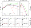 |
Fig. A.1. Same as Fig. 3, but for the CSFR of Harikane et al. (2022). |
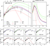 |
Fig. A.2. Same as Fig. 3, but for the CSFR of Kim et al. (2024). |
Appendix B: Table of individual Type Ia SN rates
Table with the individual measurements binned and averaged in Table 1.
Compilation of individual measurements of observed Type Ia SN rates.
Appendix C: Results with the individual measurements
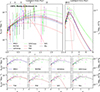 |
Fig. C.1. Type Ia SN rate RIa as function of redshift z (lower horizontal axis) and age (upper horizontal axis) assuming the CSFR of Madau & Dickinson (2014). Each marker-color pair corresponds to one reference in the literature: Li et al. 2011b (open red triangles); Neill et al. 2006 (filled blue stars); Barris & Tonry 2006 (open red pentagons); Graur & Maoz 2013 (filled blue hexagons); Madgwick et al. 2003 (filled magenta circles); Poznanski et al. 2007 (open black diamonds); Cappellaro et al. 1999 (filled red squares); Frohmaier et al. 2019 (open blue triangles); Barbary et al. 2012 (open red stars); Melinder et al. 2012 (filled cyan pentagons); Blanc et al. 2004 (filled red hexagons); Hardin et al. 2000 (filled red circles); Kuznetsova et al. 2008 (open magenta diamonds); Graur et al. 2014 (open lime squares); Perrett et al. 2012 (open black triangles); Dilday et al. 2010 (open lime stars); Rodney et al. 2014 (open black pentagons); Okumura et al. 2014 (open lime hexagons); Botticella et al. 2008 (filled cyan circles); Dahlen et al. 2004 (open lime diamonds); Rodney & Tonry 2010 (open black squares); Cappellaro et al. 2015 (open magenta triangles); Neill et al. 2007 (open blue stars); Graur et al. 2011 (filled magenta pentagons); Pain et al. 2002 (filled magenta hexagons); Dilday et al. 2008 (filled blue diamonds); Tonry et al. 2003 (open magenta squares); Dahlen et al. 2008 (open lime triangles); Desai et al. 2024 (solid black circle). The curves represent the best fits for the assumed DTDs (labeled in the legend). Upper right panel gives a zoomed-out version of the upper left one (enclosed by the dashed lines) without showing the error bars for the sake of visualization. Bottom panels illustrate the confidence intervals (±1σ) of the Type Ia SN rate computed from the errors in CSFR, assuming the DTDs indicated in each legend. |
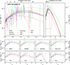 |
Fig. C.2. Same as Fig. C.1, but for the CSFR of Harikane et al. (2022). |
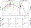 |
Fig. C.3. Same as Fig. C.1, but for the CSFR of Kim et al. (2024). |
Fit parameters found for all the tested combinations of DTDs and CSFRs, considering the measurements of RIa(z) of Table B.1.
All Tables
Summary of fit parameters found for all the tested combinations of DTDs and CSFRs.
Fit parameters found for all the tested combinations of DTDs and CSFRs, considering the measurements of RIa(z) of Table B.1.
All Figures
|
Fig. 1. Different DTD functions assumed in this work: Matteucci & Recchi (2001, solid blue curve); Mannucci et al. (2006, dotted green curve); wide and close from Greggio (2005, dashed blue and solid green curves, respectively); Totani et al. (2008, solid red curve); Pritchet et al. (2008, dashed red curve); and Strolger et al. (2005, dotted red curve). The optimal combination of DTDs detailed in Sect. 5.2 is denoted by the dotted-dashed black line. All the distributions are normalized by their maximum. |
| In the text | |
|
Fig. 2. Curves here represent adopted CSFRs derived by the best fit to observations as a function of redshift. The solid black line shows the CSFR of Madau & Dickinson (2014), the dashed blue line corresponds to the CSFR of Harikane et al. (2022), while the dotted red line represents the CSFR of Kim et al. (2024). |
| In the text | |
|
Fig. 3. Type Ia SN rate RIa as a function of redshift z (lower horizontal axis) and age (upper horizontal axis) assuming the CSFR of Madau & Dickinson (2014). Black markers represent the binned observational data compiled from the literature and reported in Table 1. The curves correspond to the best fits assuming the DTDs used in Palicio et al. (2023), while the black dashed-dotted line denotes a combination of the MR01 and G05Wide DTDs (see Sect. 5.2), both labeled in the legend. Upper right panel shows a zoomed-out view of the upper left one, enclosed by the dashed black lines. Bottom panels illustrate the confidence intervals (±1σ) of the Type Ia SN rate computed from the errors in CSFR, assuming the DTDs indicated in each legend. |
| In the text | |
|
Fig. 4. Goodness of fit of the real data χ2 per degree of freedom (d.o.f.) as a function of the fraction of MR01 DTD (fMR01) included in the combination with the G05Wide DTD. The lines correspond to the CSFR labeled in the legend. |
| In the text | |
|
Fig. A.1. Same as Fig. 3, but for the CSFR of Harikane et al. (2022). |
| In the text | |
|
Fig. A.2. Same as Fig. 3, but for the CSFR of Kim et al. (2024). |
| In the text | |
|
Fig. C.1. Type Ia SN rate RIa as function of redshift z (lower horizontal axis) and age (upper horizontal axis) assuming the CSFR of Madau & Dickinson (2014). Each marker-color pair corresponds to one reference in the literature: Li et al. 2011b (open red triangles); Neill et al. 2006 (filled blue stars); Barris & Tonry 2006 (open red pentagons); Graur & Maoz 2013 (filled blue hexagons); Madgwick et al. 2003 (filled magenta circles); Poznanski et al. 2007 (open black diamonds); Cappellaro et al. 1999 (filled red squares); Frohmaier et al. 2019 (open blue triangles); Barbary et al. 2012 (open red stars); Melinder et al. 2012 (filled cyan pentagons); Blanc et al. 2004 (filled red hexagons); Hardin et al. 2000 (filled red circles); Kuznetsova et al. 2008 (open magenta diamonds); Graur et al. 2014 (open lime squares); Perrett et al. 2012 (open black triangles); Dilday et al. 2010 (open lime stars); Rodney et al. 2014 (open black pentagons); Okumura et al. 2014 (open lime hexagons); Botticella et al. 2008 (filled cyan circles); Dahlen et al. 2004 (open lime diamonds); Rodney & Tonry 2010 (open black squares); Cappellaro et al. 2015 (open magenta triangles); Neill et al. 2007 (open blue stars); Graur et al. 2011 (filled magenta pentagons); Pain et al. 2002 (filled magenta hexagons); Dilday et al. 2008 (filled blue diamonds); Tonry et al. 2003 (open magenta squares); Dahlen et al. 2008 (open lime triangles); Desai et al. 2024 (solid black circle). The curves represent the best fits for the assumed DTDs (labeled in the legend). Upper right panel gives a zoomed-out version of the upper left one (enclosed by the dashed lines) without showing the error bars for the sake of visualization. Bottom panels illustrate the confidence intervals (±1σ) of the Type Ia SN rate computed from the errors in CSFR, assuming the DTDs indicated in each legend. |
| In the text | |
|
Fig. C.2. Same as Fig. C.1, but for the CSFR of Harikane et al. (2022). |
| In the text | |
|
Fig. C.3. Same as Fig. C.1, but for the CSFR of Kim et al. (2024). |
| In the text | |
Current usage metrics show cumulative count of Article Views (full-text article views including HTML views, PDF and ePub downloads, according to the available data) and Abstracts Views on Vision4Press platform.
Data correspond to usage on the plateform after 2015. The current usage metrics is available 48-96 hours after online publication and is updated daily on week days.
Initial download of the metrics may take a while.