| Issue |
A&A
Volume 698, June 2025
|
|
|---|---|---|
| Article Number | A48 | |
| Number of page(s) | 11 | |
| Section | Stellar structure and evolution | |
| DOI | https://doi.org/10.1051/0004-6361/202452341 | |
| Published online | 28 May 2025 | |
50 Dra: Am-type twins with additional variability in a non-eclipsing system
1
Astronomical Institute of the Czech Academy of Sciences, Fričova 298, CZ-25165 Ondřejov, Czech Republic
2
Institute of Theoretical Physics, Faculty of Mathematics and Physics, Charles University, V Holešovičkách 2, 180 00 Praha 8, Czech Republic
3
Instytut Astronomiczny, Uniwersytet Wrocławski, Kopernika 11, PL-51-622 Wrocław, Poland
4
Department of Theoretical Physics and Astrophysics, Masaryk University, Kotlářská 2, CZ-61137 Brno, Czech Republic
⋆ Corresponding author: This email address is being protected from spambots. You need JavaScript enabled to view it.
Received:
23
September
2024
Accepted:
8
April
2025
Abstract
Context. The interplay between radiative diffusion, rotation, convection, and magnetism in metallic-line chemically peculiar stars is not yet fully understood. Recently, evidence has emerged that these effects can work together.
Aims. Our goal was to study the bright binary system 50 Dra, describe its orbit and components, and study additional variability.
Methods. We conducted our analysis using TESS short-cadence data and new high-resolution spectroscopic observations. We disentangled the spectra using KOREL and performed spectral synthesis with ATLAS9 and SYNTHE codes. The system was modelled using KOREL and PHOEBE2.4. We also employed SED fitting in ARIADNE and isochrone fitting using PARAM1.5 codes.
Results.Our findings indicate that the non-eclipsing system 50 Dra (with an inclination of 49.9(8) deg), which displays ellipsoidal brightness variations, consists of two nearly equal A-type stars with masses of M1 = 2.08(8) and M2 = 1.97(8) M⊙, and temperatures of 9800(100) and 9200(200) K, respectively. Our analysis also indicates that the system, with an orbital period of Porb = 4.117719(2) days, is tidally relaxed with a circular orbit and synchronous rotation of the components. Furthermore, we discovered that both stars are metallic-line Am chemically peculiar stars with an underabundance of Sc and an overabundance of iron-peak and rare-earth elements. We identified additional variations with slightly higher frequency than the rotational frequency of the components that we interpret as prograde g-mode pulsations.
Conclusions. The system 50 Dra exhibits multiple co-existing phenomena and may have an impact on our understanding of chemical peculiarities and pulsations.
Key words: methods: data analysis / binaries: spectroscopic / stars: chemically peculiar / stars: rotation / stars: variables: general
© The Authors 2025
 Open Access article, published by EDP Sciences, under the terms of the Creative Commons Attribution License (https://creativecommons.org/licenses/by/4.0), which permits unrestricted use, distribution, and reproduction in any medium, provided the original work is properly cited.
This article is published in open access under the Subscribe to Open model. This email address is being protected from spambots. You need JavaScript enabled to view it. to support open access publication.
1. Introduction
About a third of spectral A-type stars show a deficiency of He, Ca, and/or Sc an overabundance of iron-group and rare-earths metals (Abt 1981; Gray et al. 2016). These stars, which are mostly observed in spectral types earlier than F2 within a typical temperature range between 7250 and 8250 K (Gray et al. 2016; Qin et al. 2019), are termed metallic-line chemically peculiar (CP) stars, or AmFm stars. Their peculiar chemical compositions arise from atomic diffusion, which occurs in stars with stable outer layers that transfer energy through radiation (Michaud 1970). This condition is satisfied in slowly rotating stars (< ≃ 100 km s−1) where rotational mixing is weak (Abt & Morrell 1995; Qin et al. 2021; Trust et al. 2020). It is not surprising that more than 70 % of AmFm stars are found in binary systems, particularly those with orbital periods shorter than 20 days (peaking around 5 days), where tidal effects slow the stars’ rotation rates (Abt 1961; Abt & Levy 1985; Carquillat & Prieur 2007). Systems where both components are AmFm-type appear common, as evidenced by Catanzaro et al. (2024), who studied six eclipsing binaries with AmFm stars and found that four of these systems exhibit the AmFm peculiarity in both primary and secondary components.
Although He is expected to rapidly gravitationally settle in AmFm stars (Charbonneau & Michaud 1991), they were not expected to pulsate. However, Am stars exhibiting p-mode pulsations were documented prior to the availability of ultra-precise space data (Kurtz 1989). Current observations confirm that AmFm stars can pulsate as δ Sct, γ Dor, and hybrid pulsators (e.g. Balona et al. 2015; Smalley et al. 2017; Dürfeldt-Pedros et al. 2024). It was also discovered that insufficient He in the He II ionisation zone leads to pressure modes in δ Sct AmFm stars being excited either by the turbulent pressure mechanism in the hydrogen ionisation zone (Antoci et al. 2014; Smalley et al. 2017) or by a bump in the Rosseland mean opacity resulting from the discontinuous H-ionisation edge in bound-free opacity (Murphy et al. 2020).
It is generally assumed that rotationally induced variability can only be observed in CP stars with strong (kG), globally-organised magnetic fields that can stabilise abundance spots (Ap/Bp stars, Preston 1974). However, a recent investigation of an Ap star 45 Her with a magnetic field strength of only 100 G by Kochukhov et al. (2023) questioned the necessity of strong magnetic fields to stabilise spots. Furthermore, precise space observations revealed that CP stars without strong magnetic fields (HgMn and AmFm stars) and normal A-type stars also show rotation modulation (e.g. Balona 2011; Sikora et al. 2019; Kochukhov et al. 2021; Trust et al. 2020). The brightness variations in the non-magnetic A-stars are less regular than in magnetic CP stars and resemble the differential rotation and spot evolution observed in cool stars (e.g. Balona 2011; Blazère et al. 2020). This observational evidence, combined with the spot evolution in some HgMn stars (Kochukhov et al. 2007) and rotation periods of less than 1 day observed in some Am stars (Trust et al. 2020), challenges the requirement for stable and calm atmospheres in these stars1.
The Fourier spectrum of many normal and AmFm stars shows a broad group of closely spaced peaks, often with a single peak or a very narrow group of unresolved peaks (Balona 2013; Balona et al. 2015; Trust et al. 2020; Henriksen et al. 2023a). Recent studies attribute the sharp peak (referred to as the ‘spike’) to surface rotational modulation connected with stellar spots and complex magnetic fields generated in the sub-surface convective layer (Antoci et al. 2025). The broad group of peaks (the ‘hump’) likely arises from either prograde g-modes (spike at lower frequency) or unresolved Rossby modes (spike at higher frequency). The Rossby modes are mechanically excited by deviated flows caused by stellar spots, mass outbursts, and by non-synchronous tidal forces (Saio et al. 2018).
Our study focuses on a 5.3-mag star, 50 Dra (basic parameters in Table 1), a double-line spectroscopic binary system. The binary nature of 50 Dra was first discovered by Harper (1919), who found an orbital period of 4.1175 days and estimated the basic parameters of the orbit. Skarka et al. (2022) classified this star as a ROTM|GDOR variable, suggesting variations connected with rotation and/or pulsations. We collected new spectroscopic observations over a century later and found almost the same orbital parameters as Harper (1919). However, combining our new spectroscopic observations with photometric data from the Transiting Exoplanet Survey Satellite (TESS) mission (Sect. 2, Ricker et al. 2015) revealed ellipsoidal and additional brightness variations (Sect. 3). This enabled us to determine the parameters of the system and both components (Sect. 4), and to identify both stars as metallic-line CP stars (Sect. 5). All features of 50 Dra are discussed in Sect. 6.
Basic characteristics of 50 Dra.
2. Observations
2.1. TESS photometry
We collected available data reduced by the TESS Science Processing Operations Centre (SPOC; Jenkins et al. 2016) and the Quick-Look Pipeline (QLP; Huang et al. 2020a,b) using LIGHTKURVE software (Lightkurve Collaboration 2018; Barentsen & Lightkurve Collaboration 2020) from the Mikulski Archive for Space Telescopes (MAST) archive. We extracted the pre-search data conditioning simple aperture photometry (PDCSAP) flux with long-term trends removed (Twicken et al. 2010) and transformed the normalised flux to magnitudes. The LIGHTKURVE software was also used to stitch data from different sectors together.
Data generated by various pipelines at varying cadences exhibit differences. The most reliable products are the 2-min short-cadence (SC) data sets from the Science Processing Operations Center (SPOC), as discussed by Skarka et al. (2022). The distinctions between the 50 Dra data products are illustrated in Fig. 1. The frequency spectra of the SPOC SC data exhibit the lowest noise levels and lack the artificial peak at 0.07 c/d (as seen in the QLP data). The distribution of SC data decreases the presence of artificial data peaks, such as those around the dominant frequency peak at 0.48 c/d. Consequently, we based our analysis on the 2-minute SPOC data. We acquired SPOC SC data from 28 sectors (14–26, 40–41, 47–58, 60, and 74), excluding data from Sector 25 due to its poor quality. We used a total of 440 166 observations at 2-min cadence, spanning almost 4.5 years (1629 days, from 2019–2024).
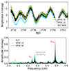 |
Fig. 1. Comparison of the available data products generated by different pipelines (top panel) and corresponding frequency spectra with labelled features (bottom panel). |
The contamination ratio of only 0.02% (Paegert et al. 2021) suggests no contamination of the 50 Dra light. The only possible contaminants are two bright stars located 20 and 34 arcmin away2 and 17 additional faint stars (7.7–12.5 mag fainter than 50 Dra, see Table A.1) near 50 Dra, shown in Fig. 2. However, the two bright stars do not show signatures of variability similar to 50 Dra, and a custom aperture analysis around the faint, numbered stars in Fig. 2 rules out the possibility that any of the signals observed in 50 Dra originates from a different star.
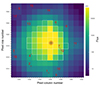 |
Fig. 2. Vicinity of 50 Dra showing the aperture mask in Sector 14 with identification of possible contaminants identified in Table A.1. The field size shown in the figure is approximately 4 × 4 arcmin. |
2.2. Spectroscopy
We obtained 20 spectra of 50 Dra between February and July 2022 using the Ondřejov Echelle Spectrograph (OES) at the 2m Perek telescope (Ondřejov, Czech Republic). The spectrograph has a resolving power of R = λ/δλ≈50 000 in the Hα region and covers a spectral range of 3800–9100 Å (Koubský et al. 2004; Kabáth et al. 2020). The spectra were processed and reduced using standard tasks in the IRAF package (Tody 1986), and cosmic-particle hits were eliminated using the DCR code (Pych 2004). The median S/N of the 600-second exposures in the Hα region was 150, with only four exposures having S/N slightly less than 100, and a few reaching S/N = 230.
3. Photometric variability
We observed the expected double-wave variations in the TESS SC light curve, with a period of Porb = 4.117719(2) days (peaks labelled forb in Fig. 1). This period agrees with the orbital period derived from spectroscopic observations but is more precise due to the extended time span. As expected, a primary minimum occurs at the inferior conjunction of the binary components.
Given the short orbital period and the almost perfectly sinusoidal radial velocity (RV) curves of both components (within observational uncertainties) it is reasonable to assume that the trajectory of the binary star’s components is nearly circular (see Sect. 4, Table 3 and Fig. 7). As a result, the light curve of this non-eclipsing binary, Fell(t), can be well approximated by a simple trigonometric polynomial model:
 (1)
(1)
where t is the BJD timestamp and M0 is the reference time for the start of the phase that we set at the moment of the inferior conjunction (the time of the deeper minimum). The phase function (ϑ(t)) is the sum of the number of orbits completed by the system since the passage through the basic inferior conjunction and the fractional orbital phase φ = Frac(ϑ). The coefficients of the model are denoted as A1, A2, A3, A4, and  . The binned data along with the model are shown in Fig. 3.
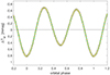 |
Fig. 3. TESS SC data of 50 Dra phase-folded with the orbital period. Each circle corresponds to the mean of 4400 individual TESS observations. |
Symmetrical terms of the ellipsoidal variability correspond to the effects of tidal deformation and reflection, while the anti-symmetrical term, which causes the uneven heights of maxima, results from Doppler beaming (e.g. Zucker et al. 2007). The parameters of the model with Eq. (1) are in Table 2.
Model parameters of the ellipsoidal variations.
After removing variability related to the orbital period Porb = 4.117719 days, a complex, unresolved variability around 0.27 and 0.55 c/d persists in the frequency spectrum (see Fig. 1 and 4). Since the group of peaks with higher frequencies is in the region of harmonics and combination peaks of the lower frequencies, we assume that the peaks have a common nature. As shown in Fig. 4, which shows the frequency spectra of approximately 100-day segments, the variation changes over time. We discuss possible explanations for this additional variability in Sect. 6. Apart from the ellipsoidal variability peaks and the unresolved peaks around 0.27 and 0.55 c/d, we did not find any other significant frequencies.
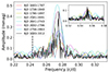 |
Fig. 4. Frequency spectrum centred around a group of peaks produced by additional variability from different data segments (coloured lines) and the full data set (black line). The amplitude of the frequency spectrum of the full dataset is multiplied by two for better readability. The black dashed line denotes the position of the orbital and rotational frequency. |
4. System parameters
4.1. Spectral energy distribution
We used photometry across 12 filters spanning visual to infra-red wavelengths (Table A.2) and fitted the spectral energy distribution (SED) with ARIADNE (Vines & Jenkins 2022). This code uses SED fitting methods and Gaia distances. It then combines results via Bayesian model averaging to derive basic stellar parameters such as Teff, log g, iron abundance [Fe/H], extinction, and stellar radius.
The SED fitting results are shown in Fig. 5, with derived values listed in Table 1 (labelled ‘SED’ in the column ‘Source’). The results are provided for reference only, since 50 Dra is not a single star. However, this exercise illustrates the reliability of the literature-derived stellar parameters when considering 50 Dra as a single object. The temperature Teff = 9123 K, [Fe/H] = –0.07 dex, and log g = 3.90 are within uncertainties with the catalogue values, particularly the excellent agreement in Teff with the value of Paegert et al. (2021). The largest discrepancy is in the iron abundance, which is around 0.3 dex lower than the [Fe / H] values from Gaia Collaboration (2023) and from our spectroscopic analysis (see Sect. 4). Thus, the [Fe/H] form of the SED is less reliable than that of other methods. We adopt the radius R* = 2.91(9) R⊙, derived using ARIADNE under the single star assumption, to derive the radii of the components in Sect. 4.4. This is possible because, as demonstrated by the spectral synthesis (see Sect. 5) the stars have similar temperatures (in the range 9000 − 10 000 K). This results in their SEDs being nearly scaled versions of each other in the visual and infrared bands used to derive R*, with a better approximation at longer wavelengths. We note that binary SED fitting alone fails to converge to a well-defined solution, even using the priors on temperature from spectra, due to degeneracies between the component radii. In case of equal temperatures, we obtain only the constraint R*2 = R12 + R22.
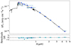 |
Fig. 5. Spectral energy distribution (SED) derived from photometric observations (Table A.2) using ARIADNE. |
4.2. Spectra disentanglement
Since 50 Dra is a double-lined spectroscopic binary (SB2) system, variations in the spectral line positions of both components are distinct and apparent at first glance (see Fig. 6). The movement of some of the prominent spectral lines during orbital motion is best demonstrated by the trail plots in the lower panel of Fig. 6. We performed Fourier spectral disentangling using the KOREL code (Hadrava 1995, 2004), which performs simultaneous decomposition of spectra and solution of orbital parameters. We fixed the orbital period P = 4.117719 days, as it was precisely determined from ellipsoidal variations in photometric data spanning almost 4.5 years (Sect. 3).
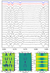 |
Fig. 6. Top: Observed spectra in different orbital phases around the Mg I 5167–5183 Å triplet and Fe II 5169 Å lines. The mean disentangled spectra for the primary and secondary components are shown in blue and red, respectively. Bottom: Trails of Na D, Si II, and Hα lines (from left to right) showing the variation of the position of the lines of both components during the orbital cycle. The relative intensity of the lines is also indicated. |
We performed the Fourier spectral disentangling in 41 spectral regions with a typical width of 140 Å. An example of the final disentangled spectra of both components around the Mg I 5167–5183 Å triplet is shown in the upper panel of Fig. 6. KOREL also derives RVs and provides a model of the orbit (see Sect. 4.3 and Table 3). To ensure consistency, we retained only 25 spectral regions with a sufficient number of spectral lines. The RV values for both components are listed in Table A.3 together with their errors, calculated as the standard deviation of the values from the individual segments.
Parameters of the binary system.
4.3. Orbital parameters
We determined the orbital parameters (time of periastron passage T0, eccentricity e, argument of pericentre ω, semi-amplitudes of radial velocities K1, K2, and mass ratio q = M2/M1) using KOREL’S disentangling process, solving the orbit simultaneously across all disentangled regions. The values in Table 3, which are calculated as the average values of all solutions in 25 spectral regions, indicate a circular orbit (e is almost zero) with large semi-amplitudes of the RV curves (K1 ≈ 79 km s−1, K2 ≈ 83 km s−1). The similarity in semi-amplitudes, and thus the mass ratio q ≈ 0.95, show that both components have almost equal masses (see Fig. 7). Systems with q ≃ 1 components are commonly observed among AmFm binaries, consistent with the findings of Carquillat & Prieur (2007), who found that six out of 12 of their SB2 systems had q > 0.9. Notably, all of our values are consistent with those estimated over a century ago by Harper (1919).
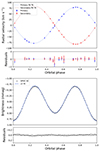 |
Fig. 7. Radial velocity curve of both components with the best fit (upper panel) and the light curve with the best fit (bottom panel). The photometric points are binned to produce 500 points per orbital phase. |
The only discrepancy between our results and the values in the literature is the systemic velocity γ, where our value (γ = −6.53(9) km s−1) is about 1-2 km s−1 higher than previous estimates (see Table 1). We did not identify any problem in our analysis that could explain the difference. Since all of the previous values are based on low-resolution spectroscopy and/or historical photographic plates, we assume that our new value is more reliable than those published previously.
4.4. Characteristics of the system components
To estimate stellar parameters, we used the Bayesian fitting tool PARAM 1.53 (da Silva et al. 2006; Rodrigues et al. 2014, 2017). The code uses a new version of PARSEC (Bressan et al. 2012) evolutionary tracks and isochrones that include the effects of rotation, improvements in nuclear reaction networks, and other effects (Nguyen et al. 2022). Since 50 Dra is not a single star, we derived individual observed magnitudes for each component.
If we assume the mass ratio q ≈ 0.951 and the mass-luminosity relation L ≃ M4.329 for the main-sequence stars in the 1.05–2.4 M⊙ range (based on 275 well measured stars, Eker et al. 2018), we derive the flux ratio FPrim/FSec = 0.951−4.329 = 1.243. After transformation into magnitudes, we obtain VPrim = 5.997 mag and VSec = 6.238 mag by assuming the total magnitude of the system is VT = 5.358 mag (Høg et al. 2000). We used the calculated V magnitudes, Teff, log g, and [Fe/H] from Table 4, and the Gaia DR3 parallax from Table 1 as input parameters for PARAM 1.5. Although these are only rough estimates, the resulting values (see Table 3) are all within errors consistent with results from binary star modelling and spectral analysis (Sect. 5).
Parameters of the components and their abundances from the spectral synthesis.
As an alternative and more appropriate way to derive system parameters without using stellar evolution models, we used the light-curve model, the SED fit, and the radial velocities. We used PHOEBE 2.4 (Conroy et al. 2020) to run the binary model. Since Doppler beaming, apparent in our light curve, is not currently implemented in PHOEBE 2.4, and the use of SED is quite convoluted, we directly computed radii and temperatures.
The Doppler beaming amplitude ΔF is given by
 (2)
(2)
where c is the speed of light and β1, β2 are Doppler beaming coefficients of the stars. The relative beaming amplitude,  , taken with respect to the total flux of the binary components, F = F1 + F2, can easily be converted from the magnitude value A4 in Table 2 corresponding to the expansion in Eq. (1). Using the radial velocity amplitudes K1 and K2 from Sect. 4.3 and beaming coefficients β1 = 2.01(5) and β2 = 2.09(5), derived by interpolation of tables by Claret et al. (2020) for the TESS passband, we get the passband relative fluxes F1/(F1 + F2) = 0.547(9) and F2/(F1 + F2) = 0.453(9). Next, we used PHOEBE to derive the relation between the flux and temperature ratios for stars with the same radius R1 = R2 = 2 R⊙ in the TESS passband. Using the range T2/T1 ∈ (0.90, 1.00) and the primary star temperature T1 = 9800 K we derive a linear relation between the two. After incorporating the surface area ratio, we obtain the final relation:
 (3)
(3)
To obtain the radii themselves, we used the SED result for R*. In the long wavelength limit (far IR) under the Rayleigh-Jeans approximation it should hold
 (4)
(4)
where R*, and T* are the stellar radius and effective temperature derived under the single star assumption in Sect. 4.1. Using the effective temperatures of stars T1 = 9800(100) K and T2 = 9200(200) K derived from spectra (see Sect. 5) we get the radii R1 = 2.06(9) and R2 = 1.99(9).
Next, we fit the ellipsoidal variation using PHOEBE to determine the inclination of the system. We used PHOENIX atmospheric models by Husser et al. (2013) to obtain passband luminosities and limb-darkening coefficients. We set bolometric gravity brightening coefficients of both stars b1 = b2 = 1.0 and bolometric reflection coefficients to a1 = a2 = 1.0, valid for stars with radiative atmospheres above T1 = 8000 K (see Claret 2003). Sampling the derived radii-temperature distributions yields an inclination of i = 49.9(8)deg. This allows us to derive the semi-major axis of the system and the masses of the components from the radial velocity fit. The best fit (shown in Fig. 7) gives values shown in the final column of Table 3. All of the parameters obtained with PHOEBE are consistent with the results of other routines and methods.
5. Spectral synthesis and abundances
Before spectral analysis, we scaled the disentangled spectra of both components assuming a flux ratio of F1/F2 = 1.243 (based on empirical formulae from Eker et al. 2018), yielding F1 = 0.555 Ftot and F2 = 0.445 Ftot, which are in agreement with flux ratios derived from Doppler beaming amplitudes (Sect. 4.4). We used the spectrum synthesis method to analyse the spectra of both stars. This method allows for the simultaneous determination of parameters that influence stellar spectra and involves minimising the deviation between the theoretical and observed spectra. The synthetic spectrum depends on stellar parameters including effective temperature (Teff), surface gravity ( log g), microturbulence (Vmic), projected rotational velocity (V sin i), and relative abundances of elements (log N(El)), where ‘El’ denotes the individual element. All of these parameters are correlated.
All atmospheric models were computed with the line-blanketed, local thermodynamical equilibrium (LTE) ATLAS9 code, while synthetic spectra were computed with the SYNTHE code (Kurucz 2005). Both codes were adapted for GNU/Linux by Sbordone (2005). Stellar line identification and abundance analysis over the entire observed spectral range were performed based on the line list from the Fiorella Castelli website4. The solar abundances were adopted from Asplund et al. (2005).
In our method, the effective temperature, surface gravity, and microturbulence were determined through line analysis of neutral and ionised iron. We adjusted Teff, log g, and Vmic by comparing the abundances determined from Fe I and Fe II lines. First, we adjusted Vmic until no correlation was observed between iron abundances and line depths for the Fe I lines. Next, we modified Teff until there was no trend in the abundance versus excitation potential for the Fe I lines. The surface gravity was then determined by fitting the Fe II and Fe I lines, ensuring the same iron abundances from the lines of both ions. Using the derived Teff, log g, and Vmic, we calculated the abundances. The final results are presented in Table 4. The chemical abundance uncertainties in Table 4 represent the standard deviations derived from the analysis of multiple spectral lines per element or uncertainties resulting from the steps of the atmospheric model grid.
The derived atmospheric parameters and chemical abundances are influenced by errors from several sources, including assumptions taken into account to build an atmospheric model, the adopted atomic data, and spectra normalisation. A detailed discussion of possible uncertainties of the parameters obtained is provided in Niemczura et al. (2015) and Niemczura et al. (2017). Figure 8 compares the observed and theoretical spectra calculated for the final parameters.
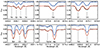 |
Fig. 8. Comparison of the observed (black lines) and theoretical spectra calculated with final parameters. Star 1 is represented by the blue line, and Star 2 by the red line. The spectra of Star 2 were shifted by subtracting a value of 0.1 from the flux. |
The effective temperatures of both components (Teff1 = 9800(100) K and Teff2 = 9200(200) K) and their surface gravities (( log g)1 = 4.1(1) and ( log g)2 = 4.0(1) cm s−2) suggest that both stars are of A0-A3 V spectral types. Both system components are slow-rotators with v sin i = 19(1) km s−1.
We estimated abundances for 29 elements (see Table 4). The number of lines used for the abundance estimation is given in columns denoted as ‘Nr’. The Fe abundance is the most robust measurement, based on 207 and 206 spectral lines for the primary and secondary components, respectively. The Fe abundances differ slightly between components ([Fe/H]prim = 0.21(9) and [Fe/H]sec = 0.08(10)) but are consistent within their errors. Both [Fe/H] values are in line with the catalogue value (Gaia Collaboration 2023) but are 0.3 dex higher than the SED-fitting results (Sect. 4). The abundances of iron-peak and rare-earth elements, combined with slow rotation, indicate chemical peculiarity in both components, as discussed in Sect. 6.3.
6. Discussion
6.1. Rotation
Slow to moderate rotation is critical for chemical peculiarity. In AmFm stars, the rotation rate should not exceed around 120 km s−1 (Abt & Moyd 1973; Michaud et al. 1983). The rotation velocity of the components, vrot, 1, 2 = v sin i/sin i ≈ 24.8 km s−1 (see Table 3), is well below this limit and is typical for AmFm stars (see the distribution of rotational velocities in Royer et al. 2007; Trust et al. 2020; Qin et al. 2021; Niemczura et al. 2017).
Using the values of R1, 2, (v sin i)1, 2, and i from Table 3 (and their uncertainties), we calculate the rotational frequencies of both components frot, 1, 2, and their errors. We determine the rotation period by solving the standard relation (e.g. Preston 1971)
 (5)
(5)
and use the propagation of errors law. We derive rotational frequencies of f1, rot = 0.238(17) and f2, rot = 0.246(17) c/d, consistent with the orbital frequency forb = 0.2428529(1) c/d. This suggests that the value of the inclination is well-established and that the system is relaxed with a circularised orbit and synchronous rotation of the components. The assumption of circular orbit and synchronously rotating components is further reinforced by the following angular momentum investigation.
The tidal equilibrium of the system is only possible if the total angular momentum, Ltot (a sum of the orbital and spin momenta), exceeds the critical momentum, Lcrit, calculated as per Ogilvie (2014):
 (6)
(6)
where M = M1 + M2 is the total mass of the stars (values from PHOEBE in Table 3), I = I1 + I2 is the total spin momentum of inertia of the stars, and μ = M1M2/(M1 + M2). The spin moment of inertia of the stars was calculated as  with M* and R* from Table 3 and β = 0.218 for stars with M = 2 M⊙ from Claret & Gimenez (1989).
The total angular momentum of the system, Ltot, is given by:
 (7)
(7)
and is dominated by the orbital angular momentum, Lorb, that can be expressed as
 (8)
(8)
where Ω = 2πforb rad s−1 is the angular velocity. If we assume that the spin angular velocity of the stars is equal to the orbital angular velocity (the calculated rotational frequencies match the orbital frequency), then Lorb ≈ 380Lspin. The total angular momentum, Ltot ∼ 2.5Lcrit, indicates that the system is in tidal equilibrium, while Lorb ≫ 3Lspin indicates that the system is relaxed with a stable tidal equilibrium resulting in a circular orbit and synchronous rotation of the components (Hut 1980; Ogilvie 2014). Carquillat & Prieur (2007) identified a circularisation cut-off period of 5.6(5) days (forb ≥ 0.179 c/d) for AmFm stars. All observational indices support the synchronous rotation of 50 Dra components with an orbital frequency of 0.243 c/d.
6.2. Additional variability
Since both components are almost equal, assigning the additional variability (manifesting as a group of peaks in the frequency spectra; Figs. 1 and 4) to either star is challenging. The unresolved frequency patterns suggest that it results from stochastic semi-regular or unresolved regular variability. In cold stars, such variations can be associated with magnetic activity, cold spots, their finite life span, and differential surface rotation. Although not expected in A-type stars (including AmFm stars), rotational variability analogous to cold stars likely connected with spots has been reported (e.g. Balona 2011; Sikora et al. 2019; Trust et al. 2020).
Stellar spots in cold stars are linked to local magnetic fields. Cantiello & Braithwaite (2019) demonstrated that spots in A-type stars can be induced by local magnetic fields generated by convection in thin sub-surface zones due to high opacity and/or low adiabatic gradient in the ionisation zones of H, He, and/or Fe. Weak magnetic fields have been detected in a few AmFm stars (e.g. Blazère et al. 2016a,b). In particular, the 50 Dra components resemble Sirius A, which is also an AmFm star, where a very weak magnetic field of 0.2 ± 0.1 G was detected (Petit et al. 2011), suggesting that this mechanism could operate in 50 Dra. However, the spot scenario is less likely because the group of peaks has a higher frequency than the rotational frequency (see Sect. 6.1) and is distinct from it (see Fig. 4). Such behaviour would require spots confined to higher latitudes (avoiding areas close to the equator) and polar regions rotating faster than equatorial regions. However, latitudinal differential rotation in the context of binarities remains poorly understood. The centre of the power hump is only about 10 % higher than the value of f2, rot, indicating that differential rotation may still be a plausible explanation that cannot be fully ruled out.
The group of frequencies (hump) may originate from unresolved prograde g-modes at frequencies higher than the rotational frequency. Similar features have been reported by Saio et al. (2018) and Henriksen et al. (2023a,b). For 50 Dra, the difference between the hump and the rotational frequency is only around 0.03 c/d, while the calculation for a star with two solar masses by Henriksen et al. (2023b) suggests a frequency separation of about 0.2 c/d. However, 50 Dra is about 2500 K hotter than their model star and its rotation rate is about four times lower. The g-mode explanation for the hump in 50 Dra requires detailed modelling, as g-mode excitation – as seen in γ Dor stars – is not expected and rarely observed at these temperatures (Guzik et al. 2000; Dupret et al. 2005; Dürfeldt-Pedros et al. 2024).
6.3. Chemical peculiarity
To assess the chemical peculiarity of 50 Dra components, we calculated average abundances of CP stars from the catalogue of Ghazaryan et al. (2018) and compared them with those of both components listed in Table 4. The abundances of particular elements in the stars AmFm (118 stars), HgMn (112 stars), and ApBp (188 stars) have typical uncertainties of 0.35, 0.65 and 0.60 dex, respectively. For stars with normal abundances, we used the sample of 33 stars from Niemczura et al. (2017) with a typical uncertainty of the abundance value of 0.39 dex. We also plotted the mean element abundances of 62 Am stars from Catanzaro et al. (2019, their table 3).
Comparison of catalogue values with abundances of 50 Dra components listed in Table 4, shows that both stars follow the sequence of AmFm stars (Fig. 9), with low abundance of Sc and overabundant heavy and rare-earth elements. We note that the mean values of the AmFm stars from Ghazaryan et al. (2018) differ from those of Catanzaro et al. (2019), increasing the range of possible values for the AmFm stars.
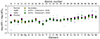 |
Fig. 9. Comparison of the mean element abundances of different classes of chemically peculiar stars (Ghazaryan et al. 2018; Catanzaro et al. 2019), normal stars (Niemczura et al. 2017) and 50 Dra components (magenta circles and yellow diamonds). The abundances of both stars of 50 Dra follow the AmFm abundances (green crosses and circles). |
Previous studies have shown that more than 70 % of AmFm stars reside in binary systems (e.g. Abt & Levy 1985; Carquillat & Prieur 2007). In addition, AmFm stars tend to appear in tight binaries with periods under 20 days (peaking near 5 days) (Carquillat & Prieur 2007). It is believed that the tidal forces in binary systems play a crucial role in slowing down the rotation of these stars, enabling atomic diffusion and the emergence of the chemical peculiarity observed in AmFm stars. In this context, 50 Dra is considered a typical representative of this category of CP stars.
Am stars predominantly exhibit temperatures between 7250 and 8250 K, peaking at 7750 K (Qin et al. 2019). From their collection of 9372 Am stars, Qin et al. (2019) found that only 32 stars have temperatures higher than 9000 K and only five were hotter than 9500 K. However, Catanzaro et al. (2019) identified that 15 of their 62 Am sample stars have temperatures above 9500 K, based on SED fitting. The components of 50 Dra thus represent a small group of hot Am stars.
7. Conclusions
We analysed 20 high-resolution spectra from the OES spectrograph (Koubský et al. 2004; Kabáth et al. 2020) together with photometric data from TESS (Ricker et al. 2015) to investigate 50 Dra. We modelled the radial velocity curve and photometric data, revealing that the system consists of two intermediate-mass stars with nearly equal masses close to 2 M⊙ (q = 0.951). The system exhibits an orbital period of 4.117719(2) days and an inclination of i = 49.9(8) deg, displaying ellipsoidal variations. Our investigation shows that both components are slow rotators (v sin i = 19(1) km s−1) in synchronous rotation with the orbital period.
Based on the analysis of separated spectra and comparison with catalogue values, it was determined that both stars in the system are metallic-line AmFm CP stars with temperatures of 9800 and 9200 K. The high temperatures indicate that the components of 50 Dra belong to a less common group of AmFm stars with temperatures above 9000 K. Beyond the effects of binarity, such as ellipsoidal variation, reflection effect, and beaming, the only feature detected in the frequency spectrum was the hump at 0.275 c/d. As the most probable explanation of this structure, we assume the presence of prograde g-modes. No signs of p-mode pulsations, which are rare in this temperature region (Dürfeldt-Pedros et al. 2024), or other signs of variability were found. We were unable to assign the hump feature to either component due to their near-identical properties.
It is worth noting that the short period may arise from binarity that has not been addressed in Trust et al. (2020).
HD 174257 (V = 7.53 mag) and HD 176795 (V = 6.71 mag).
Acknowledgments
We thank the referee for useful comments that helped to improved the manuscript. MS is grateful to T. van Reeth for the discussion about the nature of the additional variations and to P. Gajdoš for reading the manuscript. We would like to thank the observers for their work. MS acknowledges the support by Inter-transfer grant no LTT-20015. PK acknowledges the funding from ESA PRODEX PEA 4000127913. The calculations have been partly carried out using resources provided by the Wrocław Centre for Networking and Supercomputing (http://www.wcss.pl), Grant No 214. This paper includes data collected with the TESS mission and with the Perek telescope at the Astronomical Institute of the Czech Academy of Sciences in Ondřejov. Funding for the TESS mission is provided by the NASA Explorer Program. Funding for the TESS Asteroseismic Science Operations Centre is provided by the Danish National Research Foundation (Grant agreement no.: DNRF106), ESA PRODEX (PEA 4000119301) and Stellar Astrophysics Centre (SAC) at Aarhus University. We thank the TESS team and staff and TASC/TASOC for their support of the present work. We also thank the TASC WG4 team for their contribution to the selection of targets for 2-minute observations. The TESS data were obtained from the MAST data archive at the Space Telescope Science Institute (STScI). This research made use of NASA’s Astrophysics Data System Bibliographic Services, and of the SIMBAD database, operated at CDS, Strasbourg, France.
References
- Abt, H. A. 1961, ApJS, 6, 37 [NASA ADS] [CrossRef] [Google Scholar]
- Abt, H. A. 1981, ApJS, 45, 437 [NASA ADS] [CrossRef] [Google Scholar]
- Abt, H. A., & Levy, S. G. 1985, ApJS, 59, 229 [NASA ADS] [CrossRef] [Google Scholar]
- Abt, H. A., & Morrell, N. I. 1995, ApJS, 99, 135 [Google Scholar]
- Abt, H. A., & Moyd, K. I. 1973, ApJ, 182, 809 [NASA ADS] [CrossRef] [Google Scholar]
- Antoci, V., Cunha, M., Houdek, G., et al. 2014, ApJ, 796, 118 [Google Scholar]
- Antoci, V., Cantiello, M., Khalack, V., et al. 2025, A&A, 697, A111 [Google Scholar]
- Asplund, M., Grevesse, N., & Sauval, A. J. 2005, ASP Conf. Ser., 336, 25 [Google Scholar]
- Asplund, M., Grevesse, N., Sauval, A. J., & Scott, P. 2009, ARA&A, 47, 481 [NASA ADS] [CrossRef] [Google Scholar]
- Balona, L. A. 2011, MNRAS, 415, 1691 [NASA ADS] [CrossRef] [Google Scholar]
- Balona, L. A. 2013, MNRAS, 431, 2240 [NASA ADS] [CrossRef] [Google Scholar]
- Balona, L. A., Baran, A. S., Daszyńska-Daszkiewicz, J., & De Cat, P. 2015, MNRAS, 451, 1445 [Google Scholar]
- Blazère, A., Neiner, C., & Petit, P. 2016a, MNRAS, 459, L81 [CrossRef] [Google Scholar]
- Blazère, A., Petit, P., Lignières, F., et al. 2016b, A&A, 586, A97 [NASA ADS] [CrossRef] [EDP Sciences] [Google Scholar]
- Blazère, A., Petit, P., Neiner, C., et al. 2020, MNRAS, 492, 5794 [CrossRef] [Google Scholar]
- Bressan, A., Marigo, P., Girardi, L., et al. 2012, MNRAS, 427, 127 [NASA ADS] [CrossRef] [Google Scholar]
- Cantiello, M., & Braithwaite, J. 2019, ApJ, 883, 106 [Google Scholar]
- Carquillat, J. M., & Prieur, J. L. 2007, MNRAS, 380, 1064 [NASA ADS] [CrossRef] [Google Scholar]
- Catanzaro, G., Busà, I., Gangi, M., et al. 2019, MNRAS, 484, 2530 [NASA ADS] [CrossRef] [Google Scholar]
- Catanzaro, G., Frasca, A., Alonso-Santiago, J., & Colombo, C. 2024, A&A, 685, A133 [NASA ADS] [CrossRef] [EDP Sciences] [Google Scholar]
- Charbonneau, P., & Michaud, G. 1991, ApJ, 370, 693 [Google Scholar]
- Claret, A. 2003, A&A, 406, 623 [NASA ADS] [CrossRef] [EDP Sciences] [Google Scholar]
- Claret, A., & Gimenez, A. 1989, A&AS, 81, 37 [Google Scholar]
- Claret, A., Cukanovaite, E., Burdge, K., et al. 2020, A&A, 641, A157 [NASA ADS] [CrossRef] [EDP Sciences] [Google Scholar]
- Conroy, K. E., Kochoska, A., Hey, D., et al. 2020, ApJS, 250, 34 [Google Scholar]
- Cutri, R. M., Skrutskie, M. F., van Dyk, S., et al. 2003, VizieR On-line Data Catalog: II/246 [Google Scholar]
- Cutri, R. M., Wright, E. L., Conrow, T., et al. 2021, VizieR On-line Data Catalog: II/328 [Google Scholar]
- da Silva, L., Girardi, L., Pasquini, L., et al. 2006, A&A, 458, 609 [NASA ADS] [CrossRef] [EDP Sciences] [Google Scholar]
- Dupret, M. A., Grigahcène, A., Garrido, R., Gabriel, M., & Scuflaire, R. 2005, A&A, 435, 927 [NASA ADS] [CrossRef] [EDP Sciences] [Google Scholar]
- Dürfeldt-Pedros, O., Antoci, V., Smalley, B., et al. 2024, A&A, 690, A104 [NASA ADS] [CrossRef] [EDP Sciences] [Google Scholar]
- Eker, Z., Bakış, V., Bilir, S., et al. 2018, MNRAS, 479, 5491 [NASA ADS] [CrossRef] [Google Scholar]
- Gaia Collaboration (Brown, A. G. A., et al.) 2018, A&A, 616, A1 [NASA ADS] [CrossRef] [EDP Sciences] [Google Scholar]
- Gaia Collaboration (Brown, A. G. A., et al.) 2021, A&A, 649, A1 [NASA ADS] [CrossRef] [EDP Sciences] [Google Scholar]
- Gaia Collaboration (Vallenari, A., et al.) 2023, A&A, 674, A1 [NASA ADS] [CrossRef] [EDP Sciences] [Google Scholar]
- Ghazaryan, S., Alecian, G., & Hakobyan, A. A. 2018, MNRAS, 480, 2953 [NASA ADS] [CrossRef] [Google Scholar]
- Gontcharov, G. A. 2006, Astron. Lett., 32, 759 [Google Scholar]
- Gray, R. O., Corbally, C. J., De Cat, P., et al. 2016, AJ, 151, 13 [Google Scholar]
- Guzik, J. A., Kaye, A. B., Bradley, P. A., Cox, A. N., & Neuforge, C. 2000, ApJ, 542, L57 [Google Scholar]
- Hadrava, P. 1995, A&AS, 114, 393 [NASA ADS] [Google Scholar]
- Hadrava, P. 2004, Publ. Astron. Inst. Czechoslovak Acad. Sci., 92, 15 [Google Scholar]
- Harper, W. E. 1919, JRASC, 13, 236 [Google Scholar]
- Henriksen, A. I., Antoci, V., Saio, H., et al. 2023a, MNRAS, 520, 216 [NASA ADS] [CrossRef] [Google Scholar]
- Henriksen, A. I., Antoci, V., Saio, H., et al. 2023b, MNRAS, 524, 4196 [NASA ADS] [CrossRef] [Google Scholar]
- Høg, E., Fabricius, C., Makarov, V. V., et al. 2000, A&A, 355, L27 [Google Scholar]
- Huang, C. X., Vanderburg, A., Pál, A., et al. 2020a, Res. Notes Am. Astron. Soc., 4, 204 [Google Scholar]
- Huang, C. X., Vanderburg, A., Pál, A., et al. 2020b, Res. Notes Am. Astron. Soc., 4, 206 [Google Scholar]
- Husser, T.-O., Wende-von Berg, S., Dreizler, S., et al. 2013, A&A, 553, A6 [NASA ADS] [CrossRef] [EDP Sciences] [Google Scholar]
- Hut, P. 1980, A&A, 92, 167 [NASA ADS] [Google Scholar]
- Jenkins, J. M., Twicken, J. D., McCauliff, S., et al. 2016, SPIE Conf Ser, 9913, 99133E [Google Scholar]
- Kabáth, P., Skarka, M., Sabotta, S., et al. 2020, PASP, 132, 035002 [CrossRef] [Google Scholar]
- Kochukhov, O., Adelman, S. J., Gulliver, A. F., & Piskunov, N. 2007, Nat. Phys., 3, 526 [NASA ADS] [CrossRef] [Google Scholar]
- Kochukhov, O., Khalack, V., Kobzar, O., et al. 2021, MNRAS, 506, 5328 [NASA ADS] [CrossRef] [Google Scholar]
- Kochukhov, O., Gürsoytrak Mutlay, H., Amarsi, A. M., et al. 2023, MNRAS, 521, 3480 [NASA ADS] [CrossRef] [Google Scholar]
- Koubský, P., Mayer, P., Čáp, J., et al. 2004, Publ. Astron. Inst. Czechoslovak Academy Sci., 92, 37 [Google Scholar]
- Kurtz, D. W. 1989, MNRAS, 238, 1077 [NASA ADS] [Google Scholar]
- Kurucz, R. L. 2005, Mem. Soc. Astron. It. Suppl., 8, 14 [Google Scholar]
- Lightkurve Collaboration (Cardoso, J. V. d. M., et al.) 2018, Astrophysics Source Code Library [record ascl: 1812.013] [Google Scholar]
- Barentsen, G., & Lightkurve Collaboration 2020, Am. Astron. Soc. Meeting Abstr., 235, 409.04 [Google Scholar]
- Michaud, G. 1970, ApJ, 160, 641 [Google Scholar]
- Michaud, G., Tarasick, D., Charland, Y., & Pelletier, C. 1983, ApJ, 269, 239 [Google Scholar]
- Murphy, S. J., Saio, H., Takada-Hidai, M., et al. 2020, MNRAS, 498, 4272 [NASA ADS] [CrossRef] [Google Scholar]
- Nguyen, C. T., Costa, G., Girardi, L., et al. 2022, A&A, 665, A126 [NASA ADS] [CrossRef] [EDP Sciences] [Google Scholar]
- Niemczura, E., Murphy, S. J., Smalley, B., et al. 2015, MNRAS, 450, 2764 [Google Scholar]
- Niemczura, E., Polińska, M., Murphy, S. J., et al. 2017, MNRAS, 470, 2870 [Google Scholar]
- Ogilvie, G. I. 2014, ARA&A, 52, 171 [Google Scholar]
- Paegert, M., Stassun, K. G., Collins, K. A., et al. 2021, ArXiv e-prints [arXiv:2108.04778] [Google Scholar]
- Paunzen, E. 2015, A&A, 580, A23 [NASA ADS] [CrossRef] [EDP Sciences] [Google Scholar]
- Petit, P., Lignières, F., Aurière, M., et al. 2011, A&A, 532, L13 [NASA ADS] [CrossRef] [EDP Sciences] [Google Scholar]
- Preston, G. W. 1971, PASP, 83, 571 [NASA ADS] [CrossRef] [Google Scholar]
- Preston, G. W. 1974, ARA&A, 12, 257 [Google Scholar]
- Pych, W. 2004, PASP, 116, 148 [NASA ADS] [CrossRef] [Google Scholar]
- Qin, L., Luo, A. L., Hou, W., et al. 2019, ApJS, 242, 13 [NASA ADS] [CrossRef] [Google Scholar]
- Qin, L., Luo, A. L., Hou, W., et al. 2021, AJ, 162, 32 [Google Scholar]
- Ricker, G. R., Winn, J. N., Vanderspek, R., et al. 2015, J. Astron. Telescopes Instrum. Syst., 1, 014003 [Google Scholar]
- Rodrigues, T. S., Girardi, L., Miglio, A., et al. 2014, MNRAS, 445, 2758 [Google Scholar]
- Rodrigues, T. S., Bossini, D., Miglio, A., et al. 2017, MNRAS, 467, 1433 [NASA ADS] [Google Scholar]
- Royer, F., Zorec, J., & Gómez, A. E. 2007, A&A, 463, 671 [NASA ADS] [CrossRef] [EDP Sciences] [Google Scholar]
- Saio, H., Kurtz, D. W., Murphy, S. J., Antoci, V. L., & Lee, U. 2018, MNRAS, 474, 2774 [Google Scholar]
- Sbordone, L. 2005, Mem. Soc. Astron. It. Suppl., 8, 61 [Google Scholar]
- Sikora, J., David-Uraz, A., Chowdhury, S., et al. 2019, MNRAS, 487, 4695 [Google Scholar]
- Skarka, M., Žák, J., Fedurco, M., et al. 2022, A&A, 666, A142 [NASA ADS] [CrossRef] [EDP Sciences] [Google Scholar]
- Smalley, B., Antoci, V., Holdsworth, D. L., et al. 2017, MNRAS, 465, 2662 [NASA ADS] [CrossRef] [Google Scholar]
- Tody, D. 1986, SPIE Conf. Ser., 627, 733 [Google Scholar]
- Trust, O., Jurua, E., De Cat, P., & Joshi, S. 2020, MNRAS, 492, 3143 [NASA ADS] [CrossRef] [Google Scholar]
- Twicken, J. D., Chandrasekaran, H., Jenkins, J. M., et al. 2010, SPIE Conf. Ser., 7740, 77401U [Google Scholar]
- Vines, J. I., & Jenkins, J. S. 2022, MNRAS, 513, 2719 [NASA ADS] [CrossRef] [Google Scholar]
- Wilson, R. E. 1953, General catalogue of stellar radial velocities (Washington D.C.: Carnegie Institute Washington Publication) [Google Scholar]
- Zucker, S., Mazeh, T., & Alexander, T. 2007, ApJ, 670, 1326 [NASA ADS] [CrossRef] [Google Scholar]
Appendix A: Supporting material
Stars in the vicinity of 50 Dra shown in Fig. 2.
Magnitudes used for SED fitting.
Radial velocities of both components in km s−1.
All Tables
All Figures
|
Fig. 1. Comparison of the available data products generated by different pipelines (top panel) and corresponding frequency spectra with labelled features (bottom panel). |
| In the text | |
|
Fig. 2. Vicinity of 50 Dra showing the aperture mask in Sector 14 with identification of possible contaminants identified in Table A.1. The field size shown in the figure is approximately 4 × 4 arcmin. |
| In the text | |
|
Fig. 3. TESS SC data of 50 Dra phase-folded with the orbital period. Each circle corresponds to the mean of 4400 individual TESS observations. |
| In the text | |
|
Fig. 4. Frequency spectrum centred around a group of peaks produced by additional variability from different data segments (coloured lines) and the full data set (black line). The amplitude of the frequency spectrum of the full dataset is multiplied by two for better readability. The black dashed line denotes the position of the orbital and rotational frequency. |
| In the text | |
|
Fig. 5. Spectral energy distribution (SED) derived from photometric observations (Table A.2) using ARIADNE. |
| In the text | |
|
Fig. 6. Top: Observed spectra in different orbital phases around the Mg I 5167–5183 Å triplet and Fe II 5169 Å lines. The mean disentangled spectra for the primary and secondary components are shown in blue and red, respectively. Bottom: Trails of Na D, Si II, and Hα lines (from left to right) showing the variation of the position of the lines of both components during the orbital cycle. The relative intensity of the lines is also indicated. |
| In the text | |
|
Fig. 7. Radial velocity curve of both components with the best fit (upper panel) and the light curve with the best fit (bottom panel). The photometric points are binned to produce 500 points per orbital phase. |
| In the text | |
|
Fig. 8. Comparison of the observed (black lines) and theoretical spectra calculated with final parameters. Star 1 is represented by the blue line, and Star 2 by the red line. The spectra of Star 2 were shifted by subtracting a value of 0.1 from the flux. |
| In the text | |
|
Fig. 9. Comparison of the mean element abundances of different classes of chemically peculiar stars (Ghazaryan et al. 2018; Catanzaro et al. 2019), normal stars (Niemczura et al. 2017) and 50 Dra components (magenta circles and yellow diamonds). The abundances of both stars of 50 Dra follow the AmFm abundances (green crosses and circles). |
| In the text | |
Current usage metrics show cumulative count of Article Views (full-text article views including HTML views, PDF and ePub downloads, according to the available data) and Abstracts Views on Vision4Press platform.
Data correspond to usage on the plateform after 2015. The current usage metrics is available 48-96 hours after online publication and is updated daily on week days.
Initial download of the metrics may take a while.