| Issue |
A&A
Volume 698, June 2025
|
|
|---|---|---|
| Article Number | A63 | |
| Number of page(s) | 9 | |
| Section | Extragalactic astronomy | |
| DOI | https://doi.org/10.1051/0004-6361/202452323 | |
| Published online | 28 May 2025 | |
The Pristine Dwarf-Galaxy survey
VI. A VLT/FLAMES spectroscopic study of the dwarf galaxy Boötes II
1
Laboratoire d’astrophysique, École Polytechnique Fédérale de Lausanne (EPFL), Observatoire, 1290 Versoix, Switzerland
2
IFCA, Instituto de Física de Cantabria (UC-CSIC), Av. de Los Castros s/n, 39005 Santander, Spain
3
GEPI, Observatoire de Paris, Université PSL, CNRS, Place Jules Janssen, F-92195 Meudon, France
4
Instituto de Astrofísica de Canarias, Calle Vía Láctea s/n, 38206 La Laguna, Santa Cruz de Tenerife, Spain
5
Universidad de La Laguna, Avda. Astrofísico Francisco Sánchez, 38205 La Laguna, Santa Cruz de Tenerife, Spain
6
Max-Planck-Institut für Astronomie, Königstuhl 17, D-69117 Heidelberg, Germany
7
Myrspoven AB, Västgötagatan 1, 11827 Stockholm, Sweden
8
Université de Strasbourg, CNRS, Observatoire astronomique de Strasbourg, UMR 7550, F-67000 Strasbourg, France
9
Dept. of Physics and Astronomy, University of Victoria, PO Box 3055, STN CSC Victoria, BC V8W 3P6, Canada
10
Centre for Astrophysics Research, Department of Physics, Astronomy and Mathematics, University of Hertfordshire, Hatfield AL10 9AB, UK
⋆ Corresponding author.
Received:
20
September
2024
Accepted:
4
April
2025
Abstract
Aims. The Milky Way has a large population of dwarf galaxy satellites. Their properties are sensitive to both cosmology and the physical processes underlying galaxy formation, but these properties are still not properly characterised for the entire satellite population.
Methods. We aim to provide the most accurate systemic dynamical and metallicity properties of the dwarf galaxy Boötes II (Boo II).
Results. We use a new spectroscopic sample of 39 stars in the field of Boo II (heliocentric distance of ∼66 kpc) with data from the Fiber Large Array Multi Element Spectrograph (FLAMES) mounted on the Very Large Telescope (VLT). The target selection is based on a combination of broadband photometry, proper motions from Gaia, and the metallicity-sensitive narrow-band photometry from the Pristine survey that is ideal for removing obvious Milky Way contaminants.
Conclusions. We found nine new members, including five also found by recent works in the literature, and the farthest member to date (5.7 half-light radii from Boo II centroid), extending the spectroscopic spatial coverage of this system. Our metallicity measurements based on the Calcium triplet lines leads to the detection of the two first Extremely Metal-poor stars ([Fe/H] < −3.0) in Boo II. Combining this new dataset with literature data refines Boo II’s velocity dispersion (5.6−1.1+1.8 km s−1), systemic velocity (−126.8−1.5+2.0 km s−1), and shows that it does not show any sign of a significant velocity gradient (d⟨v⟩/dχ = 0.6−0.4+0.6 km s−1 arcmin−1, or −0.5/1.9 km s−1 arcmin−1 as 3σ upper limits). We are thus able to confirm the kinematic and metallicity properties of the satellite as well as identify new members for future high-resolution analyses.
Key words: galaxies: individual: Boötes II / Local Group
© The Authors 2025
 Open Access article, published by EDP Sciences, under the terms of the Creative Commons Attribution License (https://creativecommons.org/licenses/by/4.0), which permits unrestricted use, distribution, and reproduction in any medium, provided the original work is properly cited.
This article is published in open access under the Subscribe to Open model. This email address is being protected from spambots. You need JavaScript enabled to view it. to support open access publication.
1. Introduction
The successive large-coverage photometric surveys over the last two decades, from the Sloan Digital Sky Survey (York et al. 2000, SDSS), the Panoramic Survey Telescope And Rapid Response System (Chambers et al. 2016, PS1), or the Dark Energy Survey (The Dark Energy Survey Collaboration 2005, DES), to the upcoming Legacy Survey of Space and Time (Ivezić et al. 2019, LSST), have led to the discovery of dozens of faint galaxy companions orbiting the Milky Way (MW). The faintest ones are usually referred to as ultra-faint dwarf galaxies (UFD).
The current UFD population of the MW has been extensively studied. Their morphological properties (morphology, luminosity, mass) as well as their spectroscopic properties (metallicity, chemical enrichment, orbit) were an immediate focus point of the community. Most UFD studies have a singular goal: to compare their observed morphology with the ones predicted by the various numerical simulations made throughout the years (e.g. Sawala et al. 2016 or Read & Erkal 2019 for the mass, Revaz 2023 for the morphology, Sanati et al. 2023 for the stellar abundances, Sanati et al. 2024 for the mass and stellar population). In doing so, we are able to improve our understanding not only of the cosmological significance of UFDs (e.g. Springel et al. 2008; Read & Erkal 2019; Revaz 2023) but also of the physical processes linked to the formation and evolution of galaxies, such as stellar feedback (e.g. Agertz et al. 2020; Sanati et al. 2023).
Therefore, a large number of spectroscopic studies of UFDs has been carried out over the years. Until recently, the vast majority of these studies from different teams with different observational strategies using different observing facilities have had but one main goal: derive the intrinsic properties of the satellite (morphology, dynamical mass, stellar abundances). To do so, it is imperative to derive the membership of as many UFD stars as possible. A task made challenging by the foreground contamination of the MW stars.
The UFDs are usually approximated as ‘simple’ systems characterized by the mean and dispersion of their velocity and metallicity distributions, which are usually considered enough to offer a comprehensive view of their properties (Simon 2019 and references therein). This simplistic view of the UFDs’ stellar population is now more and more disputed with the rise of observing strategies specifically designed to more efficiently weed out the MW stellar contamination. This also allows to find more members with larger spatial coverage than before. These strategies essentially rest on the use of specific photometric bands that are able to trace the metal content of stars and to discard the obvious metal-rich population that should not inhabit UFDs (e.g. Longeard et al. 2021, 2022 for the Pristine survey, Chiti et al. 2021 for SkyMapper, or Pan et al. 2024 with DECam photometry). These studies indeed point towards a more complex picture for both their dynamical (i.e. the mass of all components of the galaxy, see Wolf et al. 2010 and Errani et al. 2018) and metallicity properties. In that sense, such spectroscopic studies are needed to paint the most accurate picture of the overall UFD population which is critical to properly constrain our cosmological and galaxy models by comparing observations with simulations.
The following work is directly related to this effort: we spectroscopically observed the UFD Boo II to enlarge the catalogue of member stars and to spatially extend this catalogue. Boo II has already been the subject of two past spectroscopic studies, Koch et al. (2009, K09) and Bruce et al. (2023, B23), with the latter published during the completion of this manuscript, after our observations had already been carried out and analysed. K09 used Gemini/GMOS multi-object spectroscopy (Hook et al. 2004) to find the first five members in the system and derived a systemic velocity of 117 ± 5.2 km s−1 and a large but highly uncertain velocity dispersion of 10.5 ± 7.4 km s−1. Their metallicity was found to be of −1.79 ± 0.05. Recently, B23 found nine new member stars and confirmed the membership of 3 stars of K09 using Magellan/IMACS spectroscopy (Dressler et al. 2011). In particular, B23 showed that the mean quantitative results of K09 were heavily biased with an updated velocity of  km s−1 and a metallicity of
  , most likely due to the observational setup used by K09 that is not ideal to derive accurate velocities although it is enough for membership inference. B23 also tightly constrained the velocity dispersion (
 km s−1) and therefore the mass-to-light ratio of Boo II (
 M⊙ L⊙−1). Their main results are summarized in Table 1.
Summary of Boo II’ prior literature (K09 and B23) properties. The reference numbers correspond to the following list: (1) Muñoz et al. (2018), (2) Walsh et al. (2008), (3) Koch et al. (2009), (4) Bruce et al. (2023), (5) Ji et al. (2016).
The following introduces our brand-new Boo II observations and subsequent dynamical and metallicity analyses. Section 2 details the data selection, observations and reduction procedures. Section 3 presents our membership, dynamical and metallicity results. Finally, Section 4 summarizes our findings and discusses our current knowledge of Boo II in the light of all the studies existing on this UFD.
2. Spectroscopic observations
This section provides details on the target selection, observations and data reduction first, then briefly explains our velocity and equivalent width (EW) derivation method.
2.1. Data selection
All targets were selected based on the colour–magnitude diagram (CMD), narrow-band photometry, and with Gaia astrometry, as detailed in the following subsections.
2.1.1. The Pristine survey selection
Pristine is a photometric survey (Starkenburg et al. 2017; Martin et al. 2024) relying on a narrow-band, metallicity-sensitive photometry centred on the Calcium H&K doublet lines from the Canadian France Hawaii Telescope (Boulade et al. 2003, CFHT). It is successful at finding metal-poor stars against the more metal-rich MW contamination (Youakim et al. 2017; Aguado et al. 2019; Arentsen et al. 2020) and is therefore particularly suited for the UFDs metal-poor population (Longeard et al. 2020, 2021, 2022). To derive the Pristine photometric metallicities, the procedure of Starkenburg et al. (2017) is followed and we refer the reader to their Section 3 for details. The main difference with Starkenburg et al. (2017) is that the Pristine survey footprint has since been greatly expanded. Therefore, our training sample to create the CaHK to [Fe/H] model is larger than theirs.
To summarize the process, Pristine observes stars with a narrow-band filter centred on the CaHK doublet lines. These stars also have a counterpart in SDSS to obtain classical, broadband photometry. To build the CaHK to [Fe/H] model, we restrict ourselves to stars observed with Pristine that also have an SDSS spectroscopic metallicity measurement. This training sample is cleaned from potential white dwarfs, mediocre CaHK and broadband photometry following the criteria of Starkenburg et al. (2017). The remaining stars are then placed in a g − i, CaHK − g − 1.5 × (g − i) colour-colour diagram. In this colour–colour space, they naturally separate as a function of their metallicity (Figure 11 of Starkenburg et al. 2017). By binning this colour–colour space and using the stars’ SDSS metallicities as a reference, we are able to calibrate this space and derive the photometric metallicity of any star with SDSS broadband and Pristine photometries.
2.1.2. Selection criteria
Three main criteria were applied to select potential members for our spectroscopic observations:
-
Stars located further than 0.2 mag from the best-matching Boo II isochrone (Age = 13 Gyr, [Fe/H] = −2.4, [α/Fe] = 0.0, m − M = 18.10) from the Darmouth library (Dotter et al. 2008) were discarded. The distance modulus was taken from Muñoz et al. (2018).
-
Their location on the Pristine colour–colour diagram must be located above the region occupied by the population of UFDs (Longeard et al. 2023), indicating a metallicity lower than that of the vast majority of MW stars. This roughly corresponds to metallicities lower than −1.0 dex.
-
The proper motion membership probability of all targets must be at least 1%, based on the Gaia Data Release 3 (Gaia Collaboration 2023). These membership probabilities are computed assuming two multivariate gaussian populations in proper motion space, for Boo II and the MW, respectively, based on the systemic proper motion of Battaglia et al. (2022) and McConnachie & Venn (2020).
2.2. Data acquisition
The spectroscopic sample was obtained using the Very Large Telescope (Pasquini et al. 2002, VLT) and its FLAMES multi-object spectrograph. The HR21 grating was used to encompass the calcium triplet (CaT) lines, with a spectral resolution R of ∼18 000. The observations were carried out throughout two semesters, from April 2022 to February 2023, observing nine sub-exposures of 2775 seconds each. Only the ninth sub-exposure were observed in February 2023, the rest being observed in April-May 2022. Unfortunately, this prevents us from performing a robust binary test between the sub-exposures carried out in 2022 and the one in 2023, since it requires to analyze the ninth exposure alone, which considerably reduces the SNR of each spectrum. However, this was performed when possible and the velocities between the 2022 and 2023 observations were consistent within their respective uncertainties, indicating that no obvious binaries might affect the results.
All sub-exposures are indicated as good-quality observations, that is graded A (8) or B (1) by the ESO observing team. To summarize, when requesting an observation at ESO, observational constraints are also provided. A grade A corresponds to the situation where all constraints are met, while B is for observations for which they were not all met, but were within 10% of the requested values. The field is centred on the system based on the coordinates of Muñoz et al. (2018). This field is shown in Figure 1 and extends as far as ∼8 half-light radii (rh) of Boötes II (Boo II).
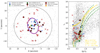 |
Fig. 1. Left panel: Spatial distribution of the FLAMES spectroscopic sample. Newly discovered members are shown as red diamonds. Non-members from the FLAMES sample are shown as red crosses. Previously known members from the literature (K09 + B23) are represented as smaller blue circles. Misidentified literature members are shown as green crosses. The two half-light radii of Boo II as inferred by Muñoz et al. (2018, M18) are shown as a black ellipse. The small grey dots show all stars in the field with good quality SDSS photometry (i.e. broadband photometry uncertainties below 0.2 mag). Right panel: CMD of our spectroscopic sample superimposed with the favoured Boo II Dartmouth isochrone in yellow, chosen to match the system’s spectroscopically identified RGB stars. Three other isochrones of varying metallicity (one more metal-poor at [Fe/H] ∼ −2.5, two more metal-rich at ∼ − 1.5 and ∼ − 1.2) are also overplotted as dashed green lines. The g and i magnitudes are from SDSS. |
The few unassigned fibers left were filled with even lower-priority stars and interesting, potentially extremely metal-poor (EMP, [Fe/H] < −3.0) MW halo stars in the field according to Pristine.
2.3. Data reduction
The standard ESO package to reduce GIRAFFE data (Melo et al. 2009) was used to reduce the data, without any modification to the pipeline.
Three examples of spectra for low (6.0), mid (15.0) and high (164) signal-to-noise ratios (S/Ns) per pixel are shown in Figure 2. Each spectrum was carefully visually inspected and discarded if its quality was too poor to obtain a proper fit of any of the three CaT lines. This mostly involves low S/N spectra below 3, but also mid S/N ones for which the CaT lines were too contaminated (from e.g. sky substraction) to be properly fitted. This step led to the rejection of five spectra.
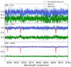 |
Fig. 2. Example spectra of three candidate member stars in our FLAMES dataset centred on the CaT lines. The low, mid and high S/N regimes are represented here. The normalised spectra are shown with solid blue lines while the fits derived from our pipeline for Voigt profiles are shown with solid red lines. Residuals in the Voigt cases are shown for each case below the spectra as dashed green lines. These stars have a heliocentric velocity of −133.2 ± 1.5 (the ‘metal-rich’ candidate in Figure 2), −111.3 ± 0.6 and −133.3 ± 0.2 km s−1 from top to bottom. |
We normalized the spectra following the method of Battaglia et al. (2008), that is through an iterative k-sigma clipping non-linear filter. The heliocentric velocities and equivalent widths (EWs) of each spectrum were then obtained using our in-house pipeline described in detail in Longeard et al. (2022), which has already been extensively tested against known metallicities and velocities and recently used by Longeard et al. (2023). Each CaT line was modelled with a Gaussian and Voigt profiles and their position was found by minimizing the squared difference between a synthetic spectrum composed of three Gaussian or Voigt profiles and the observed spectrum. The EWs were calculated by integrating the best fit around each line in a 15 Å window. This was performed with a Monte Carlo Markov chain (Hastings 1970) algorithm with a million iterations per spectrum. The MCMC produced posterior probability functions that allowed us to derive the uncertainty on each parameter.
The median of the velocity uncertainty is 1.2 km s−1 for the new FLAMES sample, 1.7 km s−1 for entire sample (literature + FLAMES, details in section 3.2) and 1.3 km s−1 when the sample is restricted to Boo II literature member stars only. Note that for the rest of this work, the ’literature’ refers to the two previous spectroscopic analysis of Boo II, that is B23 and K09. Figure 3 shows that our velocities agree very well with those of B23 for five member stars in common, and that FLAMES data reduce the velocity uncertainties by a factor of ∼2 on average.
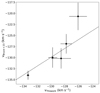 |
Fig. 3. Comparison between the heliocentric velocity of B23 and the ones found in this work for the members stars in common. |
The UFDs Leo IV and Leo V were also observed during this programme and subjected to the same data treatment. However, the lack of enough new members in our data explains that we do not analyse those data in more details in the following work.
3. Results
We present in this section the results of our analysis. The metallicity results will be presented first since they are needed to derive Boo II’s kinematic properties.
3.1. Metallicity properties
The metallicities of the stars in our sample are derived in two ways that will be presented below: 1) using spectra when the S/N is greater than 10 for the FLAMES and literature members, and 2) using the Pristine narrow-band, metallicity-sensitive data. For the latter, a calibration of the CaHK space for giant stars is used.
To derive the spectroscopic metallicities, we use the same process as in Longeard et al. (2022) and Longeard et al. (2023), that is derive the EWs of the three CaT lines, then use the calibration of Carrera et al. (2013) that translates them into a metallicity value with an associated uncertainty that takes into account the following sources: uncertainty on the EWs, the distance modulus, the photometry and the calibration’s coefficients. The results are reported in Table A.1 and shown in Figure 4. The left panel shows that we identify two members as EMPs, including one at the edge of the calibration range of Carrera et al. (2013) at ∼ − 4.0. The right panel shows that a bias exists between CaHK and spectroscopic metallicities of the order of ∼0.5 dex. We do not understand the source of this discrepancy, though it most likely stems from different photometric zero-points between all CCDs in the field. However, this does not impact our results since our Pristine-based selection does not rely on the metallicity value itself but on their location of the Pristine colour–colour diagram shown in Figure 5, and that our selection is quite generous on that colour space.
 |
Fig. 4. Metallicity distribution functions (MDFs) for the CaT (left) and CaHK (centre) cases. The right panel shows the comparison between the two metallicities, with the 1:1 line as the dashed black line. |
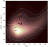 |
Fig. 5. CaHK colour–colour diagram, with the temperature proxy (g − i)0 on the x axis and the Pristine colour containing the metallicity-sensitive information. The density map in the background of the plot is produced using MW stars in the field of Boo II, with 1, 2 and 3σ contours shown as dotted white lines. In this diagram, the metallicity goes down as the y axis colour decreases. The dashed straight line shows the cut applied to the data to distinguish likely the metal-poor from the likely metal-rich stars. The colours and markers used are the same as those of Fig. 1. |
In the rest of this study, and coming from experience, stars with a CaHK uncertainty above 0.2 mag often yields mediocre or very uncertain photometric metallicities and their metallicities are not computed. The results are shown in the right panel of Figure 4. The right panel clearly shows a metallicity peak at around −2.0 that corresponds to Boo II’s population.
3.2. Analysis
To derive the dynamical properties of the system, we add more criteria to clean the sample besides the ones detailed in Section 2.1.2. These criteria are:
-
Their ratio of parallax over parallax uncertainty taken from Gaia must be lower than 2.0.
-
They must not have been identified as potentially variable-velocity stars in the literature.
Once all these criteria are applied, the final sample consists of 39 stars. Given the number of fibers that were still available after the cleaning of Section 2.1.2, we decided to observe probable MW halo stars flagged as metal-poor by the CaHK photometry as target of opportunities, even though they are not linked to the analysis and therefore not included in the 39 stars in the final sample.
The dynamical properties of Boo II are derived following the formalism of Martin & Jin (2010) combined with the likelihoods described in their Equations (2) and (3):
![Mathematical equation: $$ \begin{aligned}&\mathcal{L} (\mathrm{v}_{\mathrm{r},k}, \delta _{\mathrm{v},k} | \langle \mathrm{v}_{\mathrm{Boo}} \rangle , \langle \mathrm{v}_{\mathrm{MW}} \rangle , \sigma ^\mathrm{Boo}_{\mathrm{v}}, \sigma ^\mathrm{MW}_{\mathrm{v}}, \mathrm{d}\mathrm{v}/\mathrm{d}\chi , \theta , \eta _{\rm Boo}) \nonumber \\&=\prod _k \; \bigg [ \eta _{\rm Boo} (\frac{1}{\sqrt{2 \pi \sigma }}) \times \mathrm{exp}(\frac{1}{2}\Delta _{\rm v}/\sigma ^{2}) \mathcal{L} ^{\mathrm{Boo}}_{\mathrm{PM}}\\&+(1 - \eta _{\rm Boo}) \mathcal{G} (\mathrm{v}_{\mathrm{r},k}, \delta _{\mathrm{v},k},\langle \mathrm{v}_{\mathrm{MW}} \rangle , \sigma ^\mathrm{MW}_{\mathrm{v}}) \mathcal{L} ^{\mathrm{MW}}_{\mathrm{PM}} \bigg ].\nonumber \end{aligned} $$](/articles/aa/full_html/2025/06/aa52323-24/aa52323-24-eq13.gif) (1)
(1)
We define Δv such that Δv = vr, k − y × dv/dχ + ⟨vBooII⟩ with dv/dχ the systemic heliocentric velocity gradient, and χ the galacto-centric distance along the position angle θ. y is the angular distance computed such that yk = Xksinθ + Ykcosθ and θ the direction of the velocity gradient. We also define  , with
  the intrinsic Boo II velocity dispersion and δvk the individual velocity uncertainty of each star. Finally, ηBooII is the Boo II member fraction of the spectroscopic sample.
The final posterior probability distribution functions (PDFs) of Boo II’s dynamical properties are shown in Figure 6. This figure illustrates that our results are compatible with the ones of B23. To check the validity of our code, we first derived the systemic velocity and velocity dispersion of Boo II only using the dataset of B23 and found the dashed blue PDF. This PDF falls perfectly onto the green shaded area corresponding to the results reported by B23. This plot shows that Boo II does not show clear evidence of a velocity gradient.
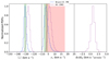 |
Fig. 6. Posterior PDFs of the main dynamical properties of Boo II, i.e. the systemic velocity (left panel), the intrinsic velocity dispersion (middle panel), and velocity gradient (right panel). The dashed blue PDFs show the results of our analysis using only the B23 sample. The purple PDF shows the result of this work using the entire sample (i.e. K09 + B23 + FLAMES). The shaded area indicates the 1σ interval inference of K09 (green) and B23 (red). This K09 interval is not shown for the systemic velocity as their velocity was strongly biased (∼ − 110 km s−1, and therefore outside the plot). |
From this analysis, we can derive the membership probability of all stars in the sample. To classify a star as a member, we add a 10% dynamical membership probability, computed from Equation (1), to the criteria detailed in Section 2.1.2 and the beginning of Section 3.2.
Nine new members are found in the new FLAMES dataset, including six also identified by B23. Furthermore, the membership status of one other star is debatable as it is located right in the MW region of the Pristine colour–colour diagram, with no proper motion information to help in the decision-making process (Figure 7) Its CMD location, bluer than the mean Boo II population in Figure 1, suggests a lower metallicity than that of the UFD. Furthermore, one star classified as a non-member in the literature is found to be a tentative member in this study. It is shown as a green circle in Figures 1, 5 and 7. Its velocity and photometric metallicity are perfectly compatible with Boo II. However, it does not have a PM measurement, and its CMD location is ∼0.15 mag redder than that of the mean Boo II population, which prevents us from being certain of its membership. Three likely misidentified members from the literature, shown as green crosses, are also identified. Their properties are shown in Table A.3. Finally, the different membership probability components are detailed in Table A.2.
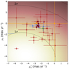 |
Fig. 7. Proper motions of the full spectroscopic sample. The plot is restricted to an area around the proper motion of Boo II for the sake of visibility, but other stars (clearly non-members) are located outside this region. The density background shows the density of MW star in the field of Boo II, with 1 and 2σ contours shown as dashed black lines. The colour and marker schemes are the same as in previous plots. |
The entire dataset’s velocity, metallicity and position along Boo II’s major-axis are summarized in Figure 8. This plot is also useful to investigate any significant velocity and/or metallicity gradient along Boo II major axis. The visual impression confirms our quantitative analysis below in that there does not seem to be any radial trend on any of the two properties. The lower panel of this plot also illustrates once more that the Pristine metallicities are overestimated when compared to their spectroscopic counterparts, when available.
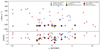 |
Fig. 8. Summary of the velocity and metallicity measurements of the spectroscopic sample to investigate potential velocity and/or metallicity gradients. The velocity uncertainties are reported in the plot but are so small compared to the scale of the y axis that they are overall not visible, except for a few cases with extremely large uncertainties. Top panel: velocity vs. position along Boo II’s major axis. The colour and marker schemes are similar to what was shown in the previous plots. The literature (i.e. K09 + B23) and new members do not display any sign of a velocity gradient, even by including the potential more metal-rich member candidate at χ ∼ −10 arcmin. Lower panel: CaT (with black contours) and CaHK (without contours) metallicities. In the case where both are available for the same star, the two values are linked by a dashed grey line. |
The recent work of Pan et al. (2024) derives photometric metallicities and therefore promising candidates for Boo II from their DECam photometry. Their table of candidates contains two (RA = 209.49804167deg, Dec = 12.86472222deg – RA = 209.5725deg, Dec = 12.8035deg) of our new members (not the ones in common with B23). Each of them is classified as a ’candidate with low purity due to its faintness’ by Pan et al. (2024).
Finally, we find a systemic velocity ( km s−1) and velocity dispersion
  km s−1) slightly larger, but statistically compatible with B23 at the 1σ level. The existence of a velocity gradient is investigated for the first time, and this investigation shows that Boo II shows no convincing sign of a significant velocity gradient: it is consistent with the null hypothesis at the 1.5σ level (
 km s−1). This implies that the Boo II mass is not biased by tidal interactions or any unexpected internal velocity distribution.
4. Summary and conclusion
We present new spectroscopic observations with the FLAMES/VLT spectrograph, of candidate member stars in and around the faint UFD Boo II. Our initial selection was based on the combination of the Pristine narrow-band photometry, broad band optical colours, and Gaia DR3 proper motions. We analyse the CaT region of 39 spectra with SNR ≥ 3, of stars distributed over a region reaching ∼8 rh from the galaxy centre. We combine our new sample with previously published datasets, and can derive the most robust dynamical and metallicity properties of Boo II to date. In particular, we report the discovery of 9 new member stars, including 6 in common with B23. One additional star, apparently metal-rich, is located at ∼4 rh of the satellite. While it has the right velocity, its CaHK photometry places it on the MW locus and it has no proper motion measurement. Future spectroscopic programmes should confirm its membership.
All the confirmed members now have improved velocity measurements thanks to our FLAMES programme and, more specifically, the use of the HR21 grating and with higher resolution than the spectroscopic setups previously used. We derive the metallicity of 8 stars and double the number of stars with chemical information. We confirm the very metal-poor nature of the system. Moreover, we provide the identification of two spectroscopically EMP stars in Boo II.
We find a systemic velocity of 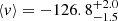 km s−1 and a dispersion of
  km s−1. We note the possibility of a slight velocity gradient, but it is nevertheless still compatible with no velocity gradient at the ∼1.5σ level.
We also obtained spectroscopic data for two other UFDs, Leo IV and Leo V, but were only able to identify one new member which does not change our view of the two systems.
Acknowledgments
This work has been carried out thanks to the support of the Swiss National Science Foundation. Based on observations obtained with MegaPrime/MegaCam, a joint project of CFHT and CEA/DAPNIA, at the Canada-France-Hawaii Telescope (CFHT) which is operated by the National Research Council (NRC) of Canada, the Institut National des Sciences de l’Univers of the Centre National de la Recherche Scientifique (CNRS) of France, and the University of Hawaii. The authors thank the International Space Science Institute, Bern, Switzerland for providing financial support and meeting facilities to the international team Pristine. GB acknowledges support from the Agencia Estatal de Investigación del Ministerio de Ciencia en Innovación (AEI-MICIN) and the European Regional Development Fund (ERDF) under grant number PID2020-118778GB-I00/10.13039/50110001103 and the AEI under grant number CEX2019-000920-S NFM gratefully acknowledge support from the French National Research Agency (ANR) funded project “Pristine” (ANR-18-CE31-0017) along with funding from the European Research Council (ERC) under the European Unions Horizon 2020 research and innovation programme (grant agreement No. 834148). This work has made use of data from the European Space Agency (ESA) mission Gaia (https://www.cosmos.esa.int/gaia), processed by the Gaia Data Processing and Analysis Consortium (DPAC, https://www.cosmos.esa.int/web/gaia/dpac/consortium). Funding for the DPAC has been provided by national institutions, in particular the institutions participating in the Gaia Multilateral Agreement. The Pan-STARRS1 Surveys (PS1) and the PS1 public science archive have been made possible through contributions by the Institute for Astronomy, the University of Hawaii, the Pan-STARRS Project Office, the Max-Planck Society and its participating institutes, the Max Planck Institute for Astronomy, Heidelberg and the Max Planck Institute for Extraterrestrial Physics, Garching, The Johns Hopkins University, Durham University, the University of Edinburgh, the Queen’s University Belfast, the Harvard-Smithsonian Center for Astrophysics, the Las Cumbres Observatory Global Telescope Network Incorporated, the National Central University of Taiwan, the Space Telescope Science Institute, the National Aeronautics and Space Administration under Grant No. NNX08AR22G issued through the Planetary Science Division of the NASA Science Mission Directorate, the National Science Foundation Grant No. AST-1238877, the University of Maryland, Eotvos Lorand University (ELTE), the Los Alamos National Laboratory, and the Gordon and Betty Moore Foundation. This project has received funding from the European Union’s Horizon 2020 research and innovation programme under grant agreement No 730890. This material reflects only the authors views and the Commission is not liable for any use that may be made of the information contained therein. Funding for the Sloan Digital Sky Survey V has been provided by the Alfred P. Sloan Foundation, the Heising-Simons Foundation, the National Science Foundation, and the Participating Institutions. SDSS acknowledges support and resources from the Center for High-Performance Computing at the University of Utah. The SDSS web site is www.sdss.org. SDSS is managed by the Astrophysical Research Consortium for the Participating Institutions of the SDSS Collaboration, including the Carnegie Institution for Science, Chilean National Time Allocation Committee (CNTAC) ratified researchers, the Gotham Participation Group, Harvard University, Heidelberg University, The Johns Hopkins University, L’Ecole polytechnique fédérale de Lausanne (EPFL), Leibniz-Institut für Astrophysik Potsdam (AIP), Max-Planck-Institut für Astronomie (MPIA Heidelberg), Max-Planck-Institut für Extraterrestrische Physik (MPE), Nanjing University, National Astronomical Observatories of China (NAOC), New Mexico State University, The Ohio State University, Pennsylvania State University, Smithsonian Astrophysical Observatory, Space Telescope Science Institute (STScI), the Stellar Astrophysics Participation Group, Universidad Nacional Autónoma de México, University of Arizona, University of Colorado Boulder, University of Illinois at Urbana-Champaign, University of Toronto, University of Utah, University of Virginia, Yale University, and Yunnan University.
References
- Agertz, O., Pontzen, A., Read, J. I., et al. 2020, MNRAS, 491, 1656 [Google Scholar]
- Aguado, D. S., Youakim, K., González Hernández, J. I., et al. 2019, MNRAS, 490, 2241 [NASA ADS] [CrossRef] [Google Scholar]
- Arentsen, A., Starkenburg, E., Martin, N. F., et al. 2020, MNRAS, 496, 4964 [NASA ADS] [CrossRef] [Google Scholar]
- Battaglia, G., Irwin, M., Tolstoy, E., et al. 2008, MNRAS, 383, 183 [NASA ADS] [CrossRef] [MathSciNet] [Google Scholar]
- Battaglia, G., Taibi, S., Thomas, G. F., & Fritz, T. K. 2022, A&A, 657, A54 [NASA ADS] [CrossRef] [EDP Sciences] [Google Scholar]
- Boulade, O., Charlot, X., Abbon, P., et al. 2003, in Instrument Design and Performance for Optical/Infrared Ground-based Telescopes, eds. M. Iye, & F. M. Moorwood, SPIE Conf. Ser., 4841, 72 [NASA ADS] [CrossRef] [Google Scholar]
- Bruce, J., Li, T. S., Pace, A. B., et al. 2023, ApJ, 950, 167 [Google Scholar]
- Carrera, R., Pancino, E., Gallart, C., & del Pino, A. 2013, MNRAS, 434, 1681 [NASA ADS] [CrossRef] [Google Scholar]
- Chambers, K. C., Magnier, E. A., Metcalfe, N., et al. 2016, ArXiv e-prints [arXiv:1612.05560] [Google Scholar]
- Chiti, A., Frebel, A., Simon, J. D., et al. 2021, Nature Astronomy, 5, 392 [Google Scholar]
- Dotter, A., Chaboyer, B., Jevremović, D., et al. 2008, ApJS, 178, 89 [Google Scholar]
- Dressler, A., Bigelow, B., Hare, T., et al. 2011, PASP, 123, 288 [NASA ADS] [CrossRef] [Google Scholar]
- Errani, R., Peñarrubia, J., & Walker, M. G. 2018, MNRAS, 481, 5073 [CrossRef] [Google Scholar]
- Gaia Collaboration (Vallenari, A., et al.) 2023, A&A, 674, A1 [NASA ADS] [CrossRef] [EDP Sciences] [Google Scholar]
- Hastings, W. K. 1970, Biometrika, 57, 97 [Google Scholar]
- Hook, I. M., Jørgensen, I., Allington-Smith, J. R., et al. 2004, PASP, 116, 425 [NASA ADS] [CrossRef] [Google Scholar]
- Ivezić, Ž., Kahn, S. M., Tyson, J. A., et al. 2019, ApJ, 873, 111 [Google Scholar]
- Ji, A. P., Frebel, A., Ezzeddine, R., & Casey, A. R. 2016, ApJ, 832, L3 [CrossRef] [Google Scholar]
- Koch, A., Wilkinson, M. I., Kleyna, J. T., et al. 2009, ApJ, 690, 453 [NASA ADS] [CrossRef] [Google Scholar]
- Longeard, N., Martin, N., Starkenburg, E., et al. 2020, MNRAS, 491, 356 [NASA ADS] [CrossRef] [Google Scholar]
- Longeard, N., Martin, N., Ibata, R. A., et al. 2021, MNRAS, 503, 2754 [NASA ADS] [CrossRef] [Google Scholar]
- Longeard, N., Jablonka, P., Arentsen, A., et al. 2022, MNRAS, 516, 2348 [NASA ADS] [CrossRef] [Google Scholar]
- Longeard, N., Jablonka, P., Battaglia, G., et al. 2023, MNRAS, 525, 3086 [NASA ADS] [CrossRef] [Google Scholar]
- Martin, N. F., & Jin, S. 2010, ApJ, 721, 1333 [Google Scholar]
- Martin, N. F., Starkenburg, E., Yuan, Z., et al. 2024, A&A, 692, A115 [NASA ADS] [CrossRef] [EDP Sciences] [Google Scholar]
- McConnachie, A. W., & Venn, K. A. 2020, AJ, 160, 124 [Google Scholar]
- Melo, C., Primas, F., Pasquini, L., Patat, F., & Smoker, J. 2009, The Messenger, 135, 17 [NASA ADS] [Google Scholar]
- Muñoz, R. R., Côté, P., Santana, F. A., et al. 2018, ApJ, 860, 66 [CrossRef] [Google Scholar]
- Pan, Y., Chiti, A., Drlica-Wagner, A., et al. 2024, ApJ, submitted [arXiv:2404.08054] [Google Scholar]
- Pasquini, L., Avila, G., Blecha, A., et al. 2002, The Messenger, 110, 1 [Google Scholar]
- Read, J. I., & Erkal, D. 2019, MNRAS, 487, 5799 [Google Scholar]
- Revaz, Y. 2023, A&A, 679, A2 [NASA ADS] [CrossRef] [EDP Sciences] [Google Scholar]
- Sanati, M., Jeanquartier, F., Revaz, Y., & Jablonka, P. 2023, A&A, 669, A94 [NASA ADS] [CrossRef] [EDP Sciences] [Google Scholar]
- Sanati, M., Martin-Alvarez, S., Schober, J., et al. 2024, A&A, 690, A59 [NASA ADS] [CrossRef] [EDP Sciences] [Google Scholar]
- Sawala, T., Frenk, C. S., Fattahi, A., et al. 2016, MNRAS, 456, 85 [Google Scholar]
- Simon, J. D. 2019, ARA&A, 57, 375 [NASA ADS] [CrossRef] [Google Scholar]
- Springel, V., Wang, J., Vogelsberger, M., et al. 2008, MNRAS, 391, 1685 [Google Scholar]
- Starkenburg, E., Martin, N., Youakim, K., et al. 2017, MNRAS, 471, 2587 [NASA ADS] [CrossRef] [Google Scholar]
- The Dark Energy Survey Collaboration 2005, ArXiv e-prints [arXiv:0510346] [Google Scholar]
- Walsh, S. M., Willman, B., Sand, D., et al. 2008, ApJ, 688, 245 [NASA ADS] [CrossRef] [Google Scholar]
- Wolf, J., Martinez, G. D., Bullock, J. S., et al. 2010, MNRAS, 406, 1220 [NASA ADS] [Google Scholar]
- York, D. G., Adelman, J., Anderson, J. E., Jr, et al. 2000, AJ, 120, 1579 [Google Scholar]
- Youakim, K., Starkenburg, E., Aguado, D. S., et al. 2017, MNRAS, 472, 2963 [NASA ADS] [CrossRef] [Google Scholar]
Appendix A: Properties of the FLAMES sample
Properties of the new FLAMES spectroscopic sample.
CMD (pCMD), radial velocity (pv) and proper motion (pPM) membership probabilities of stars in the FLAMES sample.
Probable misidentified members from the literature.
All Tables
Summary of Boo II’ prior literature (K09 and B23) properties. The reference numbers correspond to the following list: (1) Muñoz et al. (2018), (2) Walsh et al. (2008), (3) Koch et al. (2009), (4) Bruce et al. (2023), (5) Ji et al. (2016).
CMD (pCMD), radial velocity (pv) and proper motion (pPM) membership probabilities of stars in the FLAMES sample.
All Figures
|
Fig. 1. Left panel: Spatial distribution of the FLAMES spectroscopic sample. Newly discovered members are shown as red diamonds. Non-members from the FLAMES sample are shown as red crosses. Previously known members from the literature (K09 + B23) are represented as smaller blue circles. Misidentified literature members are shown as green crosses. The two half-light radii of Boo II as inferred by Muñoz et al. (2018, M18) are shown as a black ellipse. The small grey dots show all stars in the field with good quality SDSS photometry (i.e. broadband photometry uncertainties below 0.2 mag). Right panel: CMD of our spectroscopic sample superimposed with the favoured Boo II Dartmouth isochrone in yellow, chosen to match the system’s spectroscopically identified RGB stars. Three other isochrones of varying metallicity (one more metal-poor at [Fe/H] ∼ −2.5, two more metal-rich at ∼ − 1.5 and ∼ − 1.2) are also overplotted as dashed green lines. The g and i magnitudes are from SDSS. |
| In the text | |
|
Fig. 2. Example spectra of three candidate member stars in our FLAMES dataset centred on the CaT lines. The low, mid and high S/N regimes are represented here. The normalised spectra are shown with solid blue lines while the fits derived from our pipeline for Voigt profiles are shown with solid red lines. Residuals in the Voigt cases are shown for each case below the spectra as dashed green lines. These stars have a heliocentric velocity of −133.2 ± 1.5 (the ‘metal-rich’ candidate in Figure 2), −111.3 ± 0.6 and −133.3 ± 0.2 km s−1 from top to bottom. |
| In the text | |
|
Fig. 3. Comparison between the heliocentric velocity of B23 and the ones found in this work for the members stars in common. |
| In the text | |
|
Fig. 4. Metallicity distribution functions (MDFs) for the CaT (left) and CaHK (centre) cases. The right panel shows the comparison between the two metallicities, with the 1:1 line as the dashed black line. |
| In the text | |
|
Fig. 5. CaHK colour–colour diagram, with the temperature proxy (g − i)0 on the x axis and the Pristine colour containing the metallicity-sensitive information. The density map in the background of the plot is produced using MW stars in the field of Boo II, with 1, 2 and 3σ contours shown as dotted white lines. In this diagram, the metallicity goes down as the y axis colour decreases. The dashed straight line shows the cut applied to the data to distinguish likely the metal-poor from the likely metal-rich stars. The colours and markers used are the same as those of Fig. 1. |
| In the text | |
|
Fig. 6. Posterior PDFs of the main dynamical properties of Boo II, i.e. the systemic velocity (left panel), the intrinsic velocity dispersion (middle panel), and velocity gradient (right panel). The dashed blue PDFs show the results of our analysis using only the B23 sample. The purple PDF shows the result of this work using the entire sample (i.e. K09 + B23 + FLAMES). The shaded area indicates the 1σ interval inference of K09 (green) and B23 (red). This K09 interval is not shown for the systemic velocity as their velocity was strongly biased (∼ − 110 km s−1, and therefore outside the plot). |
| In the text | |
|
Fig. 7. Proper motions of the full spectroscopic sample. The plot is restricted to an area around the proper motion of Boo II for the sake of visibility, but other stars (clearly non-members) are located outside this region. The density background shows the density of MW star in the field of Boo II, with 1 and 2σ contours shown as dashed black lines. The colour and marker schemes are the same as in previous plots. |
| In the text | |
|
Fig. 8. Summary of the velocity and metallicity measurements of the spectroscopic sample to investigate potential velocity and/or metallicity gradients. The velocity uncertainties are reported in the plot but are so small compared to the scale of the y axis that they are overall not visible, except for a few cases with extremely large uncertainties. Top panel: velocity vs. position along Boo II’s major axis. The colour and marker schemes are similar to what was shown in the previous plots. The literature (i.e. K09 + B23) and new members do not display any sign of a velocity gradient, even by including the potential more metal-rich member candidate at χ ∼ −10 arcmin. Lower panel: CaT (with black contours) and CaHK (without contours) metallicities. In the case where both are available for the same star, the two values are linked by a dashed grey line. |
| In the text | |
Current usage metrics show cumulative count of Article Views (full-text article views including HTML views, PDF and ePub downloads, according to the available data) and Abstracts Views on Vision4Press platform.
Data correspond to usage on the plateform after 2015. The current usage metrics is available 48-96 hours after online publication and is updated daily on week days.
Initial download of the metrics may take a while.