| Issue |
A&A
Volume 698, June 2025
|
|
|---|---|---|
| Article Number | A155 | |
| Number of page(s) | 12 | |
| Section | Stellar structure and evolution | |
| DOI | https://doi.org/10.1051/0004-6361/202451548 | |
| Published online | 11 June 2025 | |
The local group symbiotic star population and its tenuous link with type Ia supernovae
1
Valongo Observatory, Federal University of Rio de Janeiro, Ladeira do Pedro Antônio 43, Saúde, Rio de Janeiro, Brazil
2
Astronomical Institute, Faculty of Mathematics and Physics, Charles University, V Holešovičkách 2, 180 00 Prague, Czech Republic
3
Instituto de Astrofísica de Canarias, Calle Vía Láctea s/n, E-38205 La Laguna, Tenerife, Spain
⋆ Corresponding author: This email address is being protected from spambots. You need JavaScript enabled to view it.
Received:
17
July
2024
Accepted:
4
April
2025
Abstract
Context. Binary stars are gravitationally bound stellar systems where the evolution of each component can significantly influence the evolution of its companion and the system as a whole. In certain cases, the evolution of these systems can lead to the formation of a red giant-white dwarf system, which may exhibit symbiotic characteristics.
Aims. The primary goal of this work is to contribute in a statistical way to the estimation of the symbiotic system (SySt) population in the Milky Way and in the dwarf galaxies of the Local Group (LG). Additionally, we aim to infer the maximum contribution of SySts to Type Ia supernova (SN Ia) events.
Methods. Given the significant discrepancies in previous estimates, we propose two distinct approaches to constrain the expected SySt population: one empirical and another theoretical. These approaches are designed to provide a robust estimation of the SySt population.
Results. For the Milky Way, we utilized position and velocity data of known SySts to determine their distribution. Based on these properties, we constrained the lower limit for the Galactic SySt population in the range of 800–4100. Our theoretical approach, which relies on the properties of zero-age main-sequence binaries and known binary evolutionary paths, suggests a SySt population of (53 ± 6)×103 SySt in the Galaxy. The statistical SySt populations for LG dwarf galaxies are one to four orders of magnitude lower and primarily dependent on the galaxies’ bolometric luminosity and, to a lesser extent, their binary fraction and metallicity. In this work, the contribution of the single-degenerate channel of SNe Ia from symbiotic progenitors is estimated to be on the order of 1% for the Galaxy.
Key words: binaries: general / binaries: symbiotic / supernovae: general
© The Authors 2025
 Open Access article, published by EDP Sciences, under the terms of the Creative Commons Attribution License (https://creativecommons.org/licenses/by/4.0), which permits unrestricted use, distribution, and reproduction in any medium, provided the original work is properly cited.
This article is published in open access under the Subscribe to Open model. This email address is being protected from spambots. You need JavaScript enabled to view it. to support open access publication.
1. Introduction
Binaries evolve in a variety of ways, but the manner in which they evolve is primarily determined by the stars’ zero-age main-sequence (ZAMS) masses, just as in single systems. Other important parameters influencing their evolution are the initial orbital separation and eccentricity, which determine the level of interaction between the two components. This can lead to various binary evolutionary phenomena, such as mass transfer, common envelope phases, or merging. The specific path taken depends on the interplay of these initial conditions and the physical processes involved in binary evolution (Eggleton 2006; Benacquista 2013).
Even a tiny difference in mass between the stars in a binary system can significantly impact their evolutionary timescales. If the primary star evolves to the giant phase or if two main-sequence stars are sufficiently close, the primary can fill its Roche lobe, leading to mass transfer from the donor star to its companion. This process, known as Roche lobe overflow (RLOF), can be stable or unstable depending on the donor’s envelope structure and the system’s mass ratio (Ge et al. 2010). Stable RLOF results in slow changes in mass ratio and separation, while unstable mass transfer can be faster and lead to the disruption of the donor’s envelope and the formation of a common envelope (CE) phase (Paczyński 1976; Ge et al. 2010).
Systems in CE evolution will experience energy dissipation within the envelope. This can lead to two possible outcomes: (i) the stars merge if the dissipated energy is insufficient to exceed the envelope’s binding energy, or (ii) the stars eject the envelope and become an evolved close binary system (Paczyński 1976; Han et al. 2020). Binaries that do not undergo RLOF have a less dramatic evolution, as mass transfer is limited to stellar winds. In such cases, the components evolve similarly to individual stars, namely, the level of interaction is smaller with a larger separation.
One outcome of binary stellar evolution are symbiotic systems (SySts). These systems are composed of evolved low- and/or intermediate-mass stellar objects. Typically, SySts consist of a hot component, usually a white dwarf (WD), and a cool component, either a red giant branch (RGB) or asymptotic giant branch (AGB) star. The hot component accretes mass from the cool companion through stellar winds, RLOF, or wind-driven mass transfer (Allen 1984; Mikołajewska 2003; Mohamed et al. 2007, 2011; Kenyon 2009). In approximately 30% of the SySts with orbital periods shorter than 1000 days, tidally distorted light curves are observed, indicating the occurrence of RLOF or wind-RLOF (Mikołajewska 2012; Gromadzki et al. 2013).
Previous studies have attempted to estimate the galactic population of SySts. Munari & Renzini (1992) used data of the distribution of S-type SySts within 1 kpc of the Sun combined with a completeness factor and the stellar density gradient of the Galaxy, to estimate a population of 3 × 10⁵ SySts. Kenyon et al. (1993) took a different approach, based on the structure of the Galaxy and on two expected binary formation channels for SySts. Using the formation rate of planetary nebulae (PNe) as a proxy of the birth rates of low- and intermediate-mass stars and assuming that half of these stars are in binary systems, they found a population of 39 000 SySts (6000 of them containing Mira cool components) for the Galaxy. Yungelson et al. (1995) approached the problem by applying binary population synthesis with three evolutionary channels, from the ZAMS to SySt formation. They inferred from this approach a Milky Way SySt population in the range of 3000–30 000. Magrini et al. (2003) tackled the matter with an observational approach using K − B colors for a larger fraction of the LG galaxies. Specifically for the Milky Way, these authors derived a population of 4 × 10⁵ SySts. Finally, Lü et al. (2006) also provided an estimation based on binary population syntheses and considered three formation channels for SySts. One channel was for the stable RLOF and another was for the unstable RLOF during the primary’s evolution, and for the third channel, there was no RLOF. By varying different parameters for binary evolution, these authors found that the Galactic SySt population varies from 1200 to 15 000.
Possibly, the explanation for the discrepant Milk Way SySt populations is in the details of the different approaches. Munari & Renzini (1992) considered the observed distribution of S-type SySts close to the Solar System and generalized this to the entire Galaxy, while Magrini et al. (2003) basically derived the SySt population from an estimate of the red giant population. Kenyon et al. (1993), on the other hand, followed the subset of binary systems containing planetary nebula progenitor stars with masses higher than ∼0.6 M⊙, assuming a constant binary fraction of 0.5. In contrast, Yungelson et al. (1995) and Lü et al. (2006) limited the estimations to detached evolved systems consisting of a giant star and a WD. While Kenyon et al. (1993), Yungelson et al. (1995), and Lü et al. (2006) may not have explored identical groups of SySts, their considerations likely have significant overlap. And regarding the work of Munari & Renzini (1992) and Magrini et al. (2003), these authors probably highly overestimated the population due to their chosen of parameters. We discuss previous works in more detail in Section 6.
With their accreting WDs, SySts have been considered potential progenitors of SNe Ia (e.g., Kenyon et al. 1993; Hachisu et al. 1999; Lü et al. 2009; Liu et al. 2019; Iłkiewicz et al. 2019). Many authors have investigated single degenerated paths to SNe Ia in the past by considering mechanisms in which the WD could trigger a thermonuclear explosion, for example, spin-up and spin-down by Di Stefano et al. (2011), recurrent novae by Starrfield et al. (2012) and Hillman et al. (2016), common envelope evolution winds by Meng & Podsiadlowski (2017) and Soker (2019), and others. However, most SySts with measured masses have WD masses of about 0.7 M⊙ and below, with AR Pav (Quiroga et al. 2002), St 2-22 (Gałan et al. 2022), SMC 3 (Orio et al. 2007; Kato et al. 2013), RS Oph (Brandi et al. 2009; Mikołajewska & Shara 2017), T CrB (Belczynski & Mikolajewska 1998; Stanishev et al. 2004; Hinkle et al. 2025), and V3890 Sgr (Mikołajewska et al. 2021) being notable exceptions. This poses a challenge for SySts as SNe Ia progenitors through the single degenerate scenario. Nevertheless, the expected population of SySts and the fraction of them possessing sufficiently massive C+O WDs suggest that they could contribute to at least a small portion of SNe Ia progenitors, as discussed in this work.
This study aims to contribute to the estimate of the SySt population in a sample of galaxies in the LG and the maximum contribution of these SySts to the observed SNe Ia rate. This is done by applying a purely statistical approach to the problem. To achieve this goal, based on binary evolution, we selected the range of ZAMS binary systems with initial masses compatible with the observed SySts to determine their probable evolutionary paths and derived the expected SySt population in the Galaxy and LG dwarf galaxies. We then combined this information with a simple procedure to infer the likely fraction of SySts with WDs massive enough to be considered potential SN Ia progenitors. A similar procedure was used in our previous work (Laversveiler & Gonçalves 2023), but this new study incorporates galactic dynamics and employs more detailed stellar tracks with a higher resolution in mass and metallicity as well as Monte Carlo simulations for the free parameters of the statistical approach and a corrected selection of post primary evolution binary systems containing C+O WDs massive enough to be considered potential SNe Ia progenitors.
This work is structured as follows. Section 2 describes our theoretical approach to the SySt population problem. Section 3 presents a parallel empirical investigation providing a lower limit for the SySt population in the Milky Way and the results from the theoretical approach. Section 4 displays the results for the SySt population in a sample of LG dwarf galaxies based on the theoretical approach. Section 5 presents our investigation on the possible SNe Ia events with symbiotic progenitors. In section 6 we discuss the problem comparing our results with previous papers on the matter, and section 7 concludes the work.
2. Description of the model
In this section, we present the parameters of our theoretical model for pre-symbiotic binary evolution. The methodology implemented in the binary evolution algorithm is discussed in detail.
2.1. ZAMS binary properties
Symbiotic stars are old systems formed from the evolution of low- and intermediate-mass stars. Such stars have initial masses between 0.5 and 8.0 M⊙. However, only stars with initial masses greater than 0.86 M⊙ had enough time to evolve into giants since the reionization era (approximately 13.3 billion years ago; Schneider 2015). This defines the threshold mass (Mthr) in this work, derived from main sequence (MS) evolutionary timescales (Harwit 2006). The exact value of Mthr has a minimal impact on the results as long as it falls within the range of 0.8–0.9 M⊙.
In addition to the initial mass range, the mass ratio of the ZAMS binaries must also be restricted. For a given primary mass M1, we adopt a mass fraction q greater than or equal to the cutoff value qcut(M1) = Mthr/M1. This allows us to exclude ZAMS binaries with a secondary mass (M2) smaller than Mthr, as in SySts the secondary star is a giant. While it is possible for the secondary to accrete mass during the evolution of the primary, this scenario is highly dependent on the level of interaction between the stars. For simplicity, we maintain the previous range for Mthr. Throughout this work, we use the following definition for mass ratio: q ≡ M2 / M1, where M2 ≤ M1.
We also impose a maximum initial orbital separation to exclude very wide binaries that are unlikely to experience significant interactions during their evolution. Kepler’s third law, as a function of M1 and q, gives us the maximum initial orbital separation
 (1)
(1)
where Pmax is the correspondent maximum initial orbital period. Hachisu et al. (1999) suggests that ZAMS binaries with initial separations up to 4 × 10⁴ R⊙ can shrink to about 800 R⊙ during the evolution of the primary due to angular momentum loss from stellar winds. Therefore, we use log(Pmax/[days]) = 6 for adjusting amax to about 4 × 10⁴ R⊙. The exact amax will depend also on M1 and q, as specified in Equation (1).
To calculate the fraction of binary systems with the desired physical characteristics, we make use of the initial mass function (IMF) for the primary star, ξ(M1), over the range 0.86–8.0 M⊙, considering the mass ratio distribution, ζ(q), and the orbital separation distribution, ζ(a). We adopt the IMF from Kroupa (2001) and assume that all binary systems are resolved. The binary fraction of the galaxy, fbin, is also taken into account. The same mass ratio and separation distributions for both the Milky Way (MW) and LG dwarf galaxies. Combining these factors, the fraction of ZAMS binaries with the desired properties is expressed as
 (2)
(2)
where amin was set to 1 R⊙ (∼0.005 AU), since ζ(a) is already very close to zero at about 0.01 AU (Duchêne & Kraus 2013). The actual computed factor is the derivative of fbin* with respect to M1 and q, since the integrations are evaluated at the end of the computation of all derivative parameters. Note that we consider only circular orbits. Orbital eccentricity is outside the scope of this work.
2.2. Pre-SySt binary evolution channels
Based on the SySt formation channels described in Yungelson et al. (1995) and Lü et al. (2006), and general binary evolution channels from Han et al. (2020), we developed the following pre-SySt evolution channels:
-
The primary fills its Roche lobe during the MS phase;
-
The primary fills its Roche lobe during the giant (RGB or AGB) phase;
-
There is only wind accretion during the evolution of the primary;
as displayed in Fig. 1. Given the initial characteristics, the binary evolution is characterized by the primary filling or not its Roche lobe. The effective Roche lobe radius (RL), with respect to the separation between the stars, is given by the well-known formula from Eggleton (1983)
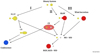 |
Fig. 1. Sketch of the binary evolution paths used in our work. Yellow represents MS stars, red RGB or AGB stars, white WDs, and blue merged objects. |
 (3)
(3)
To account for the fact that the stellar radii change during stellar evolution, we consider their temporal mean for each major evolutionary phase of the star (i.e. MS, RGB and AGB phases), which are derived from PARSEC stellar tracks (Bressan et al. 2012). These are shown in Fig. 2. The criteria for RLOF is set as Rφ(M1, Z) = RL, giving the maximum separation at which the primary star will still fill its Roche lobe, for an evolutionary phase φ:
 (4)
(4)
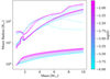 |
Fig. 2. Temporal mean of the stellar radius, derived as a function of mass and metallicity. Solution for MS, RGB and AGB stars are shown, respectively, in solid, dashed and dotted lines |
where Z stands for metallicity.
The stability of the RLOF in channels I and II depends on the critical mass ratio, qcrit. We reconstruct qcrit following the methods described by Ge et al. (2013) for MS stars and Chen & Han (2008) for RGB and AGB stars. Figure 3 shows the reconstructed qcrit as a function of M1 and metallicity for MS, RGB, and AGB donor stars. Based on our definition of mass ratio, RLOF is stable for q > qcrit and unstable for q < qcrit.
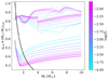 |
Fig. 3. Critical mass ratio as a function of primary mass and metallicity. Solid, dashed and dotted lines represent MS, RGB and AGB, respectively. The black solid curve shows the behavior of qcut(M1). Discontinuities happen because of the changing behavior of the qcrit defining function, and the use of the mean radii. |
The fraction of MS-MS ZAMS binaries that will evolve to a SySt – here considered as a WD-RGB/AGB system – through each channel, is computed from the fraction of systems that satisfy the restrictions for Mthr, q, and a described before.
For channel I, we only considered systems that evolve with a stable RLOF (see Fig. 1), so the fraction of binaries that can evolve to SySt through it is computed as:
 (5)
(5)
where Kq and Ka are re-normalizing functions (that depend on M1 and q) for the ζ(q) and ζ(a) distributions, needed to keep the quantity  as a fraction of fbin* (Eq. (2)). The free parameter fℓ(I) ∈ [0, 1] quantifies our ignorance regarding the fraction of the WD+MS systems formed through channel I that will actually become SySt (see Fig. 1).
For channel II, we have two possibilities, systems where the primary fills its Roche lobe during the RGB or the AGB phases. We produce analogous expressions to compute the fraction of binaries that will evolve through these subchannels and become SySts. For the subchannel II, when there is RLOF on the RGB phase, we have
 (6)
(6)
and when RLOF occurs on the AGB phase,
 (7)
(7)
The only difference between Eqs. (6) and (7) is on the integration limits for a, since AGB stars have mean radii larger than RGB stars (Fig. 2). Each expression is divided in two components, one for the stable and the other for the unstable sub-channel. Here fℓ(II) ∈ [0, 1] is analogous to fℓ(I), but for giant unstable mass transfer.
At last, for channel III, the fraction of SySt formed is given by:
 (8)
(8)
with no free parameter, since we assume that every binary from the initial set – limited by initial amax(M1, q) – will eventually become a SySt through this channel.
The total SySt fraction is then computed considering the sum of all channels, weighted by fbin*. Therefore
 (9)
(9)
where the index i runs over all channels described before.
2.3. The scaling parameter
The previous description can only calculate the fraction of binary systems that evolve into SySts through channels I, II, and III. To determine the actual SySt population, we apply a specific scaling parameter for each galaxy in the sample.
For the MW, the scaling parameter is based on the production density rate of planetary nebulae (PNe), νPN, the observed scale height of symbiotic stars (SySt), hss, the radius of the Galactic disk, RG, and the expected lifetime of the symbiotic phenomenon. This approach is similar to the one used in Kenyon et al. (1993), which assumes that the rate at which PNe are formed is approximately the rate at which low- and intermediate-mass stars form. Thus, the MW scaling parameter is:
 (10)
(10)
Due to the lack of information on the production density rate of PNe, the distribution of SySts, and the properties of LG dwarf galaxies, we use the absolute bolometric magnitude of the galaxy as an estimator of its total stellar content. The bolometric magnitude is calculated using a bolometric correction of −0.2 (Reid 2016). The scaling parameter for these galaxies, 𝒩i, is given by NPNτss/τPN, where NPN is the number of PNe, τPN is their lifetime, and τss is the expected lifetime of the symbiotic phenomenon. The term NPN/τPN approximates the PN formation rate, similar to νPN but not considering a density. Following Buzzoni et al. (2006), NPN can be expressed by ℬτPNLbol, i, where ℬ = 1.8 × 10⁻¹¹ L yr−1 is the specific evolutionary flux. By expressing the luminosity Lbol, i as a function of the absolute magnitude, with the Sun as a reference, the scaling parameter can be written as:
 (11)
(11)
for each dwarf galaxy.
3. Results: Galactic SySt population
In this section, we estimate the SySt population of the MW using both an empirical approach and the model described in Section 2. The empirical approach provides a lower limit, while the theoretical model yields the expected population of MW SySts.
3.1. Empirical limit
Such a limit is set by the observed distribution of SySts. Positions, distances, proper motions and radial velocities (RVs), mainly from Akras et al. (2019) catalog, and the updated version of the New Online Database of Symbiotic Variables (Merc et al. 2019a,b)1 are used in order to infer the empirical limit.
Roughly, 94% (265 of 283) of the confirmed SySt have estimated distances, mostly from Gaia EDR3 (we use the geometric distances; Gaia Collaboration 2016, 2021; Bailer-Jones et al. 2021). By transforming position and distance into galactocentric coordinates, with Astropy (Astropy Collaboration 2018), we produce a Galactic height distribution for the confirmed SySts. This histogram is presented in Fig. 4. A Laplacian distribution is fitted to the data for the computation of the scale height, hss, as being 0.65 kpc – i.e. the Galactic height (ZG) value at which the distribution has fallen to 1/e from its peak value.
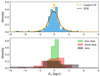 |
Fig. 4. Galactic height distribution for confirmed SySts. Top panel: histogram of the 265 known SySts with distance information, its Gaussian KDE (solid black line), and the fitted Laplacian distribution (dashed orange line). Bottom panel: histograms of galactic heights for the dynamically classified SySts (132 at total). |
Among the confirmed SySts with distance information and the three velocity components estimated, only 132 (47%) have proper motion and RV available from the literature or Gaia. Proper motions are retrieved from Gaia DR3 (Gaia Collaboration 2023), and RVs are provided in the literature (Merc et al. 2019a,b; see Table 1), and in Gaia DR3.
Coordinates, distances, proper motions, and radial velocities of the analyzed stars.
Radial velocities obtained from large-scale surveys do not necessarily represent the γRV (i.e., the RV of the barycenter), in particular if data are obtained only at a single epoch at the unknown orbital phase of the binary. Gaia DR3 produces RVs from observations spanning approximately 1000 days; thus, the measured value probably averages out, at least for the major fraction of SySts, which have orbital periods smaller than 1000 days. Nevertheless, if the binary is unresolved – which is the case of the majority of the SySts –, the measured RV is generally obtained from the cool component. These can be considered in two distinct cases. For S-type SySts, the binary motion significantly impacts the measured RV due to the closer proximity of the components, resulting in higher projected orbital velocities. By analyzing the RVs of the cool components in 47 SySts from our sample, we find that 50% of them exhibit RVs smaller than 7 km/s, and 90% smaller than 10 km/s. If we compare RVs from Gaia DR3 with γRV we note that 50% of them show |RVGaia − γRV| smaller than 2 δRVGaia, being δRVGaia the RV uncertainty in Gaia (see Fig. 5). Thus, accounting for this systematic uncertainty, we raise the RV uncertainties of S-type SySts with RVs from Gaia by a factor of 2. On the other hand, in systems with Mira pulsators (mostly D-type SySts), the cool component pulsations can imply additional variability in RVs of ∼10 km/s (e.g. Hinkle et al. 1989), or even more in some cases. For these systems, where no γRV is measured, we raise their RV uncertainties by ±10 km/s.
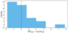 |
Fig. 5. Radial velocity differences for S-type SySt as measured in Gaia DR3 and the literature, normalized by Gaia’s uncertainty (21 SySt). |
Distance estimates from Gaia also warrant careful consideration, given that the astrometric solutions were inferred using single star models. Merc & Boffin (2025) studied the impact of the binary motion on the parallaxes of 500 000 systems, simulated to resemble the known population of SySt and adopting the real Gaia DR3 scanning law. Their results indicate that the ratio of fitted to input parallaxes (ϖfit/ϖ) clusters near unity (see their Figures A.4 and A.5), with no particular dependence on the distance of the system. The vast majority of simulated SySts exhibit ϖfit/ϖ < 1.5. To account for the possible inaccuracies in the parallaxes introduced by the orbital motion, we increased the reported uncertainties of distance estimates from Bailer-Jones et al. (2021) by a factor of 2. Note, that the distance estimates in Bailer-Jones et al. (2021) are not solely based on the parallaxes from Gaia DR3, but use a model of the Galaxy as a prior for the positions of the stars. Also note that increasing the uncertainties does not change the results, since the dynamical classification is based on the velocity components’ median values. Nevertheless, the derived velocity uncertainties are indirectly increased by this approach.
Galactic orbits of the sample stars are integrated over 10 Gyr using galpy (Bovy 2015), to recover the cylindrical velocity components (vr,vφ,vz). These are the equivalent of the (U, V, W) components, but generalized to the global structure of the Milky Way. Thus, vr is the radial velocity (radially on the Galactic plane), vφ is the azimuthal tangent velocity component in the direction of the disk’s rotation, and vz is the velocity component perpendicular to the Galactic plane. These are valid for any position within the Galaxy, not only in the Solar neighborhood, which could be appropriately represented by the UVW velocity system. All of them are given in kilometers per second. To simulate Milky Way’s composed gravitational potential, we superimposed a power spherical potential for the bulge; the Miyamoto–Nagai potential (Miyamoto & Nagai 1975) for the disk; and the Navarro–Frenk–White potential (Navarro et al. 1996) for the halo – included in galpy as MWPotential2014.
With the integrated velocity information, it is then possible to compute the ratio of probabilities of a given SySt to be a part of any major galactic component (i.e. thin disk, thick disk or halo). These probability ratios are expressed as: TD/D, probability of being a part of the thick disk over the probability for the thin disk; and TD/H, probability of being of the thick disk over the probability for the halo (Bensby et al. 2003, 2014; Carrillo et al. 2020; Perottoni et al. 2021). The classification criteria are defined as follows:
-
(a)
TD/D < 0.5 and TD/H > 1 → thin disk;
-
(b)
TD/D > 2 and TD/H > 1 → thick disk;
-
(c)
TD/H < 1 → halo.
From this classification scheme, it is possible to see that objects displaying, at the same time, TD/H > 1 and 0.5 < TD/D < 2, are not classified. These are understood as ‘in between’ the thin and thick disks (Bensby et al. 2014). Applying the criteria above to the SySts with integrated orbits, we retrieve 48 SySts classified as thin disk population (34%), 42 as thick disk (32%), and 32 (24%) as halo population. The remaining 10 SySts have ‘in-between’ dynamics. Figs. 6 and 7 show 1 Gyr of the integrated orbits and the current position of the SySts. Fig. 8, on the other hand, shows the Toomre diagram constructed with the dynamically classified SySt. The high proportion of halo SySts is probably a selection bias, since halo objects have high relative velocities, which are more easily measured.
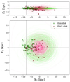 |
Fig. 6. Integrated orbits and current positions of thin (green lines) and thick (pink lines) disk SySts over 1 Gyr. The markers indicate the SySts current position. The interception of the black dashed lines represents the approximate position of the Solar System, for comparison. |
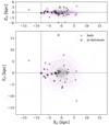 |
Fig. 7. Integrated orbits and current positions of halo and “in-between” (i.e. thin or thick disk dubious objects) SySts. The solid lines show the orbits over 1 Gyr. Markers indicate their current position. The interception of the black dashed lines represents the approximate position of the Solar System, for comparison. |
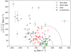 |
Fig. 8. Galactocentric Toomre diagram for confirmed galactic SySts with velocity information. On the horizontal axis we have the circular (azimuthal) velocity component, vφ, and on the vertical axis the squared root of the sum of the squares of the (galactocentric) radial velocity, vr, and vertical velocity, vz. The dashed lines mark constant total velocities (vr2 + vφ2 + vz2)1/2 of 70 and 180 km s−1, centered at the Local Standard of Rest (vφ ≈ 238 km s−1; Reid et al. 2014) for easier visualization. Thus marking the classical boundaries between thin and thick disks. Uncertainties are defined as the standard error, inferred applying a bootstrap analysis (104 drawings for each system). Inferred velocities are displayed in Table 2. |
As a first approximation, we use the distribution of SySts of the thin disk to compute the central SySt number density (n0, the number density at ZG = 0). With the 1σ dispersion ellipsis for thin disk SySts given as
 (12)
(12)
and the thin disk scale height  pc (López-Corredoira & Molgó 2014) we obtained the number density as
 (13)
(13)
where Nin is the number of SySt within the 1σ dispersion region and V1σ is the volume of this region, the σ’s are the standard deviations in x and y directions,  and
and  are the mean XG and YG of the dispersion, and α is a non-dimensional parameter used to fit the dispersion ellipsis to the data. The computed value of n0 was 2.5
 kpc−3. Thus, by integrating the Laplace distribution in ZG and considering the radial and azimuthal SySt distributions as homogeneous, we obtain the number of SySt: 2πRG2hssn0.
Following the fact the dispersion of systems in the thin disk is used to compute n0, the inferred value of n0 can remain roughly the same or increase with the confirmation of new SySt in the disk.
Inferred velocities of the analyzed star, together with the dynamical classification.
Two values are adopted to represent the Galactic disk radius. One of them is the truncation radius, 16.1 kpc (Amôres et al. 2017), which will give the largest possible SySt population, since the stellar density falls with the distance to the galactic center. The other one is 10 kpc, which is five times the scale length of the thin disk and four times the scale length of the thick disk (López-Corredoira & Molgó 2014). This value was chosen due to the fact that it enclosures the Solar System (which is about half the way to the truncation radius), and also because the stellar density has already fallen to a few percent (∼1–2%) of the central value.
From the mentioned parameters, the approximated lower limit for the SySt population in the MW is  for RG = 10 kpc, and
  for RG = 16.1 kpc. Therefore, roughly, we can assume the lower limit is 800–4100 SySt. This value is compatible with the one found by Lü et al. (2006), based on stellar population synthesis, which ranges from 1200 to 15 100 SySt.
3.2. Theoretical expected population
The theoretical results were obtained using the methodology outlined in Section 2. The separation cut, acut(M1, q), determines which evolutionary channels (I, II, or III) are followed by the ZAMS binary systems. We adopt the following values for the scaling parameter terms: (2.4 ± 0.3)×10−12 pc−3 yr−1 for νPN (from Phillips 1989), 5 × 10⁶ yr for τss (from Webbink et al. 1988; Munari & Renzini 1992), 0.65 kpc for hss (see Section 3.1), and {10.0, 16.1} kpc for RG.
The galactic SySt population is computed for a maximum orbital period of log(Pmax) = 6, with Pmax in units of days (Hachisu et al. 1999). For the binary fraction fbin, we use the multiplicity frequency (Duchêne & Kraus 2013), which is a function of M1. Monte Carlo simulations are run considering uniform distributions for fℓ(I), fℓ(II) ∈ [0, 1].
Based on the metallicity distribution in the thin and thick disks of the MW (Yan et al. 2019), we selected two metallicity values for our stellar tracks: Z = 0.006 and Z = 0.014. While there is a significant difference between these values, the impact on our results is negligible (less than 1%). The most noticeable effects are observed only for the stellar models with the lowest metallicities, as in the case of dwarf galaxies. We chose to keep a fix metallicity of 0.014 for the MW.
The SySt population estimate is the median value of all simulations, with uncertainties calculated using a 2σ confidence interval (about 95%). For a Galactic radius of 10 kpc, we obtain an expected SySt population of (53 ± 6)×103, while for a radius of 16.1 kpc (truncation radius), we obtain the upper limit of (138 ± 16)×103. Note that this upper limit should be regarded as an overestimation, since it considers the disk SySt population to be homogeneous up to the galactic truncation radius, which is far from the truth for any stellar population.
4. Results: Local group dwarf galaxies
Due to the limited data availability, we were only able to apply our model in a small number of LG dwarf galaxies. The abundances used, [Fe/H], are given by McConnachie (2012), which, with Z⊙ ≈ 0.02, are converted to metal mass fraction via:
![Mathematical equation: $$ \begin{aligned} Z_i = Z_\odot \times 10^{\mathrm{[Fe/H]}_i}. \end{aligned} $$](/articles/aa/full_html/2025/06/aa51548-24/aa51548-24-eq22.gif) (14)
(14)
About half of our dwarf galaxies’ sample has binary fractions estimated from observations. In the instances where more than one binary fraction is available, we use the range given by the maximum and minimum binary fractions as a third free parameter. For the cases where no information is available, we adopted the range 0.25–0.75 for fbin as a free parameter.
As before, results and uncertainties are obtained from Monte Carlo simulations of the two free parameters described in Section 2 (fℓ(I),fℓ(II)), plus the fbin range when applicable. The expected SySt populations, as a function of MV, are displayed in Table 3 and in Fig. 9.
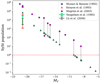 |
Fig. 9. Local Group SySt population as a function of the galaxy’s visual magnitude. Our results, per galaxy, are shown as green triangles, and their uncertainties are not shown because they are about size of the scatter triangles. The red population range, at MV of about −21, is the lower limit range derived from the empirical approach. Data from Munari & Renzini (1992), Kenyon et al. (1993), Yungelson et al. (1995), Magrini et al. (2003), Lü et al. (2006) are plotted for comparison; the dotted lines connect the same galaxies in different works. The red dashed line marks the unity. |
For many galaxies, the derived number of SySts is smaller than one. However, given our assumptions and statistical treatment, these results only imply that we do not expect to find many SySt in these galaxies. An example is the dwarf spheroidal galaxy Draco, for which we derived a null value, but has one SySt confirmed (Akras et al. 2019; Merc et al. 2019a,b).
Another important result is the fraction of ZAMS binaries that evolve through each channel, shown in Table 4. It is clear that channel III is the dominant one and that the difference between channels II RGB and II AGB is considerable. These are direct consequences of the integration limits, which depend on the stellar radii. As shown in Fig. 2, the difference between the mean stellar radii from MS to RGB is much larger than from RGB to AGB. Also, the range from the AGB radii to the equivalent limits in separation for log(P) = 6 is extremely large, which then makes channel III dominate.
5. SNe Ia rate from SySt progenitors
A few hot components in SySt have estimated masses equal or higher than 1 M⊙ (e.g. RS Oph and T CrB; Mikołajewska 2003). Due to the accretion of material from the cool companion, it is reasonable to consider that these objects could approach the Chandrasekhar mass limit (MCh ≈ 1.4 M⊙) in a timescale compatible with the symbiotic phenomenon. By approaching this limit, it is generally accepted that such hot components, if WDs composed mainly by C+O, would experience nuclear instability and, possibly, trigger a thermonuclear explosion disrupting itself, according to the single degenerate scenario (Hillebrandt & Niemeyer 2000). It is expected that this event would be observed as a SN Ia.
The WD composition can be inferred from the simulations, based on the definitions of the channels and an initial-final mass relation (IFMR; Cummings et al. 2018). As a general result, we obtain that about 81% of the WDs in SySt should have a C+O composition, which is explained primarily by the dominance of channel III and also by the IMF (Kroupa 2001) – less massive stars are more abundant. Following the results, a small fraction, 17%, of the SySt WDs would have He dominated composition, represented by channels I and II RGB. And about 2% would be O+Ne WDs.
Restricting ourselves to C+O WDs, we need to know the progenitor masses of such objects, so that it is possible to restrict the parameter space for ZAMS binaries. Following the IFMR from Cummings et al. (2018), we find that such progenitor masses range from ∼0.8 to 6.1 M⊙, while the correspondent WD masses will be within ∼0.55–1.1 M⊙. White dwarfs with masses higher than 1.1 M⊙ would have a O+Ne composition, rather than C+O. However, this is not applicable to all evolutionary channels, since for channels I and II RGB, the primary loses its envelope with a core still completely, or at least mainly, composed by He. Therefore, we also restrict ourselves to channels II AGB and III.
Starrfield et al. (2012) and Hillman et al. (2016) show with detail that RLOF accreting WDs can grow in mass even tough they pass through a series of novae events, ejecting a part of the accreted envelope. More specifically, Hillman et al. (2016) demonstrates that WDs accreting at rates of a few 10−7 M⊙ yr−1 can grow in mass to MCh within a few million years if MWD ≳ 0.8 M⊙, which is compatible with the timescale of the symbiotic phenomenon we are considering in this work. Nevertheless, we note that the lifetime of τss ≈ 5 × 10⁶ yr could be potentially overestimated for a fraction of the SySt population, and we discuss this issue in more detail in Section 6.
According to the IFMR of Cummings et al. (2018) WDs of 0.8 M⊙ are produced by ZAMS stars of 3.3 M⊙, which sets our lower mass limit. From the work of Hachisu et al. (1999) we can also expect that binaries with initial separations in the range of 1500 R⊙ to 40 000 R⊙ shrink to separations of about 800 R⊙, or less, after the evolution of the primary. This means that, when the secondary evolves into a RGB or AGB star, the system can reach considerably high Roche lobe filling factors, producing a RLOF or wind-RLOF evolved binary. Stable mass transfer is needed to allow for WD growing in mass with time. This roughly tells us that the mass of the donor, which is approximately the initial mass of the secondary (Md ∼ M2 = qM1), needs to be smaller than the mass of the WD (Hillman et al. 2016), given by IFMR(M1). Therefore, since the mass ratio has already a lower limit set by qcut(M1), we get the following restriction for mass ratio in the ZAMS
![Mathematical equation: $$ \begin{aligned} q_{\rm cut}(M_1) \le q \le \frac{\mathrm{IFMR}(M_1)}{M_1} < 1,\, M_1\in [3.3,6.1]. \end{aligned} $$](/articles/aa/full_html/2025/06/aa51548-24/aa51548-24-eq23.gif) (15)
(15)
Figure 10 displays such parameter space.
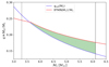 |
Fig. 10. Parameter space for ZAMS systems progenitors of SySt and possible SNe Ia (green filled region). The solid blue line shows the behavior of qcut(M1), and the solid red line that of the upper limit IFMR(M1) / M1 – their interception happens at M1 ∼ 3.6 M⊙. The solid vertical line marks the upper mass limit for C+O WDs of 6.1 M⊙, and the dashed vertical line the lower limit of 3.3 M⊙ for ZAMS stars progenitors of 0.8 M⊙ WDs. |
To derive the expected rate of SNe Ia from SySts we first assume that the rate at which SySts form is very close to the rate they cease to exist – either by triggering a supernova, or by completing their evolution turning into a double WD system or developing a CE phase. From this, it follows that the SySt population in a given galaxy is approximately constant. The rate of SNe Ia from SySt progenitors is thus computed from their expected population, Nss, by limiting the fraction parameter, fss, with the conditions given by expression (15), and thus dividing it by the timescale τss:
 (16)
(16)
Here 𝒩 is the scaling parameter of the corresponding galaxy, and the index ‘i’ runs for channels II AGB and III. It is important to note that we do not take into account possible SNe Ia formed from CE evolution – the core degenerate scenario – or the possible delay times involved in the process (e.g. Soker 2019).
Our results are displayed in the last column of Table 3. The MW has many SNe Ia rates previously published (e.g. 3 × 10⁻³ yr−1, Kenyon et al. 1993 and references therein; (5.4 ± 1.2)×10−3 yr−1, Li et al. 2011;  yr−1, Adams et al. 2013). From the comparison of these works with our result, we suggest that SySts could be progenitors of up to about 1% of the SNe Ia events in the Galaxy. Lü et al. (2009) also estimated a birthrate of symbiotic SNe Ia. They derived a rate between 2.27 × 10⁻⁵ and 1.03 × 10⁻³ yr−1. Our result of (2.8 ± 0.1)×10−5 yr−1 (Table 3) falls close to the lower limit of this range.
Population of SySts and SNe Ia rate from symbiotic progenitors for galaxies in the LG.
Regarding the LG dwarf galaxies in our analysis, the results show that a little more than half of them have symbiotic SNe Ia rate greater than 10−8 yr−1. We would then at least expect hundreds of SNe Ia events in their entire evolution. For the rest of the target dwarfs, timescales for symbiotic SNe Ia (1/rSN) approach the age of the Universe – and add to this fact their null expected population of SySt. Therefore, from our expected values, these galaxies experienced no SNe Ia event, from SySts, in their entire evolution.
6. Discussion
The expected SySt population we derived significantly diverges from the inferences drawn in Munari & Renzini (1992) and Magrini et al. (2003). While the upper limit presented in this work exhibits a similar order of magnitude for the SySt population as in theirs, the mentioned works appear to have substantially overestimated the population. The reason for this comparison with our work, is simply because our upper limit is obtained considering that the disk is homogeneous up to its truncation radius; extremely overestimated. Therefore, we expect the actual population to be much smaller than this limit.
The work of Kenyon et al. (1993) provides a compelling explanation for the overestimation of values in Munari & Renzini (1992). Munari & Renzini (1992) assumes that all binaries with orbital periods between 1 and 10 yr (up to a ∼ 3 AU) evolve into WD–red giant systems. This assumption is overly optimistic, as a significant portion of these binaries is likely to evolve into cataclysmic binary systems. In the present work, binaries within this orbital period range fall into channels I and II. Despite constituting a large fraction of binary systems (Duchêne & Kraus 2013), their contribution to the total SySt population is significantly smaller than that of channel III (Table 4), which comprises the widest binaries. Furthermore, Munari & Renzini (1992) consider all binaries within this orbital period range, including systems with secondary stars that are not massive enough to evolve into giant dimensions within the age of the Universe (Kenyon et al. 1993). Our approach excludes these systems by imposing a threshold mass.
Fraction of SySt formed through each of the defined channels in this work.
Magrini et al. (2003) use K − B colors, distances, and near-IR contributions from young stars in LG galaxies to infer their red giant populations. They assume that 0.5% of red giants are in symbiotic stars. As shown in Figure 9, our derived values and those of Magrini et al. (2003) exhibit a similar slope but a significantly different linear coefficient. The only exception is IC 10, represented by the purple circle close to MV = −17 with an expected SySt population ∼102. In order of magnitude, both works agree for IC 10 SySt population, likely due to its unique status as the only starburst galaxy in the sample (Kim et al. 2009). This starburst activity leads to a higher contribution from young stars, reducing the relative contribution of old stars and consequently diminishing the otherwise inferred SySt number in IC 10.
The expected SySt population we derived closely aligns with that estimated by Kenyon et al. (1993), which is 39 000 SySts. They employ the following expression: 0.5πR2HνPNf1f2f3τss, where R is the Galactic radius, H is the scale height of the disk, νPN is the formation rate of PNe per unit of volume, τss is the timescale of the SySt, and f1, f2, and f3 are fractions regarding binary evolution. While our work is based on a similar expression, there are fundamental differences between these studies. First, it is important to clarify that the evolutionary channels I, II, and III we used differ from the parameters f1 (fraction of binaries with orbital periods within a given range; 1–10 yr and 10–1000 yr), f2 (fraction of binaries that survive the first tidal mass-loss phase as long period systems), and f3 (fraction of binaries with secondaries massive enough to evolve into giant dimensions given the age of the Galaxy), adopted by Kenyon et al. (1993). These authors use τss = 5 × 10⁶ yr for red giant+WD binaries with Porb between 1 and 10 yr, and τss = 1 × 10⁵ yr for Porb between 10 and 1000 yr. In comparison with our ZAMS binaries’ parameters, their approach is equivalent to our channels II RGB/AGB stable and a fraction of the binaries evolving through channel III, accounting for about (2 − 3)×104 SySt, approximately, in our work. Another significant distinction lies in the binary fraction. Kenyon et al. (1993) adopts a fixed binary fraction of 0.5 for stars with masses greater than 0.6 M⊙. In contrast, we employ a variable binary fraction, fbin*, which is derived from the Galactic multiplicity frequency (Duchêne & Kraus 2013) in conjunction with the IMF and mass ratio restrictions (qcut).
Yungelson et al. (1995) considered three channels for the binary population synthesis and derived a Milky Way SySt population range of 3000–30 000, which aligns with our lower limit and expected values. Their channels encompass our channels II (RGB-AGB stable and unstable) and III. However, among the notable differences, is their consideration of primary stars of up to 10 M⊙. Similarly, Lü et al. (2006) tackle the problem by considering the same three channels as Yungelson et al. (1995) with a very similar computational approach. Deriving the range of 1200–15 100 SySt in the Galaxy. An important comparison between our work and Lü et al. (2006), is that all their considered cases agree with the present work that the majority (≳80%) of WDs in SySt is C+O dominated. With their case 4 being the closest, by producing, respectively, 14%, 79%, and 7%, He, C+O, and O+Ne SySt WDs, while ours are 17%, 81%, and 2%, respectively. Nonetheless, our results are consistent with Yungelson et al. (1995) in total number, given that channel I contributes only about 1% to the total population in our work (see Table 4), and with Lü et al. (2006) in WD composition fraction, while not in total number.
It is plausible to argue that not all SySts share the same lifetime. A recent study by Belloni et al. (2024) suggests that SySt such as FN Sgr, with a high Roche lobe filling factor of 0.9, may have a lifetime of approximately 1 × 10⁵ yr. However, in their work the donor in the SySt is more massive than the WD, and the symbiotic evolution culminates in a CE phase. These indicate that the RLOF or wind-RLOF promotes unstable mass transfer between the components in this system. The situation varies from system to system, since stable or unstable mass-transfer depends mainly on the mass ratio and the donor’s envelope structure (Chen & Han 2008). Thus, this timescale does not necessarily apply for stable RLOF/wind-RLOF SySts, which could potentially endure for longer periods, persisting for timescales comparable to the giant’s lifetime. Similarly, Mira D-type SySts, characterized by high mass loss rates, can also be thought to have lifetimes one order of magnitude shorter than the adopted value of τss = 5 × 10⁶ yr (Gromadzki & Mikołajewska 2009). While it is challenging to explicitly account in our work for these two specific SySts types mentioned, we can estimate their maximum impact by making a few simplifying assumptions. If we assume that all SySts with the highest probability of displaying high Roche lobe filling factors (those formed from channels I and II) and all D-type SySt in channel III, ∼17% (based on observational proportions; Akras et al. 2019; Merc et al. 2019a,b), have a lifetime of τss = 1 × 10⁵ yr, while the rest maintain the previous adopted value of τss = 5 × 10⁶, the expected Galactic SySt population becomes 35 × 103. This suggests that, according to the assumptions of this work, the majority of Galactic SySt likely involve less dramatic interactions between components, such as small Roche lobe filling factors, stable RLOF mass transfer, or lower mass loss rates. This is consistent with observations, at least for systems with orbital periods smaller than 1000 days (Mikołajewska 2012), and agrees with Kenyon et al. (1993).
Regarding the dwarf galaxies of the LG, though the limited empirical information does not allow deeper discussions, it is appropriated mentioning the obvious caveats of our model. They are related to the fact we adopted the same mass ratio and orbital period distributions, as well as IMF, as for the Galaxy. Therefore, the results we obtained for their SySt populations should be considered with caution. For instance, if we apply the same scaling parameter used for LG dwarf galaxies (Equation (11)) to the Milky Way, we obtain an estimate of 16 000 SySts. While this value is still within the same order of magnitude as the expected value discussed earlier, it highlights the fundamental differences between the scaling parameters. The parameter for dwarf galaxies is likely to be more uncertain. Comparison with the previous result for the expected SySt population in the Milky Way, shows us that the dwarfs galaxies’ scaling parameter could be underestimated by a factor of 2 or 3.
Our result associated to SNe Ia is based on the channels considered in this work. We selected a subset that would inevitably produce WD-giant systems containing a C+O WD. We also chose the minimum possible WD mass compatible with the potential to reach near-Chandrasekhar mass within the symbiotic lifetime of 5 × 10⁶ yr. For using this lifetime, we restricted the subset to WD-giant systems where the mass-transfer through RLOF/wind-RLOF is expected to be stable. This approach was adopted to calculate the maximum expected contribution of SySt to SNe Ia. The computed rates can be compared with the stellar evolution history of these galaxies to access their compatibility with the [Fe/H] enrichment expected from SNe Ia throughout the galaxy’s chemical evolution. While this is beyond the scope of the current work, it represents an important avenue for future research.
For the Milky Way, several previous studies have estimated the contribution of SySts to SNe Ia. The rates derived are as follows: 10−6 yr−1 (Yungelson et al. 1995); 2 × 10⁻³ yr−1 (Hachisu et al. 1996; Li & van den Heuvel 1997); 2.27 × 10⁻⁵ to 1.03 × 10⁻³ yr−1 (Lü et al. 2009); 6.9 × 10⁻³ yr−1 (Chen et al. 2011); 0.5–1.3 × 10⁻³ yr−1 (Liu et al. 2019). When we compare our SN Ia rate with estimates from these works, and consider the expected number of SySt we derived, we find that up to 1% of SySts could be progenitors of such supernovae through the single-degenerated channel with the conditions specified in this work. If, on the other hand, we are less conservative and consider the upper limit for the SySt population, of ∼1.4 × 10⁵ to compute the rate of SNe Ia, we get 4.5 × 10⁻⁵ yr−1, which still translates into a low contribution of 1.5% to the SNe Ia rate in the Galaxy.
If we consider SySt where mass-transfer can be unstable, thus the considered lifetime should be smaller, τss ∼ 105 yr. In this situation, we cannot make use of the results from Hillman et al. (2016), since they explicit consider stable RLOF mass-transfer for computing the timescales. Following the SySt evolution in Belloni et al. (2024), an analysis regarding CE core-degenerate scenarios for forming SNe Ia (Soker 2019) could be adopted, but it is beyond the scope of this work.
7. Conclusions
From the use of observational data for position, distance, and velocity components of Galactic SySts, we integrated SySt’s orbits and dynamically classified them as thin disk, thick disk, or halo populations. The SySts classified as thin disk objects were used to compute the galactic plane number density as  kpc−3. This value, combined with the derived estimations for the Milky Way’s SySt scale height (0.65 kpc) and disk radius, implied a minimum population of SySts in the MW between 800 and 4100. The, more robust, theoretical procedure, based on binary evolution synthesis, resulted in the expected SySt population of (53 ± 6)×103.
According to the method we adopted in this work, for the Galaxy and the dwarf galaxies in the Local Group (binary evolution synthesis), the SySt population depends on the galaxies bolometric magnitude. The computed populations ranged from a few thousand for the most luminous dwarf galaxies to zero for the fainter ones (Table 3). In any case, as seen in Figure 9, the number of SySts as a function of luminosity (Mv) derived for the MW follows approximately the same trend as for the dwarf galaxies, even though it was computed with a very different scaling parameter. This fact demonstrates the coherence between the methods adopted – empirical and theoretical –, despite their distinct natures.
Regarding SNe Ia progenitors from sigle-degenerate channel, our general conclusion is that SySts cannot be the primary progenitors. This result stems from our analysis of mass growth and the IFMR, which indicates that the vast majority of SySts fall outside the parameter space derived from Hachisu et al. (1999) and Hillman et al. (2016). Nevertheless, we find that a small fraction of SySts could potentially serve as progenitors of SNe Ia (Figure 10). By calculating the formation rate of SNe Ia, we demonstrate that, at most, ∼1% of SNe Ia events in the Galaxy could be originated from SySts. Furthermore, while a few of the considered dwarf galaxies might host symbiotic supernovae, their contribution rates would be so low that we do not expect they could be recorded.
Data availability
Full Tables 1 and 2 are available at the CDS via anonymous ftp to cdsarc.cds.unistra.fr (130.79.128.5) or via https://cdsarc.cds.unistra.fr/viz-bin/cat/J/A+A/698/A155
Acknowledgments
We would like to thank the anonymous referee for the careful reading of the paper and suggestions that helped to significantly improve the methodology and the results displayed here. Authors acknowledge Marco Grossi for discussions about the metallicity and binary fraction of the LG dwarf galaxies, and Luan Garcez for the design of Figure 1. ML’s research is supported by an M.Sc. student’s grant (88887.821757/2023-00) from CAPES – the Brazilian Federal Agency for Support and Evaluation of Graduate Education within the Education Ministry. ML also acknowledges support from FAPERJ (E-26/200.584/2020). DRG acknowledges FAPERJ (E-26/211.370/2021; E-26/200.527/2023) and CNPq (403011/2022-1; 315307/2023-4) grants. HJR-P thanks the Brazilian National Council for Scientific and Technological Development (CNPq) for financial support. The research of JM was supported by the Czech Science Foundation (GACR) project no. 24-10608O. The following software packages in Python were used: Matplotlib (Hunter 2007), NumPy (van der Walt et al. 2011), SciPy (Virtanen et al. 2020) and AstroPy (Astropy Collaboration 2018).
References
- Adams, S. M., Kochanek, C. S., Beacom, J. F., Vagins, M. R., & Stanek, K. Z. 2013, ApJ, 778, 164 [Google Scholar]
- Akras, S., Guzman-Ramirez, L., Leal-Ferreira, M. L., & Ramos-Larios, G. 2019, ApJS, 240, 21 [NASA ADS] [CrossRef] [Google Scholar]
- Allen, D. A. 1984, PASA, 5, 369 [NASA ADS] [CrossRef] [Google Scholar]
- Amôres, E. B., Robin, A. C., & Reylé, C. 2017, A&A, 602, A67 [NASA ADS] [CrossRef] [EDP Sciences] [Google Scholar]
- Astropy Collaboration (Price-Whelan, A. M., et al.) 2018, AJ, 156, 123 [Google Scholar]
- Bailer-Jones, C. A. L., Rybizki, J., Fouesneau, M., Demleitner, M., & Andrae, R. 2021, AJ, 161, 147 [Google Scholar]
- Belczynski, K., & Mikolajewska, J. 1998, MNRAS, 296, 77 [CrossRef] [Google Scholar]
- Belloni, D., Mikołajewska, J., & Schreiber, M. R. 2024, A&A, 686, A226 [NASA ADS] [CrossRef] [EDP Sciences] [Google Scholar]
- Benacquista, M. 2013, An Introduction to the Evolution of Single and Binary Stars (New York: Springer) [Google Scholar]
- Bensby, T., Feltzing, S., & Lundström, I. 2003, A&A, 410, 527 [CrossRef] [EDP Sciences] [Google Scholar]
- Bensby, T., Feltzing, S., & Oey, M. S. 2014, A&A, 562, A71 [NASA ADS] [CrossRef] [EDP Sciences] [Google Scholar]
- Boffin, H. M. J., Hillen, M., Berger, J. P., et al. 2014, A&A, 564, A1 [NASA ADS] [CrossRef] [EDP Sciences] [Google Scholar]
- Bonidie, V., Court, T., Daher, C. M., et al. 2022, ApJL, 933, L18 [Google Scholar]
- Bovy, J. 2015, ApJS, 216, 29 [NASA ADS] [CrossRef] [Google Scholar]
- Brandi, E., Mikołajewska, J., Quiroga, C., et al. 2003, in Symbiotic Stars Probing Stellar Evolution, eds. R. L. M. Corradi, J. Mikolajewska, & T. J. Mahoney, ASP Conf. Ser., 303, 105 [Google Scholar]
- Brandi, E., García, L. G., Quiroga, C., & Ferrer, O. E. 2006, Boletin de la Asociacion Argentina de Astronomia La Plata Argentina, 49, 132 [NASA ADS] [Google Scholar]
- Brandi, E., Quiroga, C., Mikołajewska, J., Ferrer, O. E., & García, L. G. 2009, A&A, 497, 815 [NASA ADS] [CrossRef] [EDP Sciences] [Google Scholar]
- Bressan, A., Marigo, P., Girardi, L., et al. 2012, MNRAS, 427, 127 [NASA ADS] [CrossRef] [Google Scholar]
- Buzzoni, A., Arnaboldi, M., & Corradi, R. L. M. 2006, MNRAS, 368, 877 [Google Scholar]
- Carquillat, J. M., & Prieur, J. L. 2008, Astronomische Nachrichten, 329, 44 [Google Scholar]
- Carrillo, A., Hawkins, K., Bowler, B. P., Cochran, W., & Vanderburg, A. 2020, MNRAS, 491, 4365 [NASA ADS] [CrossRef] [Google Scholar]
- Chen, X., & Han, Z. 2008, MNRAS, 387, 1416 [NASA ADS] [CrossRef] [Google Scholar]
- Chen, X., Han, Z., & Tout, C. A. 2011, ApJ, 735, L31 [NASA ADS] [CrossRef] [Google Scholar]
- Cummings, J. D., Kalirai, J. S., Tremblay, P.-E., Ramirez-Ruiz, E., & Choi, J. 2018, ApJ, 866, 21 [NASA ADS] [CrossRef] [Google Scholar]
- Di Stefano, R., Voss, R., & Claeys, J. S. W. 2011, ApJ, 738, L1 [Google Scholar]
- Duchêne, G., & Kraus, A. 2013, ARA&A, 51, 259 [Google Scholar]
- Dumm, T., Muerset, U., Nussbaumer, H., et al. 1998, A&A, 336, 637 [NASA ADS] [Google Scholar]
- Eggleton, P. 2006, Evolutionary Processes in Binary and Multiple Stars (Cambridge: Cambridge University Press) [Google Scholar]
- Eggleton, P. P. 1983, ApJ, 268, 368 [Google Scholar]
- Fekel, F. C., Hinkle, K. H., Joyce, R. R., & Skrutskie, M. F. 2000a, AJ, 120, 3255 [NASA ADS] [CrossRef] [Google Scholar]
- Fekel, F. C., Joyce, R. R., Hinkle, K. H., & Skrutskie, M. F. 2000b, AJ, 119, 1375 [NASA ADS] [CrossRef] [Google Scholar]
- Fekel, F. C., Hinkle, K. H., Joyce, R. R., & Skrutskie, M. F. 2001, AJ, 121, 2219 [NASA ADS] [CrossRef] [Google Scholar]
- Fekel, F. C., Hinkle, K. H., Joyce, R. R., Wood, P. R., & Lebzelter, T. 2007, AJ, 133, 17 [Google Scholar]
- Fekel, F. C., Hinkle, K. H., Joyce, R. R., Wood, P. R., & Howarth, I. D. 2008, AJ, 136, 146 [Google Scholar]
- Fekel, F. C., Hinkle, K. H., Joyce, R. R., & Wood, P. R. 2010, AJ, 139, 1315 [Google Scholar]
- Fekel, F. C., Hinkle, K. H., Joyce, R. R., & Wood, P. R. 2015, AJ, 150, 48 [NASA ADS] [CrossRef] [Google Scholar]
- Fekel, F. C., Hinkle, K. H., Joyce, R. R., & Wood, P. R. 2017, AJ, 153, 35 [Google Scholar]
- Ferrer, O., Quiroga, C., Brandi, E., & García, L. G. 2003, in Symbiotic Stars Probing Stellar Evolution, eds. R. L. M. Corradi, J. Mikolajewska, & T. J. Mahoney, ASP Conf. Ser., 303, 117 [Google Scholar]
- Gaia Collaboration (Prusti, T., et al.) 2016, A&A, 595, A1 [NASA ADS] [CrossRef] [EDP Sciences] [Google Scholar]
- Gaia Collaboration (Brown, A. G. A., et al.) 2021, A&A, 649, A1 [NASA ADS] [CrossRef] [EDP Sciences] [Google Scholar]
- Gaia Collaboration (Vallenari, A., et al.) 2023, A&A, 674, A1 [NASA ADS] [CrossRef] [EDP Sciences] [Google Scholar]
- Gałan, C., Mikołajewska, J., Iłkiewicz, K., et al. 2022, A&A, 657, A137 [NASA ADS] [CrossRef] [EDP Sciences] [Google Scholar]
- Ge, H., Hjellming, M. S., Webbink, R. F., Chen, X., & Han, Z. 2010, ApJ, 717, 724 [NASA ADS] [CrossRef] [Google Scholar]
- Ge, H., Webbink, R. F., Chen, X., & Han, Z. 2013, in Feeding Compact Objects: Accretion on All Scales, eds. C. M. Zhang, T. Belloni, M. Méndez, & N. Zhang, 290, 213 [NASA ADS] [Google Scholar]
- Geha, M., Brown, T. M., Tumlinson, J., et al. 2013, ApJ, 771, 29 [NASA ADS] [CrossRef] [Google Scholar]
- Griffin, R. F. 1984, The Observatory, 104, 224 [NASA ADS] [Google Scholar]
- Gromadzki, M., & Mikołajewska, J. 2009, A&A, 495, 931 [NASA ADS] [CrossRef] [EDP Sciences] [Google Scholar]
- Gromadzki, M., Mikołajewska, J., & Soszyński, I. 2013, Acta Astron., 63, 405 [NASA ADS] [Google Scholar]
- Hachisu, I., Kato, M., & Nomoto, K. 1996, ApJ, 470, L97 [CrossRef] [Google Scholar]
- Hachisu, I., Kato, M., & Nomoto, K. 1999, ApJ, 522, 487 [NASA ADS] [CrossRef] [Google Scholar]
- Han, Z.-W., Ge, H.-W., Chen, X.-F., & Chen, H.-L. 2020, RAA, 20, 161 [NASA ADS] [Google Scholar]
- Harries, T. J., & Howarth, I. D. 2000, A&A, 361, 139 [NASA ADS] [Google Scholar]
- Harwit, M. 2006, Astrophysical Concepts (New York: Springer) [Google Scholar]
- Hillebrandt, W., & Niemeyer, J. C. 2000, ARA&A, 38, 191 [Google Scholar]
- Hillman, Y., Prialnik, D., Kovetz, A., & Shara, M. M. 2016, ApJ, 819, 168 [NASA ADS] [CrossRef] [Google Scholar]
- Hinkle, K. H., Wilson, T. D., Scharlach, W. W. G., & Fekel, F. C. 1989, AJ, 98, 1820 [Google Scholar]
- Hinkle, K. H., Fekel, F. C., Joyce, R. R., et al. 2006, ApJ, 641, 479 [NASA ADS] [CrossRef] [Google Scholar]
- Hinkle, K. H., Fekel, F. C., & Joyce, R. R. 2009, ApJ, 692, 1360 [Google Scholar]
- Hinkle, K. H., Fekel, F. C., Joyce, R. R., et al. 2019, ApJ, 872, 43 [Google Scholar]
- Hinkle, K. H., Nagarajan, P., Fekel, F. C., et al. 2025, ApJ, 983, 76 [Google Scholar]
- Hunter, J. D. 2007, Comput. Sci. Eng., 9, 90 [NASA ADS] [CrossRef] [Google Scholar]
- Iłkiewicz, K., Mikołajewska, J., Belczyński, K., Wiktorowicz, G., & Karczmarek, P. 2019, MNRAS, 485, 5468 [Google Scholar]
- Jorissen, A., Boffin, H. M. J., Karinkuzhi, D., et al. 2019, A&A, 626, A127 [NASA ADS] [CrossRef] [EDP Sciences] [Google Scholar]
- Kato, M., Hachisu, I., & Mikołajewska, J. 2013, ApJ, 763, 5 [Google Scholar]
- Kenyon, S. J. 2009, The Symbiotic Stars (Cambridge: Cambridge University Press) [Google Scholar]
- Kenyon, S. J., & Garcia, M. R. 1989, AJ, 97, 194 [Google Scholar]
- Kenyon, S. J., Livio, M., Mikołajewska, J., & Tout, C. A. 1993, ApJ, 407, L81 [CrossRef] [Google Scholar]
- Kim, M., Kim, E., Hwang, N., et al. 2009, ApJ, 703, 816 [NASA ADS] [CrossRef] [Google Scholar]
- Kroupa, P. 2001, MNRAS, 322, 231 [NASA ADS] [CrossRef] [Google Scholar]
- Laversveiler, M., & Gonçalves, D. R. 2023, Boletim da Sociedade Astronomica Brasileira, 34, 170 [Google Scholar]
- Li, X. D., & van den Heuvel, E. P. J. 1997, A&A, 322, L9 [Google Scholar]
- Li, W., Chornock, R., Leaman, J., et al. 2011, MNRAS, 412, 1473 [NASA ADS] [CrossRef] [Google Scholar]
- Liu, D., Wang, B., Ge, H., Chen, X., & Han, Z. 2019, A&A, 622, A35 [NASA ADS] [CrossRef] [EDP Sciences] [Google Scholar]
- López-Corredoira, M., & Molgó, J. 2014, A&A, 567, A106 [NASA ADS] [CrossRef] [EDP Sciences] [Google Scholar]
- Lü, G., Yungelson, L., & Han, Z. 2006, MNRAS, 372, 1389 [CrossRef] [Google Scholar]
- Lü, G., Zhu, C., Wang, Z., & Wang, N. 2009, MNRAS, 396, 1086 [CrossRef] [Google Scholar]
- Magrini, L., Corradi, R. L. M., & Munari, U. 2003, in Symbiotic Stars Probing Stellar Evolution, ASP Conf. Ser., 303, 539 [Google Scholar]
- McConnachie, A. W. 2012, AJ, 144, 4 [Google Scholar]
- Meng, X., & Podsiadlowski, P. 2017, MNRAS, 469, 4763 [NASA ADS] [CrossRef] [Google Scholar]
- Merc, J., & Boffin, H. M. J. 2025, A&A, 695, A61 [NASA ADS] [CrossRef] [EDP Sciences] [Google Scholar]
- Merc, J., Gális, R., & Wolf, M. 2019a, Res. Notes Am. Astron. Soc., 3, 28 [Google Scholar]
- Merc, J., Gális, R., & Wolf, M. 2019b, Astron. Nachr., 340, 598 [NASA ADS] [CrossRef] [Google Scholar]
- Mikołajewska, J. 2003, ASP Conf. Ser., 303 [Google Scholar]
- Mikołajewska, J. 2012, Balt. Astron., 21, 5 [NASA ADS] [Google Scholar]
- Mikołajewska, J., & Shara, M. M. 2017, ApJ, 847, 99 [CrossRef] [Google Scholar]
- Mikołajewska, J., Iłkiewicz, K., Gałan, C., et al. 2021, MNRAS, 504, 2122 [CrossRef] [Google Scholar]
- Milone, A. P., Bedin, L. R., Piotto, G., & Anderson, J. 2009, A&A, 497, 755 [NASA ADS] [CrossRef] [EDP Sciences] [Google Scholar]
- Minor, Q. E. 2013, ApJ, 779, 116 [NASA ADS] [CrossRef] [Google Scholar]
- Miyamoto, M., & Nagai, R. 1975, PASJ, 27, 533 [NASA ADS] [Google Scholar]
- Mohamed, S., & Podsiadlowski, P. 2007, in 15th European Workshop on White Dwarfs, eds. R. Napiwotzki, & M. R. Burleigh, ASP Conf. Ser., 372, 397 [Google Scholar]
- Mohamed, S., & Podsiadlowski, P. 2011, in Why Galaxies Care about AGB Stars II: Shining Examples and Common Inhabitants, eds. F. Kerschbaum, T. Lebzelter, & R. F. Wing, ASP Conf. Ser., 445, 355 [Google Scholar]
- Munari, U., & Renzini, A. 1992, ApJ, 397, L87 [NASA ADS] [CrossRef] [Google Scholar]
- Munari, U., Lattanzi, M. G., & Bragaglia, A. 1994, A&A, 292, 501 [Google Scholar]
- Munari, U., Valisa, P., Vagnozzi, A., et al. 2021, Contrib. Astron. Obs. Skalnate Pleso, 51, 103 [Google Scholar]
- Navarro, J. F., Frenk, C. S., & White, S. D. M. 1996, ApJ, 462, 563 [Google Scholar]
- Orio, M., Zezas, A., Munari, U., Siviero, A., & Tepedelenlioglu, E. 2007, ApJ, 661, 1105 [NASA ADS] [CrossRef] [Google Scholar]
- Paczyński, B. 1976, Structure and Evolution of Close Binary Systems, 73, 75 [NASA ADS] [CrossRef] [Google Scholar]
- Pereira, C. B., Baella, N. O., Drake, N. A., Miranda, L. F., & Roig, F. 2017, ApJ, 841, 50 [NASA ADS] [CrossRef] [Google Scholar]
- Perottoni, H. D., Amarante, J. A. S., Limberg, G., et al. 2021, ApJ, 913, L3 [NASA ADS] [CrossRef] [Google Scholar]
- Phillips, J. P. 1989, Proc. 131st Symp. IAU, 425, 442 [Google Scholar]
- Quiroga, C., Mikołajewska, J., Brandi, E., Ferrer, O., & García, L. 2002, A&A, 387, 139 [NASA ADS] [CrossRef] [EDP Sciences] [Google Scholar]
- Reid, W. 2016, in The General Assembly of Galaxy Halos: Structure, Origin and Evolution, eds. A. Bragaglia, M. Arnaboldi, M. Rejkuba, & D. Romano, 317, 83 [Google Scholar]
- Reid, M. J., Menten, K. M., Brunthaler, A., et al. 2014, ApJ, 783, 130 [Google Scholar]
- Reimers, D., Griffin, R. F., & Brown, A. 1988, A&A, 193, 180 [NASA ADS] [Google Scholar]
- Rubele, S., Girardi, L., Kozhurina-Platais, V., Goudfrooij, P., & Kerber, L. 2011, MNRAS, 414, 2204 [NASA ADS] [CrossRef] [Google Scholar]
- Schild, H., Muerset, U., & Schmutz, W. 1996, A&A, 306, 477 [NASA ADS] [Google Scholar]
- Schneider, P. 2015, Extragalactic Astronomy and Cosmology: An Introduction (New York: Springer) [CrossRef] [Google Scholar]
- Smith, V. V., Cunha, K., Jorissen, A., & Boffin, H. M. J. 1997, A&A, 324, 97 [NASA ADS] [Google Scholar]
- Soker, N. 2019, MNRAS, 490, 2430 [Google Scholar]
- Spencer, M. E., Mateo, M., Walker, M. G., et al. 2017, AJ, 153, 254 [NASA ADS] [CrossRef] [Google Scholar]
- Spencer, M. E., Mateo, M., Olszewski, E. W., et al. 2018, AJ, 156, 257 [NASA ADS] [CrossRef] [Google Scholar]
- Stanishev, V., Zamanov, R., Tomov, N., & Marziani, P. 2004, A&A, 415, 609 [NASA ADS] [CrossRef] [EDP Sciences] [Google Scholar]
- Starrfield, S., Iliadis, C., Timmes, F. X., et al. 2012, Bull. Astron. Soc. India, 40, 419 [NASA ADS] [Google Scholar]
- van der Walt, S., Colbert, S. C., & Varoquaux, G. 2011, Comput. Sci. Eng., 13, 22 [Google Scholar]
- Virtanen, P., Gommers, R., Oliphant, T. E., et al. 2020, Nat. Methods, 17, 261 [Google Scholar]
- Webbink, R. F. 1988, in IAU Colloq. 103: The Symbiotic Phenomenon, eds. J. Mikolajewska, M. Friedjung, S. J. Kenyon, & R. Viotti, Astrophys. Space Sci. Lib., 145, 311 [Google Scholar]
- Yan, Y., Du, C., Liu, S., et al. 2019, ApJ, 880, 36 [NASA ADS] [CrossRef] [Google Scholar]
- Yungelson, L., Livio, M., Tutukov, A., & Kenyon, S. J. 1995, ApJ, 447, 656 [Google Scholar]
All Tables
Coordinates, distances, proper motions, and radial velocities of the analyzed stars.
Inferred velocities of the analyzed star, together with the dynamical classification.
Population of SySts and SNe Ia rate from symbiotic progenitors for galaxies in the LG.
All Figures
|
Fig. 1. Sketch of the binary evolution paths used in our work. Yellow represents MS stars, red RGB or AGB stars, white WDs, and blue merged objects. |
| In the text | |
|
Fig. 2. Temporal mean of the stellar radius, derived as a function of mass and metallicity. Solution for MS, RGB and AGB stars are shown, respectively, in solid, dashed and dotted lines |
| In the text | |
|
Fig. 3. Critical mass ratio as a function of primary mass and metallicity. Solid, dashed and dotted lines represent MS, RGB and AGB, respectively. The black solid curve shows the behavior of qcut(M1). Discontinuities happen because of the changing behavior of the qcrit defining function, and the use of the mean radii. |
| In the text | |
|
Fig. 4. Galactic height distribution for confirmed SySts. Top panel: histogram of the 265 known SySts with distance information, its Gaussian KDE (solid black line), and the fitted Laplacian distribution (dashed orange line). Bottom panel: histograms of galactic heights for the dynamically classified SySts (132 at total). |
| In the text | |
|
Fig. 5. Radial velocity differences for S-type SySt as measured in Gaia DR3 and the literature, normalized by Gaia’s uncertainty (21 SySt). |
| In the text | |
|
Fig. 6. Integrated orbits and current positions of thin (green lines) and thick (pink lines) disk SySts over 1 Gyr. The markers indicate the SySts current position. The interception of the black dashed lines represents the approximate position of the Solar System, for comparison. |
| In the text | |
|
Fig. 7. Integrated orbits and current positions of halo and “in-between” (i.e. thin or thick disk dubious objects) SySts. The solid lines show the orbits over 1 Gyr. Markers indicate their current position. The interception of the black dashed lines represents the approximate position of the Solar System, for comparison. |
| In the text | |
|
Fig. 8. Galactocentric Toomre diagram for confirmed galactic SySts with velocity information. On the horizontal axis we have the circular (azimuthal) velocity component, vφ, and on the vertical axis the squared root of the sum of the squares of the (galactocentric) radial velocity, vr, and vertical velocity, vz. The dashed lines mark constant total velocities (vr2 + vφ2 + vz2)1/2 of 70 and 180 km s−1, centered at the Local Standard of Rest (vφ ≈ 238 km s−1; Reid et al. 2014) for easier visualization. Thus marking the classical boundaries between thin and thick disks. Uncertainties are defined as the standard error, inferred applying a bootstrap analysis (104 drawings for each system). Inferred velocities are displayed in Table 2. |
| In the text | |
|
Fig. 9. Local Group SySt population as a function of the galaxy’s visual magnitude. Our results, per galaxy, are shown as green triangles, and their uncertainties are not shown because they are about size of the scatter triangles. The red population range, at MV of about −21, is the lower limit range derived from the empirical approach. Data from Munari & Renzini (1992), Kenyon et al. (1993), Yungelson et al. (1995), Magrini et al. (2003), Lü et al. (2006) are plotted for comparison; the dotted lines connect the same galaxies in different works. The red dashed line marks the unity. |
| In the text | |
|
Fig. 10. Parameter space for ZAMS systems progenitors of SySt and possible SNe Ia (green filled region). The solid blue line shows the behavior of qcut(M1), and the solid red line that of the upper limit IFMR(M1) / M1 – their interception happens at M1 ∼ 3.6 M⊙. The solid vertical line marks the upper mass limit for C+O WDs of 6.1 M⊙, and the dashed vertical line the lower limit of 3.3 M⊙ for ZAMS stars progenitors of 0.8 M⊙ WDs. |
| In the text | |
Current usage metrics show cumulative count of Article Views (full-text article views including HTML views, PDF and ePub downloads, according to the available data) and Abstracts Views on Vision4Press platform.
Data correspond to usage on the plateform after 2015. The current usage metrics is available 48-96 hours after online publication and is updated daily on week days.
Initial download of the metrics may take a while.