| Issue |
A&A
Volume 697, May 2025
|
|
|---|---|---|
| Article Number | A58 | |
| Number of page(s) | 14 | |
| Section | Astronomical instrumentation | |
| DOI | https://doi.org/10.1051/0004-6361/202554055 | |
| Published online | 07 May 2025 | |
The MIRI/MRS Library
II. Pointing-based defringing of unresolved sources
1
Institute of Astronomy, KU Leuven,
Celestijnenlaan 200D,
3001
Leuven,
Belgium
2
Space Telescope Science Institute,
3700 San Martin Drive,
Baltimore,
MD,
21218,
USA
3
UK Astronomy Technology Centre, Royal Observatory,
Blackford Hill Edinburgh,
EH9 3HJ,
Scotland,
UK
4
Department of Physics, Maynooth University,
Maynooth, Co. Kildare,
Ireland
5
Steward Observatory, University of Arizona,
Tucson,
AZ
85721,
USA
6
Institute of Particle Physics and Astrophysics, ETH Zürich,
Wolfgang-Pauli-Str 27,
8049
Zürich,
Switzerland
7
Department of Physics and Astronomy, University of North Carolina,
Chapel Hill,
NC 27599-3255,
USA
★ Corresponding author; This email address is being protected from spambots. You need JavaScript enabled to view it.
Received:
6
February
2025
Accepted:
24
March
2025
Abstract
Context. The Medium Resolution Spectrometer (MRS) of the Mid-InfraRed Instrument (MIRI) on the James Webb Space Telescope (JWST) is affected by interferometric spectral fringing, due to scattering within the detector and dichroic layers. The amplitude of these oscillations on the spectrum can be up to 30%. Correcting them is non-trivial, since the depth and phase of the fringes depend strongly on the illumination pattern and the way the pixels sample it. By default the JWST pipeline uses static fringe flats to divide out the fringes. These flats are representative for a spatially homogeneous extended source, but not for point sources. The significant residuals in the data are removed by using a self-calibrating correction step which can alter physical features in the spectra in a non-systematic way.
Aims. We build on our corrections from Paper I (Gasman et al., 2024, A&A, 688, A226) in this series, to derive a library of detector-based fringe flats for unresolved sources in a nine-point mosaic around all nominal MRS point source dither positions. We provide users with either an absolute or interpolated fringe flat that can correct the fringes without the need for self-calibration, hence mitigating the risk of altering astrophysical features of interest.
Methods. We used the data of 10 Lac from the Cycle 2 calibration programme 3779 to create the library of fringe flats. By removing the continuum and spectral features from the data at the detector-plane level, each of the nine mosaic points around the eight dither positions resulted in a pointing specific fringe flat. By assessing the difference in response between the individual pointings, we found correction factors to bring all the spectra to the same level, and used these to derive a single spectrophotometric calibration curve per band.
Results. The library of fringe flats is able to reduce the remaining power of the fringe frequencies on the detector by up to two orders of magnitude compared to the current pipeline flats tailored to extended sources. This improvement carries over to the residuals in the cube spaxels, where the contrast is reduced from >10% to <1−2%. This becomes less apparent after extracting a spectrum from the cube, where in channel 1 averaging of fringe phases in the current pipeline case can reduce its residual contrast. The spectrophotometric calibration curves have a root-mean squared variation of less than a percent in all bands except bands 4B and 4C, while channels 2 and 3 have a stability within 0.5%. Sources taken without target acquisition (TA) fall outside the mosaic grid, but our correction improves the defringing depending on the source location.
Conclusions. The improvements in fringe residual found are significant on the detector and spectrum-level. The corrections derived here are directly compatible with the current JWST pipeline infrastructure, and work best for unresolved sources observed with TA in one of the nominal point-source dither patterns.
Key words: instrumentation: detectors / methods: data analysis / methods: numerical / infrared: general
© The Authors 2025
 Open Access article, published by EDP Sciences, under the terms of the Creative Commons Attribution License (https://creativecommons.org/licenses/by/4.0), which permits unrestricted use, distribution, and reproduction in any medium, provided the original work is properly cited.
This article is published in open access under the Subscribe to Open model. This email address is being protected from spambots. You need JavaScript enabled to view it. to support open access publication.
1 Introduction
The Medium Resolution Spectrometer (MRS; Wells et al. 2015; Argyriou et al. 2023a) of the Mid-InfraRed Instrument (MIRI; Wright et al. 2023) is an integral field spectrometer on the James Webb Space Telescope (JWST Gardner et al. 2023). Its twelve bands, divided into four channels (1 through 4) with each three sub-bands (‘SHORT’, ‘MEDIUM’, ‘LONG’ or equivalently ‘A’, ‘B’, ‘C’) cover the full wavelength range between approximately 5 and 28 μm. While its performance overall has been phenomenal (Rigby et al. 2023); residual, uncorrected, detector effects must be corrected to reach the photon noise limit. Our goal with the Cycle 2 calibration programme ‘The MIRI/MRS Library’ (Gasman et al. 2023a, PID 3779) is to do just that: addressing detector non-linearity and charge migration Gasman et al. (2024, hereafter referred to as Paper I), detector interferometric fringing, PSF modelling and detector-based extraction, specifically for unresolved sources. For an overview of the programme we refer the reader to Paper I.
The photons incoming at the MIRI/MRS detectors scatter between the detector anti-reflection coating, buried contact, and pixel metallisation, and subsequently interfere with other photons, before being converted into photo-electrons in the infrared-active layer. This results in a sinusoidal-like pattern in the spectral direction of the detectors, and is referred to as fringing. There are three different fringe components present in MRS spectra; two of which originate from scattering in the detectors, and the last from scattering in the dichroic filters present in the MRS optical path. We refer to the latter as the ‘dichroic fringe’. The fringe depth and phase changes across the detectors as a function of detector geometry and wavelength. In Paper I, we demonstrate that the depth of fringing changes as a result of charge migration, caused by a loss in effective responsivity as charge is accumulated at a pixel. Due to a reduced voltage difference between the top and bottom of the active layer (Rieke et al. 2015), the ramps of cumulative charge are non-linear (Morrison et al. 2023). When large contrast occurs between pixels, charge can migrate from the brightest to a less bright pixel, which is referred to as the brighter-fatter effect (BFE, Argyriou et al. 2023b). Since fringes inherently introduce a contrast between pixels, the fringes become less deep for sources reaching up to the full dynamic range of the MRS detectors. The work in Paper I mitigates this crucial aspect of the fringe correction.
Since the fringe pattern is known to change with the way the pupil is illuminated (Argyriou et al. 2020), a static all-purpose fringe flat does not match the fringing in many objects. There are currently three fringe correction steps implemented in the current JWST pipeline (Bushouse et al. 2024): (1) a static fringe flat based on extended illumination (Crouzet et al. 2025), (2) a residual fringe correction based on Bayesian fitting of sinusoids applied on the detector image, and (3) a residual fringe correction in 1D after extracting the spectrum (Kavanagh et al., in prep.). The residual fringe correction is able to remove the residual fringing from objects with non-extended illumination with good performance (Argyriou et al. 2023a), but there is a risk of filtering molecular features if they have a periodicity similar to that of the fringes (Gasman et al. 2023b).
As examined in Argyriou et al. (2020), the fringe depth and phase change depending on what part of the PSF (incoming wavefront) is sampled. Furthermore, Gasman et al. (2023b) demonstrate that the MRS pointing repeatability influences the part of the PSF sampled per pixel, and therefore the resulting fringe pattern. While dividing out the fringe pattern using an unresolved reference source works very well, it only does so if the pointing, and therefore the fringe pattern, is sufficiently repeatable, such that the PSF is sampled in the same way in the detector-space. The relevant MRS local coordinates α and β, representing the on-sky coordinates RA and Dec, are illustrated on the detector in Fig. 1. In the top row of Fig. 2, the change in fringe pattern in band 1A for 10 Lac in PID 3779 for nine different sub-pixel offsets around a single dither position is presented. The top-left panel, where a pixel sampling to the left of the PSF peak is plotted, shows the large difference between point-source fringing (coloured lines) and extended source fringing (black dotted line), and how this deviates between the grid points separated by about 15% of a pixel. In the central panel the fringe pattern on the PSF peak is shown, which should most closely resemble the extended fringe flat due to the illumination on the image slicer being most alike an extended source at that location. However, even in the location that contributes most to the spectral signal the fringes are slightly deeper. This further highlights the need for pointing-based solutions, since statistically even targets observed with target acquisition (TA) can fall up to ∼ 33 mas away from the targeted position (see Paper I).
One of the limitations in the work of Gasman et al. (2023b) is that only a single pointing was available to derive a reference fringe flat. In addition, the reference used was not a deep observation, with low S/N in the longer wavelengths. Using a redder target, such as an asteroid (Pontoppidan et al. 2024), would be a solution to this issue, although its performance would be worse in the shorter wavelengths. In our programme (PID 3779), the 10 Lac observations are relatively deep, reaching up to saturation in channel 1 and parts of channel 2. We assess whether this is sufficient to yield a good S/N for the fringe flats. While the pointing offset requirements for a good correction are likely more stringent in the shortest wavelengths due to the smaller size and undersampling of the PSF (Wells et al. 2015), the longest wavelengths introduce different challenges. At longer wavelengths, the dichroic fringe appears, which is a high-frequency unresolved fringe component. As shown in the bottom row of Fig. 2, it is currently not included in the current pipeline fringe flats, and can therefore only be removed by the residual fringe correction, or a dedicated fringe flat from a reference object.
In this paper, we present the pointing-dependent fringe corrections building on the results from Paper I, and demonstrate the JWST pipeline performance with these new library linearity (Paper I), as well as fringe flats, pixel flats, and response vectors derived in this paper. The paper is structured as follows. In Sect. 2 we discuss the pre-processing steps applied to the PID 3779 data, and other steps required to generate the fringe flats, pixel flats, and spectrophotometric corrections. Sect. 3 focusses on the results from applying the fringe flats, and improvements compared to the current pipeline. The caveats and other considerations for future work are addressed in Sect. 4, and the conclusions are summarised in Sect. 5. In Paper III we will use the tailored pipeline files presented in Paper I and Paper II in order to focus on PSF subtraction at the detector image plane and PSF-weighted detector-based extraction. This work will present a pipeline separate from the JWST pipeline that significantly improves the S/N of spectra for faint unresolved sources, especially in the vicinity of a bright central source. This will be very relevant for extracting spectra of faint brown dwarfs, companions, detecting extended emission, and more.
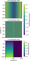 |
Fig. 1 Example of detector coordinate maps for bands 1A (left half of the detector) and 2A (right half of the detector) of the β (top), α (middle), and λ (bottom) coordinates. α and β are analogous to on-sky RA and Dec coordinates. α is ‘along-slice’ on the image slicer and varies within a slice, β is perpendicular to this and varies per slice. The wavelength varies from top to bottom. Note that for the wavelength map we do not show the right half of the detector, since 2A is centred 3 μm further than 1A. |
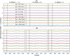 |
Fig. 2 Fringe pattern for nine different PID 3779 pointings around a single dither position in band 1A (top) and 4B (bottom), for one pixel to the left of the PSF peak (left), the central pixel of the PSF (centre), and one pixel to the right of the peak (right). The coloured lines show the pattern from 10 Lac, while the black dotted line shows the extended fringe flat from the current pipeline (Crouzet et al. 2025). The vertical black line highlights where a fringe peak occurs in the extended fringe flat. The Δα values indicate the offset in α coordinate from the central pointing (Δ α = 0). For reference, the pixel size in channels 1 and 2 is 196 mas, and 245 and 273 mas in channels 3 and 4, respectively (Wells et al. 2015). |
2 Methods
2.1 Pre-processing steps
For all current pipeline steps, we applied pipeline version 1.16.1 and pmap 13031. The first step of our code prior to processing the data through the pipeline with our custom files found the centroid of the point source in α and β coordinates. This step required a first estimate for the data that resulted from the first step of the pipeline (CALWEBB_DETECTOR1), which can easily be generated using the current standard pipeline. In Paper I, we present corrections for CALWEBB_DETECTOR1, which were applied to all reference and test data mentioned throughout the work presented here. The reference data were used to generate the fringe flats after applying the aforementioned steps from CALWEBB_DETECTOR1, but before applying any of the corrections described below.
When processing the reference data through the second pipeline module (CALWEBB_SPEC2), most of the standard steps were followed as well. Where mentioned, the standard fringe flat was replaced by the custom files generated here, which we applied prior to running the second pipeline module. When applying the custom fringe reference files, the flat_field reference file was replaced with the file generated as described in Sect. 2.3.2, and the reference files for the photom step replaced by custom files generated as discussed in Sect. 2.3.3. While the current pipeline static spectrophotometric calibration solution was not applied when deriving the custom spectrophotometric calibration files, in all cases the throughput-loss as a function of time (mrs_time_correction) was corrected for Law et al. (2024a). An overview of the pipeline flow and where reference files were replaced with custom input can be found in Fig. 3.
For cube- and spectrum-level tests the standard steps of the third pipeline step (CALWEBB_SPEC3) were applied. Wherever a spectrum was extracted from the cube, the standard aperture size of 2 × FWHM was used, with the appropriate aperture correction factors.
2.2 Generating the fringe flat
Since we aimed to derive fringe flats per pointing, similar to the linearity corrections in Paper I, we derived the different fringe flats from every individual mosaic position and dither of PID 3779. The following steps were applied to yield the cleanest possible fringe flats.
First, the stellar features in the reference star 10-Lac were masked and patched up by fitting a spline between samples. The features were identified automatically. The model of 10 Lac (from the CALSPEC database, Bohlin et al. 2014, 2022) was convolved by the relevant MRS spectral resolution per band (Argyriou et al. 2023a), and features were subsequently identified as σ ≥ 0.6 deviations in channel 3 and band 4A, and σ ≥ 1.5 deviations in all other bands. Additionally, the broader features identified in Law et al. (2024b) were also removed. The clipped wavelengths were projected onto the MRS detector images, and removed if the S/N of the continuum on the detector column was larger than 10, to prevent patching in the background rather than on the source. We detected and clipped spurious outliers from the data as well, with a 3σ offset from the fringe pattern. These clipped detector areas were filled in column-by-column by fitting a spline, based on 50 pixels before and after the clipped area. Bad pixels were replaced in a similar manner. In the longer wavelengths, where the dichroic fringe could not be adequately represented by the spline fit because its period is shorter than the spectral resolution, we made use of the fact that very little variation in fringe pattern seemed to occur in the sub-pixel pointing of the programme. The only major variation occurred due to changes in detector properties over larger offsets (e.g., between the eight nominal dither positions). Therefore, we made use of the observation of the asteroid Athalia in PID 1549 (PI: K. Pontoppidan), which had a high S/N and no spectral features in the patched regions, and spliced in its fringe pattern where features are removed. The results of the feature clipping and replacement method are demonstrated in Fig. 4. Overall, the method seemed to be able to reproduce the fringe pattern well. In channel 4, there was no visible variation in the pattern per dither pointing (see Fig. 2). Since the S/N does decrease in longer wavelengths, we instead averaged the nine pointings around each nominal dither position to derive the fringe pattern.
The reference file should ideally only contain the fringe pattern, and no spectral features or any continuum signal from the star. Therefore, the next step was to divide out the continuum. This step proved to be the most challenging, especially in channels 2 and 3 where the extra beating in the fringe amplitudes was difficult to differentiate from the modulation imposed by the change in the sampling of the PSF and the curvature of the dispersed spectrum in the spectral direction (further referred to as the ‘sampling artefact’). Our initial approach consisted of two sets of filters applied to find the baseline at the centre of the fringe pattern: a Savitzky–Golay filter and a Gaussian filter from scipy (Virtanen et al. 2020). However, while the fringe removal performance was very good in this case, upon examining the FWHM of the detector PSF in each band, we noticed a significant broadening on the top and bottom edges of the detector in channels 2 and 3 due to the sampling artefact not being removed well enough by the continuum fitting. In order to mitigate this issue, we first used a diffraction-limited PSF projected onto the detector in the location of the different 10 Lac exposures to divide out an initial estimate of the PSF shape as sampled by the detector pixels. Since this PSF does not take into account the shape of the SED and is diffraction-limited (which the MRS PSF is not quite due to scattering (Argyriou et al. 2023a)), the remaining fluctuation on the fringe flat continuum was removed using the combination of the Savitzky–Golay and Gaussian filters. Even after removing most of the PSF sampling contribution to the continuum, removing the sampling artefact whilst not including fringing into the continuum proved to be a fine balance. Examples of the resulting continua are presented in Fig. 5.
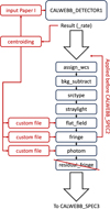 |
Fig. 3 Flowchart of the current standard pipeline and where custom reference files are inserted. |
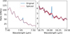 |
Fig. 4 Demonstration of the feature replacement method applied to clean up the fringe flats. On the left the smooth short wavelength fringes are reproduced very well by the spline. On the right, the dichroic fringe in the longer wavelengths cannot be reproduced by the smooth spline, and the patching is done using the asteroid data. |
2.3 Spectrophotometric calibration
2.3.1 Background subtraction
In order to derive the spectrophotometric calibration vector that converts the pixel units of Digital Number (DN) per second to physical units of MJy/sr, the background first had to be subtracted. The programme included two dedicated background observations per band for this purpose. The background was subtracted prior to running CALWEBB_SPEC2. Since first exposures with the MRS tend to be brighter (this is purely a detector electronic effect, see Morrison et al. 2023), the ‘pedestal’ was removed from both the background and 10 Lac reference observations, similarly to the way CALWEBB_SPEC2 corrects for this. This pedestal was determined from the DN/s values in the pixels between the two channels on the detector, which in theory did not contain any on-sky light. In order to create a smooth background for subtraction, each slice in the background observations processed only with CALWEBB_DETECTOR1 was fit with a 2-dimensional polynomial per slice on the detector. These background surfaces had to be subtracted from the 10 Lac reference data after applying the fringe flats generated in Sect. 2.2, since these are used to divide fringes out. If a background was subtracted first, this division would be affected and residual fringes remained.
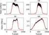 |
Fig. 5 Demonstration of the continuum division for bands 1A, 2A, 3A, and 4A. |
2.3.2 Flat field
The nine sub-pixel pointings around each of the nominal dither positions were all being sampled by the pixels in a slightly different manner. Due to this, the effect of the individual pixel response influenced the total DN/s detected per real flux unit. Normally, the reference files used by the flat_field step should mitigate these discrepancies. However, due to the way these files are derived using on-sky ‘flat’ sources (Law et al. 2024a), small components of noise are also folded into these pixel flats, but components such as pixel response nonuniformity (where the response changes across the surface of a pixel) are averaged out. For unresolved sources with TA, it is not required to have an accurate pixel flat for all parts of the detector, instead only requiring an accurate solution for these small offsets. The rest of the response differences are taken care of by having separate spectrophotometric calibration vectors per dither pattern, as demonstrated in Gasman et al. (2023b). We therefore only needed to reconcile the differences between the nine sub-pixel offsets.
In order to quantify and correct for the difference in response depending on the sub-pixel offset, we extracted separate spectra for each individual pointing, rather than combining the dithers for sampling improvement, as is the standard procedure (Law et al. 2023). These spectra were extracted from cubes with no spectrophotometric calibration applied. The nine points sample the IFU image slicer, and we used the pointing that falls closest to the centre of a slice as a baseline. We did this since the centre of the slice is where we expect the least contribution of vignetting. All other observations were then related to the first in terms of the offset in slice fraction. This was essentially the β-offset divided by the slice width. The correction factor was then defined by dividing the response of the offset pointing by the central pointing. To prevent noise and bad pixels from influencing the correction factors, the reference flats were calculated based on a median value per 50 wavelength bins, and a 2-dimensional second-order polynomial was fit through the cloud of points. This way, all science observations could always be related to an offset value on this polynomial surface, and the relative response value was allowed to vary with wavelength. No trends could be discerned in bands 4B and 4C. We attribute this to the significant drop in signal and increased noise level in the data. Due to the scatter, these bands were not corrected in the flat_field step.
2.3.3 Response correction
For the response correction, we followed the methods in Gasman et al. (2023b) and Law et al. (2024a), including the spectral leak correction. After correcting for the flat field and pixel response differences as described above, we processed the data once more up to the spectral extraction from the cube in the same manner, except this time the four dithers (POSITIVE, NEGATIVE) corresponding to each individual mosaic were combined when building the cube. In addition, no static spectrophotometric correction curve was applied, skipping the photom step in Fig. 3. By following these steps, the correction became compatible with the rest of the current pipeline methods.
Since the response differences from the offsets were already accounted for, the spectrophotometric calibration vector (‘PHOTOM’) was derived from these dither-combined observations. The nine different spectra per dither pattern were averaged together, after which a spline fit, in the same manner as in Law et al. (2024a), was used to remove noise from the subsequent response estimate. The correction factors were then found over the wavelength range by dividing the continuum of the aforementioned 10 Lac model by the spline. The only exception here was channel 1, where the sampling artefact, likely originating from a sub-optimal continuum subtraction in the fringe flat, introduced a 1% variation that differed for the nine mosaics. Therefore, for channel 1 we made separate spectrophotometric calibration vectors depending on the location of the grid point.
Finally, Law et al. (2024a) note that the calibration vector derived from 10 Lac is systematically offset from those of other calibration stars. They derive correction factors to bring the calibration vector up to the same level, and we followed this approach here as well for consistency.
2.4 Interpolating fringe flats
While the calibration programme consists of a finely sampled grid, the chance that a science target lands precisely on one of the grid points on the detector is small. As demonstrated in Fig. 2, the fringes in channel 1 in particular are very sensitive to the exact position of the science target. In this work, we aimed to use the finely sampled grid to examine whether it samples the change in fringes well enough to allow us to combine grid points into a new fringe flat at a new location. We introduce two additional methods to correct for the fringes, aside from a direct division by the fringe flat of the closest grid point. The first we refer to as the ‘mean’. In this case, a weighted mean fringe flat was generated based on the location of the science target relative to the nine grid points per dither position. The flat of each grid point was assigned a weight (wi) based on how close it was to the science target:
 (1)
(1)
The mean flat per dither position is then defined as
 (2)
(2)
where f̄ is the mean flat, wtot the sum of all the weights, and fi the fringe flat of a specific grid point.
The second method is a direct interpolation based on what part of the PSF is sampled by each pixel, similarly to the interpolated non-linearity correction from Paper I. First, the three grid points that have a β position closest to the science observation were found. Next, for the seven brightest detector slices, a point cloud was created from these three fringe flats with three coordinates: the detector row, the offsets in α with respect to the PSF centre of eleven pixels centred around the brightest pixel, and the corresponding value from the fringe flat. For any other science target, the value of the fringe flat per pixel could now be determined by finding the α offset position with respect to its PSF peak, and interpolating within the point cloud. Since this method was less dependent on whether the science target landed within the grid than the weighted mean method, we also tested this method on a target that was not observed with target acquisition. As mentioned in Sect. 1, aside from the illumination pattern, the detector geometry also influences the fringe pattern. Therefore, if the target is too far from the grid in the detector space, this method is not expected to work well either, since the detector geometry will have changed too significantly.
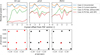 |
Fig. 6 Mean residual power of the fringes in band 1A in the self-calibration case (10 Lac ) and two blue test cases (μCol and δ Umi) for the four different test cases. In channels 3 and 4, where we did not derive BFE-corrected linearity corrections in Paper I, the BFE-corrected case is not included. The position of the observation (red) in detector coordinates α and β with respect to the grid points (black) is presented in the bottom row. |
3 Results
3.1 Performance of the fringe flats
3.1.1 Comparison to current pipeline methods on the detector
In order to assess the performance at the detector image plane level of the fringe flats relative to the current pipeline, we find the fringe residuals as an average of the maximum remaining power from a Lomb-Scargle periodogram using Astropy (Astropy Collaboration 2022) in the fringe frequency range. This is done over the nine pixel columns containing the brightest part of the PSF. We compare the residuals on the detector of a few alternative cases: (1) no fringe correction applied; (2) using the current pipeline extended fringe flat; (3) using the fringe flats derived here, but no BFE correction from Paper I; (4) applying both the BFE correction from Paper I and the fringe flats derived here. This is applied to 10 Lac (self-calibration), but also four test cases that were observed in one of the point-source dither patterns with TA. These test cases include two blue targets, the calibration stars μ Col from PID 4497 (PI: K. Gordon) and δ Umi from PID 1536 (PI: K. Gordon), and two red targets, the asteroid Jena from PID 1549 (PI: P. Pontoppidan) and the young stellar object (YSO) IQ Tau from PID 1640 (PI: A. Banzatti). A summary of the properties of the test targets is given in Table 1. We highlight the most important results below.
Summary of the test targets used in this work, and whether they are brightest in blue or red wavelengths.
As expected, the improvements are best for the self-calibration case 10 Lac, especially in the shorter wavelength channels. As an example, the metrics for band 1A are shown in Fig. 6. The residual power of periodicity is reduced by up to two orders of magnitude. The BFE correction from Paper I also has a significant impact, improving the defringing by an order of magnitude, aligned with our findings in Paper I that the fringe properties are affected by charge migration. The blue test cases μ Col and δ Umi show less extreme improvements, but the fringe flats from this work and BFE correction from Paper I do result in up to an order of magnitude improvement in the short wavelength channels.
The improvements in the longer wavelengths in the 10 Lac and the two red test targets presented in Fig. 7 for band 3A are moderate, which is due to the fact that the longer period fringe does not change as much with PSF sampling in these areas, as also demonstrated in Appendix A. The dichroic fringe has a smaller amplitude, and therefore likely shows a smaller change in power in these cases. However, it is a limiting factor for the detection of many weaker features in these wavelengths, and therefore important to remove. A clear improvement is still observable for all three cases shown in the plot. Overall, the improvement is smaller in channels 3 and 4.
Overall, the correction improves the residual fringe statistics for all test cases and bands on the detector level, compared to the uncorrected case. In general, the defringing performance is also better by up to an order of magnitude compared to the current pipeline. In the next section, we assess the residual on the cube- and spectrum-levels.
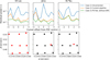 |
Fig. 7 Mean residual power of the fringes in band 3A in the self-calibration case (10 Lac) and two red test cases (Jena and IQ Tau) for the four different test cases. In channels 3 and 4, where we did not derive BFE-corrected linearity corrections in Paper I, the BFE-corrected case is not included. The position of the observation (red) in detector coordinates α and β with respect to the grid points (black) is presented in the bottom row. |
3.1.2 Comparison to current pipeline methods in the cube and cube-extracted spectrum
The pipeline constructs a cube from the different dithers to better visualise the data (Law et al. 2023). In the process, multiple pixels and dithers are combined and the information from the detector is averaged, altering the properties of the fringes. For unresolved sources, a spectrum is then extracted by summing the flux within an aperture in this cube, which further changes the fringes. In order to assess the performance of the library of reference files, we now find the amplitude of the fringe residual in individual cube spaxels and in the summed spectrum after applying the corrections. This is then divided by the continuum flux level in order to find a residual in percent. This method of identifying the fringe residual is the same as in Gasman et al. (2023b). For the cube-level residuals, the residuals are assessed in a square of seven spaxels wide centred on the central spaxel that samples the PSF centroid. The most important results from the cube analysis are presented here. We note that the ideal case is the self-calibration case (10 Lac).
An example of the cube-level performance in the short wavelength ranges is presented in Fig. 8. This figure shows the results for band 1A, but this is similar for other short wavelength bands. As expected from the detector-level measurements, the self-calibration case of 10 Lac and the blue test cases are significantly improved in the cube-level fringe residuals, especially in the shortest wavelengths. the residuals here reduce from >10% in the current pipeline case, to <1−2% in this work. The residuals from the current pipeline flat are smallest closer to the PSF centroid, as this is where the image slicer illumination is most similar to extended source illumination.
The residuals in the longer wavelengths, specifically for band 3A, are shown in Fig. 9. Similarly to the detector-level residuals, the improvements here are more subtle. The residuals are more difficult to assess in IQ Tau, due to the presence of emission lines which can prevent an accurate measurement of the fringe residual (Gasman et al. 2023b), and the metrics appear about the same for the current pipeline and this work. However, subtle improvements can be observed for the 10 Lac and Jena cases, caused by a better removal of the dichroic fringe.
The residuals on the spectrum-level are presented in Fig. 10, where all the test cases are shown in the same plots, and we have added a test case with no TA: CX Tau from PID 1282 (PI: T. Henning, see Table 1 for more details). We first discuss the results of the targets with TA. The improvements in channel 2 are substantial, moving from several percent to sub-percent levels in most cases. The residuals are also improved in channel 3. In channel 4 the improvements are smaller, which in the blue cases is more difficult to measure due to lower signal. The inverse is true for the asteroid Jena, where the signal is very low in the short wavelengths, especially band 1A. In channels 1, 3, and 4 of IQ Tau the methods described in this work show almost no improvement compared to the current pipeline. Similarly to the cube case, the residual fringe measurement becomes more difficult, due to the presence of many densely packed emission lines, which was already shown in to prevent an accurate fringe residual measurement (Gasman et al. 2023b). Interestingly, while the fringe residuals of the test cases mostly improve in channel 1, there are cases where the improvement is unexpectedly small, or the measured fringe residual becomes larger than the residual from the current pipeline fringe flats, which is in strong disagreement with the measurements on the detector and cubes. We address the source of this issue in more detail in Sect. 4.1.
For the test case without TA, applying the fringe flat of the closest grid point does have a mostly positive effect. We observe the largest improvements in band 2A. This test case is also a YSO and therefore contains many emission lines in channels 1, 3, and 4, again limiting our ability to measure the residuals.
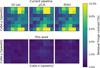 |
Fig. 8 Percent residual fringe contrast for individual cube spaxels in band 1A in the self-calibration case (10 Lac) and two blue test cases (μCol and δ Umi). The top row shows the residuals after only applying the current pipeline flat derived from an extended source, whereas the bottom row presents the residuals after applying both the BFE correction and the fringe flats derived here. |
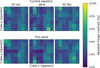 |
Fig. 9 Percent residual fringe contrast for individual cube spaxels in band 3A in the self-calibration case (10 Lac) and two red test cases (Jena and IQ Tau). The top row shows the residuals after only applying the current pipeline flat derived from an extended source, whereas the bottom row presents the residuals after applying both the BFE correction and the fringe flats derived here. |
3.2 Interpolating grid solutions
In the tests above, the fringe flat of the closest grid point was applied to correct for the fringes. In all cases up to the spectrum-level, this results in far smaller residuals compared to the current pipeline fringe flat; up to several orders of magnitude in power on the detector, and from >10% to <1−2% in the cube spaxels. However, especially in the short wavelengths, the large variation in fringe pattern between pointings means that the fringes are not perfectly corrected for when using a closest grid point. These bands would therefore benefit from a custom fringe flat tailored to where the science target lands on the detector. We test the two methods described in Sect. 2.4 for μCol, a target with TA where the grid method seems to perform worst in the spectrum level compared to the current pipeline, and the target without TA, CX Tau. For the former we only test this in the shortest wavelengths, since the grid solution works well enough already in the longer wavelengths due to smaller variations. For the latter, this is done in all channels except for channel 4, where we obtained no spatial information since we averaged the grid points to generate one fringe flat. We note that the weighted mean method cannot be applied to the target without TA, since it falls outside the grid.
The results for these tests are also included in Fig. 10. For μ Col, the blue target with TA, the weighted mean performs similarly to using the grid directly. Very small improvements can be observed in bands 1B and 1C, whereas it performs slightly worse in 2B and 2C. However, these differences are visually indistinguishable. On the other hand, the direct interpolation method overall performs similarly to the grid, or better. In terms of alternative methods, it seems to be the better option compared to the weighted mean.
In the case of CX Tau, no difference can be observed in the residual metric when applying the interpolation method as opposed to the direct grid division. Either the improvements are on a similar level as for μ Col, but unobservable due to the features in the spectrum, or there is no improvement at all. Regardless, the interpolation method does not do worse in this case.
3.3 Comparison to residual fringe correction
The comparison of a dedicated reference fringe flat to all the current pipeline fringe correction methods, including the residual fringe correction, was done more extensively in Gasman et al. (2023b). That work demonstrates that the residual fringe correction is able to bring down residual fringing to sub-percent levels, but has inherent limitations due to its self-calibrating nature. Since it is essentially a frequency filter, its excellent defringing performance is expected. However, a downside of the frequency filtering approach is that some molecular features contain similar frequency signatures, and can be mistaken for fringes by the algorithm. It can therefore change the relative strength and shape of molecular features in a non-systematic manner. In that work, this was demonstrated for CO in a star. Because it is sometimes difficult to ascertain what exactly has been removed or changed by the residual fringe correction, in the above tests we opted for an ‘apples to apples’ comparison approach, only comparing to the current pipeline static fringe flat. Static corrections allow for easier traceability of spurious features. However, to further demonstrate the potential disadvantages of the residual fringe correction, we take the example of the very molecule rich YSO test object IQ Tau. In one case we apply the complete list of current standard pipeline correction steps, whereas in the other we only apply the methods introduced here.
The resulting spectra are presented in Fig. 11. The top panel shows the wavelength region with emission from CO. The spectrum reduced with the residual fringe correction has slightly different relative power between emission features. This difference, though subtle, can make a difference in the excitation properties derived from such a spectrum. Furthermore, in the bottom panel a region of the spectrum typically strongly affected by the dichroic fringe is shown. In this case, the current pipeline reduction clearly shows considerable extra high-frequency residuals in the spectrum, that do not appear in the reduction using the dedicated reference files. The dichroic fringe is difficult to remove using the residual fringe correction, especially in the presence of a forest of other emission features. In cases like these, the static, dedicated the reference files of our library have a clear advantage. However, this becomes less apparent for stars with less line rich spectra, such as the test cases in Gasman et al. (2023b). In those cases, less care about molecular features is required, and the current pipeline with residual fringe correction perform well.
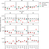 |
Fig. 10 Percent residual fringe contrast on the extracted spectra of 10 Lac, μ Col, δ Umi, Jena, IQ Tau, and CX Tau, identified per individual band. Four different reduction methods are shown: using only the current pipeline fringe flat, using the BFE correction and fringe flats derived here, using the BFE correction with interpolated fringe flats, and using the BFE correction with a weighted mean of the fringe flats. |
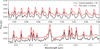 |
Fig. 11 Spectrum of the test case IQ Tau, when applying the current pipeline static fringe flat and residual fringe corrections (black), and only the static correction methods introduced in this work (red). |
4 Discussion
4.1 Discrepancies in fringe residuals in the cube
In Sect. 3.1.2 the fringe residuals on the spaxel level are consistent with the improvements on the detector level, where the current pipeline flat performs significantly worse, especially in the sensitive short wavelength regions. However, after moving to the spectrum level, this difference seems to largely disappear, especially in channel 1. This may appear contradictory, but this is actually a logical consequence of the large fringe phase variations across the PSF in channel 1, which can be anticorrelated across the PSF (see for instance Fig. 18 in Argyriou et al. 2020). When summing different cube spaxels with fringes offset in phase, they average out and result in a much cleaner looking spectrum. This effect is demonstrated in Fig. 12, where the spectra of two bright spaxels in the cube are plotted. It is clear that the fringe residual in the spaxel level is indeed much larger for the current pipeline flat than for the grid flats presented here. However, the fringes left in the cubes resulting from the current pipeline are almost exactly out of phase between the two spaxels. Therefore, when summing the flux in an aperture, the fringes cancel each other out and the residual is reduced to a smaller amplitude. The residuals after applying the grid correction are already much smaller, but more in-phase than the current pipeline. Summing the spaxels in this case does not reduce the amplitude, but may actually increase it. While summing the spaxels may appear to make the fringes disappear in the current pipeline case, this does not mean that all observations benefit from this effect, due to differences in pointing, and have consistent fringe residuals. This is visible for the two blue test cases, where for μ Col the discrepancy in band 1B is much larger than for δ Umi (see Fig. 6).
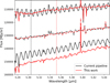 |
Fig. 12 Spectra from two single spaxels (solid lines), and the sum of 5×5 spaxels divided by 7 to display the spectrum in the centre (dash-dotted line). The black vertical line indicates a fringe peak in the brightest spaxel of the current pipeline cube, which does not correspond to a fringe peak in the less bright spaxel due to a phase shift. The red vertical line corresponds to a fringe peak in the brightest spaxel of the grid correction instead. |
4.2 Caveats and future improvements
4.2.1 Continuum subtraction
Two improvements made to the method of deriving the fringe flats compared to Gasman et al. (2023b), include a better and more consistent continuum subtraction, and the removal of spectral lines. We already noted above that the continuum subtraction is not perfect, and may still contain a part of the sampling artefact. This results in larger inconsistencies between spectrophotometric calibration curves in channel 1, and a substantial broadening of the PSF at band edges in channel 2. We expect that this can be improved further by a better PSF model in the cube that can be projected onto the detector. The development of such a model at the cube-level is already in progress is already in progress in Patapis et al. (in prep.).
4.2.2 Feature removal
The removal of spectral lines was possible because we were able to patch the spectrum by fitting splines or by patching in the asteroid observation. However, four broad lines were identified in Law et al. (2024b), that are not present in the model used to identify the spectral lines and flux of the object. Three of these are on the long wavelength detector, where the change in fringe pattern with pointing is less extreme, and the asteroid observation could be used. However, in the short wavelengths this is not possible due to the variation of the fringes between pointings. Because of the width of the line, it was not possible to patch this area with a spline. We therefore note the caveat that a weak [Ne VI] emission line ranging from 7.6 to 7.7 μm may affect the spectra corrected with the methods presented here.
4.2.3 Recommendations for future calibration programmes based on the PID 3779 observing strategy
Unless the science target falls almost perfectly on the grid in the detector space, the fringe corrections, especially in channel 1, may still be sub-optimal when examined in the resulting spectrum. This is especially apparent when comparing the fringe residuals of μ Col and δ Umi in channel 1, where is δ Umi generally located closer to a grid point, especially in the α coordinate (see Fig. 6). In Appendix A, we assess the variation of the fringe residuals as a function of offset in more detail. From Fig. A.1, it becomes clear that the residuals in channel 1 are most sensitive to offsets, especially in the α-direction. Therefore, the resulting performance of the flats is considerably worse for μ Col than for δ Umi. Interpolation of flats is able to improve this somewhat, but not sufficiently to yield a consistent defringing performance. Therefore, it appears that an even finer grid is required to properly correct the short wavelengths. Initially we anticipated the 30 mas grid to be sufficient to sample the wavefront enough for the changes to become linear. Extra observations halfway between the current grid, in other words resulting in a spacing of 15 instead of 30 mas, are advised for channels 1 and 2. An alternative would be to extract spectra from both the reference and science target without applying any fringe corrections and dividing the two in the spectrum level. By doing so, one can cross-correlate and shift fringes to minimise the residuals. While this approach would be advantageous for users of the cube-extracted spectra, it is less straightforward to apply on the detector.
Finally, we note that, similar to Paper I, the noise in the longer wavelength bands results in a sub-optimal correction. Especially bands 4B and 4C are affected by this. As with the non-linearity, this can be corrected for by using a similar set of observations targeting a red object. One such example would be an asteroid. Contrary to the short wavelengths, the grid spacing used in this programme appears sufficient to correct the fringes in a wide range of spectra. The variation in the main fringe component is not noticeable on the scale of the offsets presented here, but that of the dichroic fringe is. However, Fig. A.1 indicates that this becomes noticeable at offsets of ∼ 50 mas or larger, which is well outside the expected pointing accuracy of targets observed with TA. Therefore, the recommendation for long wavelengths is to observe a red target, such as an asteroid, in the same grid as used by this programme.
The recommendations given here are solely to overcome issues of the pointing accuracy and low S/N of the star at long wavelengths. For as far as we are currently aware, fringes are not subject to temporal variations.
5 Conclusion
In this work, we have built upon the results from Paper I to address the fringing issue in the MIRI/MRS, and create a full set of reference files compatible with the current JWST pipeline infrastructure. This set-up, that uses the current JWST pipeline, is specifically applicable to unresolved sources, observed with TA in one of the nominal point-source dither patterns.
We use the nine-point mosaic around each nominal point source dither position in PID 3779 to derive a grid of fringe flats, flat fields, and spectrophotometric calibration files. The fringe flats improve the residual power of the fringes on the detector by up to several orders of magnitude for the self-calibration case, when compared to the current pipeline flats. Even for the blue and red reference targets, this improvement is up to an order of magnitude. The BFE correction from Paper I also has a substantial influence on the performance of the fringe correction, demonstrating that any kind of contrast causes variations between different data. An improvement in fringe contrast compared to the current pipeline flats of >10% down to <1−2% is observed in the cube spaxels. This improvement becomes smaller and less consistent when moving to the 1D-extracted spectrum residuals, due to averaging of fringe phases in the current pipeline case.
The variation of fringe depth and phase with pointing is largest in the shorter wavelengths, and a finer grid of 15 mas may be necessary here for more consistent performance. The longer wavelength bands are more consistent with extended fringes, although more variation is observed in the dichroic fringe. A red target with a smooth continuum (such as an asteroid) observed in the same 30 mas grid would improve the performance of the reference files in channel 4.
For Paper III, our goal is to enable detector-based spectral extraction. Therefore, we are most interested in improving the PSF characterisation and the fringe residuals on the detector level. Especially in this case, we have proven that the grid performs exceptionally well compared to the current pipeline flat. The work presented here and Paper I are essential for improving the sensitivity of the MIRI/MRS and the reach the photon-noise limit.
Data availability
The code to run the pipeline with the reference files generated in Paper I and here are available on Github: https://github.com/DannyG20/MIRI-MRS-Library-Pipeline.
Acknowledgements
This work is based on observations made with the NASA/ESA/CSA James Webb Space Telescope. The data were obtained from the Mikulski Archive for Space Telescopes at the Space Telescope Science Institute, which is operated by the Association of Universities for Research in Astronomy, Inc., under NASA contract NAS 5-03127 for JWST. These observations are associated with programs #3779, #4497, #1536, #1549, #1640, and #1282. Danny Gasman, Ioannis Argyriou, thank the European Space Agency (ESA) and the Belgian Federal Science Policy Office (BELSPO) for their support in the framework of the PRODEX Programme. P.J.K. acknowledges financial support from the Science Foundation Ireland/Irish Research Council Pathway programme under Grant Number 21/PATH-S/9360. The work presented is the effort of the entire MIRI team and the enthusiasm within the MIRI partnership is a significant factor in its success. MIRI draws on the scientific and technical expertise of the following organisations: Ames Research Center, USA; Airbus Defence and Space, UK; CEA-Irfu, Saclay, France; Centre Spatial de Liége, Belgium; Consejo Superior de Investigaciones Científicas, Spain; Carl Zeiss Optronics, Germany; Chalmers University of Technology, Sweden; Danish Space Research Institute, Denmark; Dublin Institute for Advanced Studies, Ireland; European Space Agency, Netherlands; ETCA, Belgium; ETH Zurich, Switzerland; Goddard Space Flight Center, USA; Institute d‘Astrophysique Spatiale, France; Instituto Nacional de Técnica Aeroespacial, Spain; Institute for Astronomy, Edinburgh, UK; Jet Propulsion Laboratory, USA; Laboratoire d’Astrophysique de Marseille (LAM), France; Leiden University, Netherlands; Lockheed Advanced Technology Center (USA); NOVA OptIR group at Dwingeloo, Netherlands; Northrop Grumman, USA; Max-Planck Institut für Astronomie (MPIA), Heidelberg, Germany; Laboratoire d’Etudes Spatiales et d’Instrumentation en Astrophysique (LESIA), France; Paul Scherrer Institut, Switzerland; Raytheon Vision Systems, USA; RUAG Aerospace, Switzerland; Rutherford Appleton Laboratory (RAL Space), UK; Space Telescope Science Institute, USA; Toegepast- Natuurwetenschappelijk Onderzoek (TNO-TPD), Netherlands; UK Astronomy Technology Centre, UK; University College London, UK; University of Amsterdam, Netherlands; University of Arizona, USA; University of Bern, Switzerland; University of Cardiff, UK; University of Cologne, Germany; University of Ghent; University of Groningen, Netherlands; University of Leicester, UK; University of Leuven, Belgium; University of Stockholm, Sweden; Utah State University, USA. A portion of this work was carried out at the Jet Propulsion Laboratory, California Institute of Technology, under a contract with the National Aeronautics and Space Administration. We would like to thank the following National and International Funding Agencies for their support of the MIRI development: NASA; ESA; Belgian Science Policy Office; Centre Nationale D’Etudes Spatiales (CNES); Danish National Space Centre; Deutsches Zentrum fur Luft-und Raumfahrt (DLR); Enterprise Ireland; Ministerio De Economiá y Competividad; Netherlands Research School for Astronomy (NOVA); Netherlands Organisation for Scientific Research (NWO); Science and Technology Facilities Council; Swiss Space Office; Swedish National Space Board; UK Space Agency. We take this opportunity to thank the ESA JWST Project team and the NASA Goddard ISIM team for their capable technical support in the development of MIRI, its delivery and successful integration.
Appendix A Variation of fringes with offset
We are able to generate fringe flats for all different pointings, except for channel 4 where we average the fringe flats to improve the noise performance. Using these, we can assess the change in fringe flat performance with offset between the science and reference targets. In order to do so, we apply all nine fringe flats to all nine mosaic points, and we repeat that for each of the eight dithers. We then compute the residuals in the column containing the PSF peak and one neighbouring column on each side of the peak. These residuals are defined as the average of the maximum remaining power from a Lomb-Scargle periodogram using Astropy (Astropy Collaboration 2022) over the three pixel columns, in the fringe frequency range. The value of the power is then normalised by the residual power in the point where the flat is applied to the data from which it was derived (self-calibration) where the fringes are perfectly removed. These maximum residual values are plotted as a function of offset in detector coordinates α and β in Fig. A.1.
Based on the colour scale corresponding to each channel, it becomes clear that the largest residuals occur for channel 1, when the offset becomes too large. This dependency is also most clearly visible in these data, where especially bands 1B and 1C clearly demonstrate a trend between the decrease in defringing performance and offset. The performance of the files seems to be most dependent on the offset in α, however, the β-offset is not of negligible influence. While the influence of offset becomes less important in channel 2, it is still clear that larger offsets do result in larger fringe residuals.
Interestingly, channel 3 in the bottom row of Fig. A.1 shows a pattern where larger residuals occur only in either positive or negative α-offsets. In channel 3, the change in the longer period fringe component on the scale of the mosaic is negligible, as also demonstrated in Fig. 2, and this component is adequately removed. However, in these wavelengths the dichroics fringe, which does seem to depend on the sampling of the PSF. We demonstrate this in Fig. A.2, where we show only one nine-point mosaic set. In bands 3A and 3B, the largest residuals occurred for positive Δα. We therefore take the observation with the smallest α-coordinate, and use that as our reference. In the case of band 3C, the largest residuals occurred for negative Δα, and as such we used the observation with the largest α-coordinate as the reference. The self-calibration case is included, which results in a straight line. We can see that the high-frequency pattern indeed becomes more pronounced towards larger offsets, whilst the low-frequency fringe component is perfectly removed. This indicates that at longer wavelength ranges, the offset only limits the capability of the correction to remove the dichroic fringe.
The variation in fringe pattern in channels 1 and 2 are the largest, which is also demonstrated by the fact that the current pipeline flat is not capable of consistently reducing the fringe amplitude to percent and sub-percent levels. Figure A.1 shows that a 30 mas offset is enough to cause the resulting spectrum to be significantly affected by fringes, and the residuals in our test cases further demonstrate this. The targets were within 15 mas of a grid point, yet the resulting fringe residual on the spectrum level could still reach up to a percent. However, it appears that band 2C is already less affected by this. The sensitivity of the fringe pattern to the exact pointing changes with wavelength, where fringe patterns in the shorter wavelengths vary more quickly. Since the fringes of a fully extended source are consistent between detector columns, unlike those of an unresolved source, it is likely that the closer the illumination is to being fully extended, the less sensitive the fringe pattern becomes to the way the illumination is sampled. Therefore, in shorter wavelengths the PSF is smaller and the background low, meaning the illumination diverges most from being fully uniform and extended. The longer the wavelength, the larger the PSF and the higher the background, which may be the cause of the fringes becoming more consistent.
This is visible in the longer period fringe in channels 3 and 4, which is consistent with the current pipeline flat and well-corrected by both methods. Interestingly, this does not seem to hold for the dichroic fringe, which we observe to change with offset in Figs. 2 and A.2. The reason for this is currently not clear.
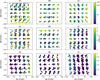 |
Fig. A.1 Change in fringe residual as a function of offset between ‘science’ and ‘reference’ targets. |
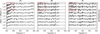 |
Fig. A.2 Change in residual fringing in channel 3 when applying increasingly offset fringe flats. The order in which the different observations are plotted is in accordance with the findings from Fig. A.1; the difference in α offset becomes larger towards the top of the plot. The red boxes indicate parts with a clear residual from the dichroic fringe. |
Appendix B Performance of the spectrophotometric calibration
We will now assess the quality of the spectrophotometric calibration. After applying the custom pixel flat and spectrophotometric calibration to the individual exposures, the four dithers per mosaic are combined and the spectra are extracted. The spectrophotometric calibration curves are based on an average of all these different exposures, and using this we can define a rootmean squared (RMS) per band, to assess the performance of the pixel flats, and the stability of the spectrophotometric calibration within the grid points. The results of this are shown in Fig. B.1.
The RMS of the spectrophotometric calibration curves are well within 1% for almost all bands, and even less than 0.5% for band 1C, channels 2 and 3, and most of band 4A. This means that the pixel flat function is able to bring all observations to the same level with great accuracy. The main outliers here are bands 4B and 4C, which, as expected, have larger variations due to noise because of the low stellar signal in these wavelengths. As discussed in Sect. 2.3.3, we are unable to derive good pixel flats for these bands due to the large scatter, which further reduces the consistency between the mosaic points. Furthermore, the residuals of channel 1 show an up to 1% RMS due to differences in the sampling artefact between the mosaic points. The latter also results in a visible sampling artefact in the spectrum for observations that do not land exactly on a grid-point, most notable μ Col.
In Fig. B.2 the percent differences in flux level between band overlap regions are shown for the two blue and two red test targets. The current pipeline already performs well in this metric, with the flux in overlap regions varying around 1%. With the methods presented here, we mostly match these numbers. Similarly to the fringing performance, the main improvements are observed in the shortest wavelengths, particularly channel 1. The only exception to the 1% overlap accuracy is the asteroid Jena, which naturally has large temporal flux variations due to rotations. Since the sub-bands are observed simultaneously, it naturally follows that the overlap in sub-bands B-C is similar and smallest for all channels, whereas the overlap regions of subbands A-B and C-A are also at a similar level for the different channels. This is the same for both the current pipeline and this work, therefore we conclude that the performance for the current pipeline and the methods presented here is similar.
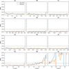 |
Fig. B.1 RMS of the spectrophotometric calibration curves, based on the differences between the nine different dither-combined spectra. The performance in bands 4B and 4C are considerably worse due to low signal in the calibration star 10 Lac. |
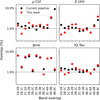 |
Fig. B.2 Percent difference in flux level between overlap regions of the different bands. |
References
- Argyriou, I., Wells, M., Glasse, A., et al. 2020, A&A, 641, A150 [NASA ADS] [CrossRef] [EDP Sciences] [Google Scholar]
- Argyriou, I., Glasse, A., Law, D. R., et al. 2023a, A&A, 675, A111 [NASA ADS] [CrossRef] [EDP Sciences] [Google Scholar]
- Argyriou, I., Lage, C., Rieke, G. H., et al. 2023b, A&A, 680, A96 [NASA ADS] [CrossRef] [EDP Sciences] [Google Scholar]
- Astropy Collaboration (Price-Whelan, A. M., et al.,) 2022, ApJ, 935, 167 [NASA ADS] [CrossRef] [Google Scholar]
- Bohlin, R. C., Gordon, K. D., & Tremblay, P. E., 2014, PASP, 126, 711 [NASA ADS] [Google Scholar]
- Bohlin, R. C., Krick, J. E., Gordon, K. D., & Hubeny, I., 2022, AJ, 164, 10 [NASA ADS] [CrossRef] [Google Scholar]
- Bushouse, H., Eisenhamer, J., Dencheva, N., et al. 2024, https://doi.org/10.5281/zenodo.14153298 [Google Scholar]
- Crouzet, N., Mueller, M., Sargent, B., & Lahuis, F., 2025, A&A, in press https://doi.org/10.1051/0004-6361/202452903 [Google Scholar]
- Gardner, J. P., Mather, J. C., Abbott, R., et al. 2023, PASP, 135, 068001 [NASA ADS] [CrossRef] [Google Scholar]
- Gasman, D., Argyriou, I., Glasse, A., et al. 2023a, The MIRI MRS Library (USA: JWST Proposal. Cycle 2), ID. #3779 [Google Scholar]
- Gasman, D., Argyriou, I., Sloan, G. C., et al. 2023b, A&A, 673, A102 [NASA ADS] [CrossRef] [EDP Sciences] [Google Scholar]
- Gasman, D., Argyriou, I., Morrison, J. E., et al. 2024, A&A, 688, A226 [NASA ADS] [CrossRef] [EDP Sciences] [Google Scholar]
- Law, D. R. E., Morrison, J., Argyriou, I., et al. 2023, AJ, 166, 45 [NASA ADS] [CrossRef] [Google Scholar]
- Law, D. R., Argyriou, I., Gordon, K. D., et al. 2024a, arXiv e-prints [arXiv:2409.15435] [Google Scholar]
- Law, D. R., Hawcroft, C., Smith, L. J., et al. 2024b, arXiv e-prints [arXiv:2410.05469] [Google Scholar]
- Morrison, J. E., Dicken, D., Argyriou, I., et al. 2023, PASP, 135, 075004 [NASA ADS] [CrossRef] [Google Scholar]
- Pontoppidan, K. M., Salyk, C., Banzatti, A., et al. 2024, ApJ, 963, 158 [NASA ADS] [CrossRef] [Google Scholar]
- Rieke, G. H., Ressler, M. E., Morrison, J. E., et al. 2015, PASP, 127, 665 [NASA ADS] [CrossRef] [Google Scholar]
- Rigby, J., Perrin, M., McElwain, M., et al. 2023, PASP, 135, 048001 [NASA ADS] [CrossRef] [Google Scholar]
- Virtanen, P., Gommers, R., Oliphant, T. E., et al. 2020, Nat. Methods, 17, 261 [Google Scholar]
- Wells, M., Pel, J. W., Glasse, A., et al. 2015, PASP, 127, 646 [NASA ADS] [CrossRef] [Google Scholar]
- Wright, G. S., Rieke, G. H., Glasse, A., et al. 2023, PASP, 135, 048003 [NASA ADS] [CrossRef] [Google Scholar]
All Tables
Summary of the test targets used in this work, and whether they are brightest in blue or red wavelengths.
All Figures
|
Fig. 1 Example of detector coordinate maps for bands 1A (left half of the detector) and 2A (right half of the detector) of the β (top), α (middle), and λ (bottom) coordinates. α and β are analogous to on-sky RA and Dec coordinates. α is ‘along-slice’ on the image slicer and varies within a slice, β is perpendicular to this and varies per slice. The wavelength varies from top to bottom. Note that for the wavelength map we do not show the right half of the detector, since 2A is centred 3 μm further than 1A. |
| In the text | |
|
Fig. 2 Fringe pattern for nine different PID 3779 pointings around a single dither position in band 1A (top) and 4B (bottom), for one pixel to the left of the PSF peak (left), the central pixel of the PSF (centre), and one pixel to the right of the peak (right). The coloured lines show the pattern from 10 Lac, while the black dotted line shows the extended fringe flat from the current pipeline (Crouzet et al. 2025). The vertical black line highlights where a fringe peak occurs in the extended fringe flat. The Δα values indicate the offset in α coordinate from the central pointing (Δ α = 0). For reference, the pixel size in channels 1 and 2 is 196 mas, and 245 and 273 mas in channels 3 and 4, respectively (Wells et al. 2015). |
| In the text | |
|
Fig. 3 Flowchart of the current standard pipeline and where custom reference files are inserted. |
| In the text | |
|
Fig. 4 Demonstration of the feature replacement method applied to clean up the fringe flats. On the left the smooth short wavelength fringes are reproduced very well by the spline. On the right, the dichroic fringe in the longer wavelengths cannot be reproduced by the smooth spline, and the patching is done using the asteroid data. |
| In the text | |
|
Fig. 5 Demonstration of the continuum division for bands 1A, 2A, 3A, and 4A. |
| In the text | |
|
Fig. 6 Mean residual power of the fringes in band 1A in the self-calibration case (10 Lac ) and two blue test cases (μCol and δ Umi) for the four different test cases. In channels 3 and 4, where we did not derive BFE-corrected linearity corrections in Paper I, the BFE-corrected case is not included. The position of the observation (red) in detector coordinates α and β with respect to the grid points (black) is presented in the bottom row. |
| In the text | |
|
Fig. 7 Mean residual power of the fringes in band 3A in the self-calibration case (10 Lac) and two red test cases (Jena and IQ Tau) for the four different test cases. In channels 3 and 4, where we did not derive BFE-corrected linearity corrections in Paper I, the BFE-corrected case is not included. The position of the observation (red) in detector coordinates α and β with respect to the grid points (black) is presented in the bottom row. |
| In the text | |
|
Fig. 8 Percent residual fringe contrast for individual cube spaxels in band 1A in the self-calibration case (10 Lac) and two blue test cases (μCol and δ Umi). The top row shows the residuals after only applying the current pipeline flat derived from an extended source, whereas the bottom row presents the residuals after applying both the BFE correction and the fringe flats derived here. |
| In the text | |
|
Fig. 9 Percent residual fringe contrast for individual cube spaxels in band 3A in the self-calibration case (10 Lac) and two red test cases (Jena and IQ Tau). The top row shows the residuals after only applying the current pipeline flat derived from an extended source, whereas the bottom row presents the residuals after applying both the BFE correction and the fringe flats derived here. |
| In the text | |
|
Fig. 10 Percent residual fringe contrast on the extracted spectra of 10 Lac, μ Col, δ Umi, Jena, IQ Tau, and CX Tau, identified per individual band. Four different reduction methods are shown: using only the current pipeline fringe flat, using the BFE correction and fringe flats derived here, using the BFE correction with interpolated fringe flats, and using the BFE correction with a weighted mean of the fringe flats. |
| In the text | |
|
Fig. 11 Spectrum of the test case IQ Tau, when applying the current pipeline static fringe flat and residual fringe corrections (black), and only the static correction methods introduced in this work (red). |
| In the text | |
|
Fig. 12 Spectra from two single spaxels (solid lines), and the sum of 5×5 spaxels divided by 7 to display the spectrum in the centre (dash-dotted line). The black vertical line indicates a fringe peak in the brightest spaxel of the current pipeline cube, which does not correspond to a fringe peak in the less bright spaxel due to a phase shift. The red vertical line corresponds to a fringe peak in the brightest spaxel of the grid correction instead. |
| In the text | |
|
Fig. A.1 Change in fringe residual as a function of offset between ‘science’ and ‘reference’ targets. |
| In the text | |
|
Fig. A.2 Change in residual fringing in channel 3 when applying increasingly offset fringe flats. The order in which the different observations are plotted is in accordance with the findings from Fig. A.1; the difference in α offset becomes larger towards the top of the plot. The red boxes indicate parts with a clear residual from the dichroic fringe. |
| In the text | |
|
Fig. B.1 RMS of the spectrophotometric calibration curves, based on the differences between the nine different dither-combined spectra. The performance in bands 4B and 4C are considerably worse due to low signal in the calibration star 10 Lac. |
| In the text | |
|
Fig. B.2 Percent difference in flux level between overlap regions of the different bands. |
| In the text | |
Current usage metrics show cumulative count of Article Views (full-text article views including HTML views, PDF and ePub downloads, according to the available data) and Abstracts Views on Vision4Press platform.
Data correspond to usage on the plateform after 2015. The current usage metrics is available 48-96 hours after online publication and is updated daily on week days.
Initial download of the metrics may take a while.