| Issue |
A&A
Volume 697, May 2025
|
|
|---|---|---|
| Article Number | A56 | |
| Number of page(s) | 12 | |
| Section | Planets, planetary systems, and small bodies | |
| DOI | https://doi.org/10.1051/0004-6361/202554001 | |
| Published online | 07 May 2025 | |
Phobos 0.4–2.5 μm spectral analysis of the red and blue units: Exploiting the Mars Express/OMEGA dataset
1
Istituto Nazionale di Astrofisica (INAF) – Osservatorio Astronomico di Padova (OAPd),
Vicolo dell’Osservatorio n.5,
Padova,
Italy
2
Center of Studies and Activities for Space, CISAS, G. Colombo, University of Padova,
via Venezia 15,
35131
Padova,
Italy
3
LESIA Observatoire de Paris, Université PSL, CNRS, Université Paris Cité, Sorbonne Université,
5 place Jules Janssen,
92190
Meudon,
France
4
INAF Osservatorio Astronomico di Arcetri,
largo E. Fermi n.5,
50125
Firenze,
Italy
★ Corresponding authors: This email address is being protected from spambots. You need JavaScript enabled to view it.
; This email address is being protected from spambots. You need JavaScript enabled to view it.
; This email address is being protected from spambots. You need JavaScript enabled to view it.
. M. Pajola and J. Beccarelli equally contributed to the work.
Received:
3
February
2025
Accepted:
24
March
2025
Abstract
Aims. We provide a detailed analysis of different Phobos Mars Express/Observatoire pour la Minéralogie, l’Eau, les Glaces et l’Activité (MEX/OMEGA) visible and near-infrared (Vis-NIR) datacubes to understand the satellite blue-red spectral transition and its surface mineralogy while framing it within the debated satellite formation theories.
Methods. We exploited three datacubes acquired in the 2004–2010 time frame. This dataset covers Phobos red and blue units located in the sub-Mars hemisphere at a scale ranging from 101 to 971 m/px. The OMEGA cubes were geometrically and photometrically corrected. We extracted the spectra in the 0.4–2.5 μm wavelength range from 11 different regions of interest (ROIs) located inside the Stickney crater and its closest surroundings as well as from Limtoc and Reldresal craters.
Results. We detected a wide range of spectral variation within the Phobos surface not identified before. Besides the red and blue end-members, we observed a transitional colour change on the satellite sub-Mars hemisphere. We possibly identify a 2–7% absorption in the 0.7–1.3 μm spectral range only visible in the bluest area of the satellite. If real and not an instrument artefact, this would highlight the presence of a basaltic compound on the surface of Phobos. By comparing the OMEGA Vis-NIR extracted spectra with asteroid mean types, we were able to confirm the spectroscopic similarity between Phobos spectra and D-, T-type objects. Nevertheless, the reddest spectra observed on the Martian moon largely exceed even the D-type spectral slopes. Compared to several carbonaceous meteorites, the bluest satellite spectra show similar trends to the Cold Bokkeveld, Kaidun, and Murchison fusion crust. In contrast, the Vis-NIR trends of the Tagish Lake meteorite are more similar to some of the redder OMEGA spectra. As for the asteroid comparison, we find no match between the reddest Phobos spectra and primitive or dark meteorite samples.
Key words: planets and satellites: composition / planets and satellites: general / planets and satellites: individual: Phobos
© The Authors 2025
 Open Access article, published by EDP Sciences, under the terms of the Creative Commons Attribution License (https://creativecommons.org/licenses/by/4.0), which permits unrestricted use, distribution, and reproduction in any medium, provided the original work is properly cited.
This article is published in open access under the Subscribe to Open model. This email address is being protected from spambots. You need JavaScript enabled to view it. to support open access publication.
1 Introduction
Phobos is the largest satellite of the Martian system. It is characterised by an irregular shape, with dimensions 26.6 × 11.40 × 9.14 km (Willner et al. 2010), a density of ∼1.850–1.885 gr/cm3 (Willner et al. 2010; Andert et al. 2010; Rosenblatt 2011), a low albedo of ∼0.06–0.07 (Murchie & Erard 1996; Lynch et al. 2007; Fornasier et al. 2024), and a high porosity ranging between 25 and 35% (Andert et al. 2010). Spectroscopic investigations of its surface have retrieved evidence of a very dark, red, and featureless visible (Vis) to near-infrared (NIR) spectrum, compatible with D- or T-type asteroids and comet-like objects (Murchie & Erard 1996; Rosenblatt 2011; Pajola et al. 2012, 2013; Fraeman et al. 2012; Yamamoto et al. 2018; Takir et al. 2022). Such properties support the interpretation that this satellite, or at least its progenitor, could have formed in the outer Solar System region, where most of the dark, low density, and low albedo minor bodies are thought to have accreted and are currently found (DeMeo & Carry 2014). After its formation, Phobos, or its progenitor, might have migrated towards the inner regions, where Mars should have gravitationally captured it (e.g. Pajola et al. 2012). The migration of primitive outer bodies towards the inner Solar System has been shown to be possible by the Nice Model (Tsiganis et al. 2005) and the Grand Tack Model (Walsh et al. 2011). Nevertheless, there are still some important unresolved issues in the capture hypothesis, as it is very difficult to reconcile this dynamically with the equatorial and circular orbits of the satellite (Jacobson & Lainey 2014; Bagheri et al. 2021). Moreover, it is important to highlight that both the mid-infrared (MIR) and thermal-infrared (TIR) spectra, coupled with the apparent absence of volatiles observed on the surface of Phobos, are highly incompatible with a primitive and carbonaceous composition (Giuranna et al. 2011; Glotch et al. 2018).
In contrast, the low density and high porosity as well as the equatorial orbit of the satellite support the thesis that Phobos could have formed as a result of a collision between Mars and another object that was followed by a subsequent accretion that occurred around the planet. Many authors have studied this scenario under different initial conditions (Craddock 2011; Rosenblatt 2011; Rosenblatt & Charnoz 2012; Ronnet et al. 2016; Hyodo et al. 2017; Bagheri et al. 2021), but the mechanism remains disputed. Indeed, if the impact scenario is the correct one, then Phobos’ composition would show signs of basaltic-like material similar to that of the Martian crust (Rosenblatt 2011). This is actually in agreement with the results obtained by Giuranna et al. (2011) and Glotch et al. (2018), who found possible signatures of plagioclase and, more in general, a mismatch with carbonaceous material in MIR-TIR spectra. Despite the low density, low albedo and the high porosity not being in agreement with a composition made principally by basaltic minerals, the low density could be a consequence of the presence of voids produced during the accretion phase or the presence of water ice in its interior (Rosenblatt 2011). Whether the impactor was carbonaceous in composition or not, traces of such material(s) should still be present on the surface of Phobos today, but such a presence has not yet been observed nor confirmed.
In this work, we present the analysis of three different Mars Express/Observatoire pour la Minéralogie, l’Eau, les Glaces et l’Activité (OMEGA; Bibring et al. 2004) datacubes exploited in the spectral range 0.4–2.5 μm. This work was done with the main goal of understanding the mineralogy of the satellite and framing it within the debated formation theories. After presenting the previously accomplished Phobos resolved Vis-NIR spectroscopic analyses (Section 2), we describe the OMEGA dataset and the geometric and photometric correction applied to the data (Section 3). Afterwards, we describe the obtained results and discuss them (Section 4) and subsequently include comparisons with the spectra of asteroids and meteorites (Section 5).
2 Vis-NIR Phobos spectroscopic framework
Several ground-based telescopes (Pascu et al. 2014) and space missions (Witasse et al. 2014) have studied the Vis-NIR reflectance spectrum of Phobos in the past 45 years with the aim of obtaining useful information about its composition and linking it with the formation mechanisms. The first spacecraft dedicated to the study of the Martian moon was the USSR/Phobos-2 probe, which carried a UV-VIS spectrometer (KRFM) and an NIR imager (ISM) onboard. Murchie & Erard (1996) analysed the Vis-NIR data, and after ratioing them1, they discovered a –25%/+40% colour variation of the surface. This led to the identification of a surface major division into the so-called blue and red units (Murchie et al. 1991). The first unit is characterised by a colour index ranging from 0.85 to 1.2, and it is located inside the Stickney crater (the largest crater of Phobos; ∼ 9 km ) and in an area close to its eastern rim (Murchie & Erard 1996). This geographic association, also confirmed by later studies (Murchie et al. 1999; Murchie et al. 2008), seems to indicate that the blue unit might have originated from the impact that created Stickney and should be considered representative of Phobos’s pristine internal composition (Murchie & Erard 1996). Closer to the crater, the blue unit surface distribution is almost continuous, while it becomes patchy further out (Basilevsky et al. 2014). This behaviour seems to indicate a mixture between the two units at increasing distance from the crater. Moreover, such a trend is also compatible with the hypothesis of the blue unit being the ejecta blanket of Stickney (Basilevsky et al. 2014). In contrast, the red unit is characterised by a colour index of 0.6–0.85, it is more homogenous and widespread with respect to the blue unit, and it has a 30–40% higher albedo than the blue unit (Murchie & Erard 1996). The major feature of the red unit spectrum is the NIR increasing spectral slope at longer wavelengths, which is more pronounced with respect to the blue unit. The main hypothesis for the origin of the red unit is that it should represent the older material of Phobos; thus, it should be highly degraded by the action of the space weathering (SW; Rosenblatt 2011). Due to the absence of the 3 μm absorption feature, which is commonly indicative of aqueously altered minerals (Clark & Rencz 1999), the Phobos-2 spectrum of the red unit suggests the presence of anhydrous silica (Murchie & Erard 1996). However, the absence of water-altered absorption features located in the 1.0–5.0 μm range does not exclude the presence of water on Phobos since the action of SW and the presence of a possible dark component on the surface can largely reduce the contrast of the absorption lines (Poggiali et al. 2022). Another possibility is that the absence could be due to the desiccated nature of the satellite surface itself, at least in the uppermost layers (Murchie et al. 1999).
A featureless, sloped Vis-NIR spectrum pointed in the direction of Phobos being a possible Tholen (1984) D- or T-type asteroid, which was later supported by different works (Murchie et al. 1999; Rivkin et al. 2002; Fraeman et al. 2012; Pajola et al. 2012; Takir et al. 2022). Any correlation between Phobos and C-type asteroids, however, was excluded after combining data from the ISM, ground-based observations, and Hubble Space Telescope (HST) data (Murchie et al. 1999; Cantor et al. 1999) due to the different spectral slope, which is much bluer in the case of C-type asteroids. In addition, many observations agreed on the similarities and correlations found between Phobos’ red units and Deimos spectra (Pang et al. 1980; Lucey et al. 1989; Grundy & Fink 1991), as recently confirmed by Takir et al. (2022).
Some images of the Phobos surface have been taken by the NASA/Mars Pathfinder Imager (IMP) from the surface of the Red Planet (Thomas et al. 1999). Data from the images showed a halfway I/F spectrum between the blue and red unit, which is consistent with the observed sub-Mars hemisphere (i.e. where Stickney, its proximal ejecta, and the distal deposits are located). A possible feature at ∼0.7 μm has been identified by Murchie et al. (1999) in these data that is consistent with a Fe2+–Fe3+ charge transfer that can occur in Fe-silicates (e.g. saponite or serpentine; Clark & Rencz 1999) and is also found in CM carbonaceous chondrites (CCs), such as the Murchison meteorite (Cloutis et al. 2018).
More recently, Rivkin et al. (2002) conducted a series of observations from the NASA Infrared Telescope Facility (IRTF). They found that the leading and trailing hemispheres of Phobos, that is, the regions of the satellite that respectively point in the direction of the motion along its orbit and the opposite region seem to match two different taxonomic classes (Tholen & Barucci 1989). The first class resembles the D-type taxonomy better and Deimos, again confirming the similarities between Deimos and the red unit, while the trailing hemisphere is similar to T-type spectra.
The arrival of the ESA/Mars Express (MEX) in 2003 and the NASA/Mars Reconnaissance Orbiter (MRO) in 2006 provided access to a new kind of data for the entire Martian system. Indeed, the first carried OMEGA (Bibring et al. 2004), a 0.38–5.1 μm spectrometer, while the second mission hosted the Compact Reconnaissance Imaging Spectrometer for Mars (CRISM; Murchie et al. 2007) covering the 0.36–3.9 μm spectral range. Some preliminary works on Phobos have been done using data from OMEGA and SPICAM (the Ultraviolet and Infrared Atmospheric Spectrometer onboard MEX; Perrier et al. 2004) revealing a possible absorption feature at 0.35 μm, but no subsequent studies have been conducted due to data limits (Bertaux et al. 2016). Murchie et al. (2008) studied the CRISM data of Phobos and found a possible feature at 0.65 μm only present in the red unit. This could indicate that this band is exclusively produced by SW and does not affect the fresher blue unit. Such a feature has been confirmed by Fraeman et al. (2013) and modelled by Fraeman et al. (2014) with the band depth parameter (BD0.60), and they computed a depth between 0.5 and 5.5%. This has been interpreted as the signature of cronstedtite, which also has a Vis-NIR red slope. Nevertheless, this mineral presents an additional feature in the spectrum at 1.2 μm that is lacking on the surface of the satellite. The 0.6 μm absorption can also be found in nontronite, but only if the mineral is highly desiccated (Fraeman et al. 2014). Eventually, the 0.6 μm feature could be present in graphite, a dark component that is compatible with the Phobos spectrum but that is also characterised by a 2.8 μm additional feature not observed in the satellite spectrum. A recent work by Pajola et al. (2018) exploiting the CRISM data has been published. In that work, the authors modelled the k-mean extracted spectra identified in Stickney’s close proximity, and they found similarities between these spectra and a mixture of the Tagish Lake meteorite, a carbonaceous ungrouped meteorite (Izawa et al. 2010), and pyroxene’s glass (PM80). Their fit showed to be good in the 0.3–2.5 μm range for the abundance of the Tagish Lake meteorite between 82 and 88% and PM80 between 12 and 18%. A possible band between 1.6 μm and 1.9 μm has not been modelled and could be an indication that a third component in the mix should be introduced.
Phobos data from the ESA/Rosetta Optical Spectroscopic and InfraRed Imaging System-Narrow and Wide Angle Cameras (OSIRIS-NAC and WAC) taken during the close approach of the Rosetta mission in 2007 have also been analysed. In particular, Pajola et al. (2013) modelled the I/F spectrum, obtaining as the best result a mix between Tagish Lake and PM80. Both Pajola et al. (2013) and Pajola et al. (2018) found similarities between Phobos Vis-NIR I/F and D-type asteroids.
Besides the less than 1.0 μm spectral analyses, the 1.0– 2.0 μm region of Phobos has also been deeply studied in the literature, but it too remains very debated. Indeed, Rivkin et al. (2002) identified no specific features in this wavelength range, which was later confirmed by Murchie et al. (2008) and Fraeman et al. (2013, 2014). The absorption features at 1 and 2 μm are usually linked to the Fe2+ transitions in olivine and pyroxene minerals, which is typical of basaltic-based compounds (Clark & Rencz 1999). The fact that they are not identified in this wavelength range is in contradiction with Phobos being a fragment of the Martian crust. Nevertheless, Giuranna et al. (2011) analysed the MIR and TIR spectrum, combining the Thermal Emission Spectrometer (TES) data (Christensen et al. 1992) of the NASA/Mars Global Surveyor mission with the MEX/Planetary Fourier Spectrometer (PFS; Formisano et al. 2005), and their work showed consistency with not only phyllosilicates but also the presence of feldspar. The combination of the Christiansen features and Reststrahlen bands identified support the presence of ultramafic rocks on the Phobos surface. This suggests that the satellite might be composed of basalt material mixed with a phyllosilicate’s component, probably desiccated due to the exposure to harsh space conditions.
3 Dataset and methodology
3.1 The OMEGA dataset
The OMEGA instrument is a spectrometer that was developed to observe the surface of Mars, its ices, and its atmosphere (Bibring et al. 2004). The spectral data were taken from 0.38 to 5.1 μm with 352 contiguous bands characterised by a full width half maximum ranging from 7 to 20 nm . In particular, the VNIR channel works in the 0.38–1.05 μm range, building images in 96 bands. The SWIR channel is divided in two parts: the SWIRC channel, which observes in the 0.93–2.73 μm range, and the SWIR-L channel, which covers the 2.55–5.1 μm range. It should be noted that the OMEGA data falling in the ∼0.9–1.1 μm range suffer from optical artefacts at the boundary between VNIR and SWIR-C detector zones (Bibring et al. 2004). For this reason, they are not considered in the analysis. Moreover, there are some bad bands located at 1.40–1.45, 1.9, 2.00–2.05, and 2.20 μm that always show I/F spikes independently from the target observed. As for the 0.9–1.1 μm range, such bands are not considered in the following analysis.
Main properties of the OMEGA acquisitions used in this work.
We use the serendipitous OMEGA Vis plus NIR publicly available and calibrated dataset of Phobos2 taken with the VNIR and SWIR-C channels. The full OMEGA Vis-only or Vis+NIR Phobos dataset is presented in Witasse et al. (2014). Of the nine cubes covering both wavelength ranges, we decided to solely exploit the three cubes presented in Table 1. This choice is the result of selecting the best spatial scale dataset coupled with the best signal-to-noise ratio of the available cubes as well as with the coverage of Phobos red and blue units located in the sub-Mars hemisphere (which extends from 270∘ to 90∘ longitude; see e.g. Pajola et al. (2012), Fig. 2).
As Table 1 shows, the 0756_0 datacube (hereafter called 0756) was acquired on 22 August 2004 at a distance3 of 151.91 km from the target surface with sub-spacecraft coordinates of +44.35∘ latitude and 22.59∘ longitude. The sub-solar latitude and longitude were +23.95∘ and 93.26∘, respectively. The resulting spatial scale of the observation is 171.91 m/px, and the phase angle is 63∘. As is possible to see from Figs. 1A and B, the scene is completely included in the sub-Mars hemisphere, almost entirely in the leading side. In particular, the OMEGA cube shows from left to right the interior of Stickney, where the Limtoc crater is located; the north-eastern part of the Stickney ejecta, where part of the transition between the blue and red unit is present; the Reldresal crater; and an area close to the north pole of Phobos.
The 5851_2 datacube (hereafter called 5851) was acquired on 23 July 2008 at a distance of approximately 88.17 km from the surface, hence resulting in images with a spatial scale of 101.04 m/px and a phase angle of 101∘. The sub-spacecraft coordinates were +49.45∘ in latitude and 89.13∘ in longitude, while the sub-solar latitude and longitude were +23.49∘ and 140.26∘, respectively. This dataset (Figs. 2A and B) belongs entirely to the leading side of the sub-Mars hemisphere. In particular, it shows from left to right portions of the Limtoc crater, the central deposits located inside the Stickney crater, its eastern rim, and neighbouring ejecta, where part of the blue unit is located.
The 8477_0 datacube (hereafter called 8477) was acquired on 17 August 2010 from a Phobos distance of 845.08 km. Among all the selected cubes, this one has the lowest spatial scale, 971.08 m/px, and a phase angle of 70∘ (Witasse et al. 2014). The sub-spacecraft coordinates were –48.79∘ in latitude and 79.96∘ in longitude, while the sub-solar latitude and longitude were +16.63∘ and 52.44∘, respectively. The area covered by this OMEGA cube is located both in the anti- and sub-Mars hemispheres between the leading and trailing sides (Figs. 3A and B). Notably, the southernmost side of the blue unit located east of Stickney is well illuminated and imaged.
As presented by Pajola et al. (2018), a non-negligible thermal contribution of the Phobos NIR dataset at wavelength 2.5 μm is present (2–5% of the total flux; see Fig. 4 of Pajola et al. 2018) and rapidly increases with increasing wavelength (Fraeman et al. 2014). Since the correction for the thermal emission is complicated (Fraeman et al. 2012, 2014) and beyond the scope of the current work, we restricted our analyses to the 0.38–2.5 μm range extracted from the full 0.38–5.1 μm OMEGA set. Finally, we emphasise that the OMEGA Vis and C channels are slightly misaligned by few pixels (approximately 3–5 pixels; this is mentioned in the freely available OMEGA Reduction Software). This shift has been taken into account and applied to all Phobos cubes using a self-written IDL (Interactive Data Language) code, hence co-registering the two channels.
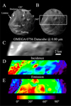 |
Fig. 1 (A) Latitude and longitude map of Phobos reoriented as the OMEGA 0756 datacube. The Stickney, Limtoc, and Reldresal craters are indicated with white arrows. (B) Area of Phobos observed by OMEGA. (C) Original OMEGA dataset at 0.80 μm (not yet Lommel-Seeliger corrected; see Section 3.2). (D) Incidence map. (E) Emission map produced through the use of the Phobos shape model (Willner et al. 2010) and the ancillary information of the spice kernels. |
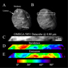 |
Fig. 2 (A) Latitude and longitude map of Phobos reoriented as the OMEGA 5851 datacube. The Stickney and Limtoc craters are indicated with white arrows. (B) Area of Phobos observed by OMEGA. (C) Original OMEGA dataset at 0.80 μm (not yet Lommel-Seeliger corrected; see Section 3.2). (D) Incidence map. (E) Emission map produced through the use of the Phobos shape model (Willner et al. 2010) and the ancillary information of the spice kernels. |
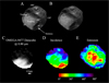 |
Fig. 3 (A) Latitude and longitude map of Phobos reoriented as the OMEGA 8477 datacube. (B) Area of Phobos observed by OMEGA. (C) Original OMEGA dataset at 0.80 μm (not yet Lommel-Seeliger corrected; see Section 3.2). (D) Incidence map. (E) Emission map produced through the use of the Phobos shape model (Willner et al. 2010) and the ancillary information of the spice kernels. |
3.2 Geometric and photometric correction
The three OMEGA datacubes (the non-photometrically corrected layer at 0.80 μm of each datacube is presented in Figs. 1–3C) were geometrically and photometrically corrected. In particular, the geometric correction was applied by using a self-written IDL code coupled with a NAIF IDL toolkit. The SPICE software is provided by the NASA JPL – Navigation and Ancillary information Facility (NAIF) and allows one to compute the relative position of the spectrometer and Phobos as well as the OMEGA pointing (Acton 1996; Acton et al. 2018). In order to identify the points of Phobos that are located in each detector pixel, we used the SINCPT procedure, exploiting a 3D model of the target produced by Willner et al. (2010). This 3D model is characterised by a 100 m/pixel spatial resolution, which is from one to nine times more resolved than the OMEGA dataset used. The illumination conditions, that is, the incidence (Figs. 1–3D) and emission (Figs. 1–3E), of each pixel present in the OMEGA cubes were obtained using the ILLUM NAIF procedure (see Acton (1996) for more detail) as shown in Stooke & Pajola (2019), Fig. 2, and in Fraeman et al. (2012), Fig. 1. We highlight that for the specific Fraeman et al. (2012) case, an inverted colour bar was used, when compared to ours. In addition, we did not limit the incidence angle representation of Figs. 1–3D to 85∘, as done by Fraeman et al. (2012). Rather, our chosen limit was 90∘. To get rid of the viewing geometry effects, we followed the same procedures as Pajola et al. (2018), where the Lommel-Seeliger disc function (LSDF) was applied to each pixel of the datacube. The LSDF is defined as

where i is the incidence angle and e is the emission angle. Both angles were computed starting from the incident and reflected light ray with respect to the normal of the Phobos facet. Each pixel I/F value was then divided by the corresponding disc function value. The term D (i,e) was derived from the radiative transfer theory, considering a single scattering particulate surface (Hapke 1981), and it turned out to be particularly suitable for D-type asteroids, Phobos (Pajola et al. 2018), and for very dark surfaces such as cometary nuclei (Fornasier et al. 2015) due to the predominance of the single scattering. In order to avoid limb effects, for all OMEGA cubes the pixels with an incidence angle larger than 80∘ were set to zero. The resulting disc-corrected RGB images are presented in Figs. 4A–C.
3.3 Spectral extraction
For each corrected OMEGA datacube, we selected some specific regions of interest (ROIs) identified visually on RGB images, where the R (0.90 μm), G (0.58 μm), and B (0.50 μm) channels were chosen to emphasise different colour units on the surface of the satellite (Figs. 4D–F). In particular, we focused our attention to the red and blue units located inside and nearby the Stickney crater (Basilevsky et al. 2014), when visible, and its closest surroundings. This was performed using the Esri-ENVI software. In order to maximise the signal-to-noise ratio of the I/F spectra obtained, we decided to consider ROIs with dimensions always larger than 50–70 pixels. Each obtained spectrum was normalised at 0.55 μm in order to allow relative I/F comparisons. The resulting spectra, associated standard deviations, and instrumental effects obtained for cube 0756 are presented in Fig. 5, while the ones of cube 5851 and the single spectrum of cube 8477 are presented in Fig. 6.
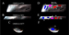 |
Fig. 4 (A–C) Disc-corrected RGB images (R is the 0.90 μm band, G is the 0.58 μm band, and B is the 0.50 μm band) of the three OMEGA cubes. (D–F) Regions of interest identified in the three RGB images. The ROI ID number is unique and is the same for each spectrum extracted (Figs. 5–6). |
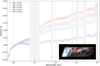 |
Fig. 5 Relative I/F spectra obtained for ROIs 1–5 extracted from the OMEGA 0756 cube. The error bars presented include both the associated standard deviations and the OMEGA instrumental uncertainties. The ID of the ROIs is the same as used in Figs. 4D–F. |
4 Results and discussion
4.1 Spectral properties and the possible 1 μm absorption band
Among all the considered OMEGA cubes, the 0756 dataset covers the largest portion of both the red and blue units of Phobos with the highest spatial scale. In particular, 0756 extends from the inner part of Stickney to the Limtoc crater to the Stickney north-eastern ejecta. Within this dataset, ROI1 is located fully inside the Stickney crater, ROI2 covers the blue unit at the easternmost side of the crater’s rim (this is the brightest area of Phobos, with an albedo that is 50 to 60% higher than Phobos average value, Fornasier et al. (2024)), and ROIs 3, 4, and 5 are at increasing distance from Stickney (Figs. 4A and D), with ROI4 located inside the Reldresal crater. The relative I/F spectra and associated standard deviations are presented in Fig. 5. As can be seen, the bluest and flattest spectrum is that of ROI2, as confirmed by its location in the slightly different HiRISE4 viewing angle (Basilevsky et al. 2014) and spatial scale image (blue box of Fig. 7). In contrast, the spectra derived from ROIs 3, 4 (within the 0756 cube, these two are the steepest in the NIR range), and 5 (this is the steepest in the Vis wavelength range) are steeper than the spectra extracted from the blue unit, as expected by the fact that they cover the red unit at different distance from Stickney’s rim.
The trends we describe confirm the Phobos surface’s distinction into red and blue units and show that there is not a sharp boundary between the two. Instead, as shown by the behaviour of the five ROIs, there appears to be a spectral transition from the blue unit towards the red one. For what concerns ROI1, it is already well known that the inner part of the Stickney crater does not show the bluest slope and colour (Fig. 7) since there appears to also be some patches belonging to the red unit (Basilevsky et al. 2014).
Among the spectra, there is an interesting feature identified from the ROI2 selection, namely, a possible absorption band at wavelengths ≥ 0.72 μm. This same absorption appears to also be present in ROIs 4 and 5. Before any possible interpretation is advanced, we cautiously highlight that the OMEGA VNIR and SWIR-C channels are affected by known bad bands between ∼0.9 and 1.1 μm (see Section 3.1). Moreover, these two OMEGA channels suffer from a decrease of sensitivity around their ∼1 μm wavelength boundary (Bibring et al. 2004). This means that the observed I/F decrease at wavelengths ≥ 0.70 μm, which is of the order of 2 (ROIs 4 and 5) to 7% (ROI2), can be entirely due to a decrease in the detectors’ sensitivity at the wavelength limit. Nevertheless, it is worth highlighting that such an I/F decrease is only present in the three mentioned ROI spectra, and it does not appear in any other of the observed and analysed ROIs despite the same VNIR and SWIR-C detectors being used. This said, the tentative absorption band would have a minimum in the ∼1.0 μm wavelength range, which is the typical position of the low calcium pyroxene 1 μm band and close to Fe/Mg olivine5; both are due to Fe2+ crystal field electronic transitions (Clark & Rencz 1999). This specific tentative absorption feature in the spectrum would highlight the presence of a basaltic compound on the surface of Phobos and support the absorption-like feature with a minimum close to 1.04 μm, which was obtained by Murchie et al. (1999) after re-analysing the ISM data.
When compared to the 0756 cube, the 5851 dataset is characterised by a better resolution (101 m versus 175 m). Despite covering a narrower area on Phobos (Fig. 2), it still shows the inner parts of Limtoc and Stickney, where we identified ROIs 6 and 7, respectively, and the proximal ejecta blanket, where our ROIs 8, 9, and 10 have been located (Fig. 4E). As is possible to see from Fig. 6, ROIs 6 and 7 are the least steep. This is consistent with the fact that are generally located inside the Stickney crater or close to its eastern rim. On the contrary, ROI8 presents the reddest slope in the full Vis-NIR despite its location in the blue unit. This can be explained by the fact that the area we selected is positioned over a particularly red crater and ejecta, as is clearly visible in Fig. 7. The I/F trend of ROI8 confirms, thanks to this highly resolved OMEGA cube, the presence of red patches located inside the blue ejecta of Stickney (Basilevsky et al. 2014); these patches were previously identified solely with the HiRISE camera. Moreover, the fact that there are red patches exhumed by younger craters that emplaced on Stickney ejecta supports the interpretation that the blue unit might be the fresh material coming from Stickney itself and that it is draped on top of the red older unit. As for 0756, the overall 5851 I/F spectra confirm, once again, that there is a spectral transition between the blue and red units, with a constantly increasing slope from the bluest to the reddest areas. The 8477 datacube (Fig. 6) has the noisiest I/F spectra among the whole dataset. This led us to consider only a single ROI, called ROI11, over the full dataset. The derived I/F spectrum lies in the middle of the NIR spectral trends observed from cube 5851, but it is one of the bluest in the Vis wavelength range. Such spectral behaviour is due to the locations of ROI11, which entirely covers the eastern ejecta of Stickney. In particular, this area is the blue unit presented in Fig. 7 with some red patches located in it but observed from the southern hemisphere of Phobos.
In order to relatively compare all OMEGA spectra obtained from the different ROIs, we decided to plot them together in Fig. 8. Here, a clear transition is visible from the bluest spectrum of ROI2 to the reddest one obtained from ROI8. We highlight that no previous datasets have shown such a wide range of spectral variation within the Phobos surface, and we point to the fact that besides the blue and red end-members, a smooth colour change is present on the Phobos sub-Mars hemisphere. Whether this is due to a slightly different mineralogical composition; different grain sizes and relative percentages of the surface components, as suggested by Pajola et al. (2018); or a phase reddening effect is not clear. (We highlight that there is a phase difference of 40∘ between OMEGA 0756 and 5851 cubes; see Table 1; and if similar to comet 67P, in the Vis range there would be a slope difference of 2 to 4%/100 nm, Fornasier et al. 2015.) Nevertheless, this smooth intermixed blanketing effect (i) is consistent with the interpretation of the blue unit as the ejecta produced by the impact that created Stickney and (ii) confirms the patchy aspect observed by Murchie & Erard (1996) and Murchie et al. (1999) and later confirmed by other authors (Murchie et al. 1999; Fraeman et al. 2014; Takir et al. 2022) for this area of Phobos (Basilevsky et al. 2014).
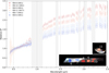 |
Fig. 6 Relative I/F spectra obtained from the ROIs 6–10 extracted from the OMEGA 5851 cube and from ROI 11 from the OMEGA 8477 cube. The error bars presented include both the associated standard deviations and the OMEGA instrumental uncertainties. The ID of the ROIs is the same as used in Figs. 4D–F. |
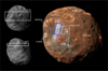 |
Fig. 7 Location of the OMEGA 0756 and 5851 cubes compared with the HiRISE 6.8 m spatial scale PSP_007769_9010_IRB image. The blue rectangle shows the location of ROI2, while the red rectangle shows the location of ROI8. |
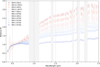 |
Fig. 8 Spectra extracted from all three analysed datacubes. All of these spectra have been normalised to 0.55 μm. One can clearly observe a gradual transition from the bluest spectrum (ROI2) to the reddest one (ROI8). The ID of the ROIs is the same as used for Figs. 4D–F and for Figs. 5 and 6. As in Figs. 5 and 6, the error bars presented include both the associated standard deviations and the OMEGA instrumental uncertainties. |
4.2 The Fe-, 1 μm band, and UV downturn distribution across the red and blue units of Phobos: The sub-Mars hemisphere case study
As studied by different authors (Pieters et al. 2000; Hapke 2001; Sasaki et al. 2001; Brunetto & Strazzulla 2005; Pieters & Noble 2016; DellaGiustina et al. 2020), SW can affect minor body surfaces in different ways depending on their mineralogical composition. Such effects include reddening or blueing of the continuum, rock vaporisation and melting, the formation of dark agglutinate glass, intense vitrification, and the creation of a nanoparticle phase rich in Fe-oxide. To better characterise the spatial distribution of both red and blue units of Phobos and to emphasise their mutual differences, we decided to derive a geographical distribution of the possible Fe-oxide presence on the surface of the Martian satellite. Indeed, if the blue unit is the result of ejecta deposition from the Stickney formation, then we would expect the red unit to be richer in products resulting from SW action since it is older than the blue ejecta and hence more weathered. In support of this, ROI2 (blue unit) photometric properties are different than the red unit, being the blue unit much brighter (Fornasier et al. 2024). Of all the considered OMEGA cubes, the 0756 dataset covers the largest portion of both the red and blue units of Phobos observed in the sub-Mars hemisphere and with the highest spatial scale (Fig. 9A). We therefore decided to focus entirely on this cube.
In order to trace the possible Fe-oxide on the dataset, we used the formula

where Rb is the I/F value at 0.71 μm, while Ra is the I/F value at 0.50 μm. This choice was taken since the Fe-oxide commonly reflects the Vis-red wavelength range (0.62–0.75 μm), while it absorbs the blue counterpart (≤0.5 μm, Clark & Rencz 1999). As can be seen from Fig. 9B, RFe is higher where the red unit is located, while it drastically drops over the blue unit. This trend is consistent with the fact that the red region might be richer in Fe-oxide than the blue unit and hence older, be much more affected by SW, and have a steeper visible spectrum. We nevertheless have to point out that recent works performed on the dark, carbonaceous B-type asteroid (101955) Bennu (DellaGiustina et al. 2020; Trang et al. 2021) have evidenced that its surface becomes bluer as it is affected by SW, which is exactly the opposite of what we are observing on Phobos. Since the real composition of the Martian satellite is not yet known and it might be spectrally similar to D- or T-type asteroids (e.g. Pajola et al. 2013 and discussion below), the effects of SW could be completely different despite the primitiveness of the objects considered (Lantz et al. 2015, 2017).
We then focused our attention to mapping the geographic distribution of the possible 1 μm absorption band. We used the band depth formula

where Rd is the I/F at λ = 0.87 μm, which is the minimum derivable from the OMEGA dataset, while Rc is the I/F at λ = 0.72 μm (i.e. the left shoulder discussed above). As can be seen from Fig. 9C, this I/F absorption only appears in the blue unit, confirming what we previously identified through ROI2. If confirmed by future datasets, this suggests that Stickney’s ejecta might be characterised by a basaltic compound coming from the subsurface layers of Phobos, which is not clearly distinguishable in the red unit of the satellite.
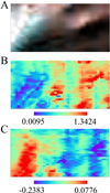 |
Fig. 9 (A) Cropped area of the OMEGA 0756 cube entirely focusing on the sub-Mars blue-red transition. (B) Obtained RFe values. (C) Obtained BD values. |
4.3 Comparison with mean asteroid classes and meteorites
The current literature suggests that Phobos Vis-NIR spectral behaviour resembles the dark and primitive objects (e.g. Pajola et al. 2013; Fraeman et al. 2014; Takir et al. 2022; Mason et al. 2023 and references herein), that is, D- and T-type asteroids, as well as possibly the C-type ones (see Section 2.0). In order to compare such classes with the obtained OMEGA I/F, we decided to select the spectra from ROIs 1, 2, 7, 8, and 10 because they well represent the full range of obtained spectral slopes from the steepest (ROI8) to the flattest (ROI2). As is possible to see from Fig. 10A, when we compare our ROIs with the Vis Bus & Binzel (2002a,b) mean asteroid types6 (normalised at 0.55 μm), we notice that no OMEGA ROI is similar to the C-type class, which is much flatter. However, the D- mean type appears to be much more similar in slope in the 0.45–0.8 μm range to our ROIs 8 and 10. The T-mean type is more akin to our ROI1 in the 0.45– 0.8 μm range. If we extend this comparison to the NIR spectral range using the Tholen (1984) asteroidal classes (Fig. 10B), we again see that the C-type class does not show any slope similarities with our ROIs’ spectra, even if we consider our bluest one (ROI2). This confirms the mismatch between the Phobos blue unit and the C-type mean classes (Murchie et al. 1999; Thomas et al. 1999). In contrast, the Tholen T-and D-types fall inside our ROIs 2 and 1, with the D-type appearing similar to the ROI1 slope. This general behaviour is confirmed when we compare the OMEGA spectra with different C-, D-, and T-type asteroids used as end-members, namely, (10) Hygea, (114) Kassandra and (570) Kythera, respectively (supplementary Fig. A.1). As mentioned in Yamamoto et al. (2018), we underline that various candidate spectra that can match the spectra of Phobos and Deimos since such trends have no undisputable diagnostic absorptions. Moreover, Yamamoto & Watanabe (2021) also reported that D-type spectra can be explained not only by carbonaceous chondritic objects but also by differentiated objects composed of rocky materials based on asteroidal taxonomic classes defined by the DeMeo & Carry (2014) model. This means that the Phobos similarity to D- and T-type spectra points to its surface primitiveness, but there are other spectrally explainable rocks, such as space-weathered anorthosite, that can represent its composition.
Our remaining ROIs (7, 8, and 10) are much steeper than the Tholen presented classes, and they have no match with the mean asteroidal types (although there might be some similarity in the Vis range with the extremely red Z-class of Mahlke et al. (2022), introduced for the Trojan asteroids and (269) Justitia). However, the observed Vis spectral slopes fall inside the TNOs and Centaurs BB and BR mean classes presented in Barucci et al. (2005); Perna et al. (2010), and Merlin et al. (2017), Supplementary Fig. A.2, at least at wavelengths less than 1.0 μm. Above this limit, the trend seems to decrease and becomes flatter, with the exception of the RR class, which comprises the reddest object in the Solar System. Nevertheless, an impact with a TNO is far from being advanced. Whether such trends are due to the SW effect steepening the already red spectra of Phobos or not is unclear, and it will need to be further investigated with future dedicated datasets.
The good match between some of the Phobos ROIs and D- and T-type asteroid spectra further support the general proposed spectral similarity between the Martian satellite and the dark carbon-rich (DeMeo & Carry 2014) primitive objects (Perna et al. 2018). For this reason, we decided to attempt a comparison between our spectra and some carbonaceous meteorites directly extracted from the RELAB spectral database (although we recall the different observing conditions, such as the phase angles mentioned above). The best results are given in Fig. 11
The Tagish Lake meteorite has been proposed as a possible analogue for D-type asteroids (Izawa et al. 2010; DeMeo et al. 2022), and it has already been used as a mixture component to fit different Phobos spectra (Pajola et al. 2013, 2018). Considering the different grain sizes of the samples, we found a good match for grain sizes of 0–25 μm and of 0–125 μm. These samples appear to show some slope similarity with ROI1, as visible in Fig. 11. They are therefore similar to the transitional unit between the red and the blue units.
The Kaidun meteorite, which is a CR2/CM2 carbonaceous chondrite, was already proposed as a possible Phobos analogue (Ivanov 2004). Pajola et al. (2012) attempted a comparison with Kaidun spectra, finding no match. Indeed, the spectra are particularly flatter and bluer with respect to the I/F derived from the red unit observed by Rosetta. However, since the presented OMEGA results show the bluest Phobos spectra obtained so far (much flatter than the blue unit spectra of Fraeman et al. 2012), the Kaidun meteorite now appears to likely match the ROI2 trend, that is, being the flattest representative of the blue unit we have in our dataset. Again, the best match involves very fine samples with grain sizes 0–45 μm.
The Cold Bokkeveld meteorite was considered by Fraeman et al. (2013) as a possible Phobos analogue due to the presence of cronstedtite, a low albedo mineral with a 0.6 μm absorption. It is a CM2 meteorite and also shows a flat trend in both the Vis and NIR wavelength range, comparable to the ROI2 spectrum. Nevertheless, it presents an absorption feature located at ∼0.75 μm, which is not present in the OMEGA blue unit.
The Murchison meteorite, a well-known carbonaceous chondrite, was identified by Fraeman et al. (2012) as a possible candidate for the interior of the Stickney crater and in the ejecta. Among all the Murchison spectra, which always show a 0.7 μm Fe2+ oxide electronic transition, the so-called Murchison fusion crust (Cloutis et al. 2018) is not characterised by this and shows an anhydrous aspect. In particular, it shows a shallow abruption-like feature at wavelengths slightly greater than 1 μm that seems to possibly reproduce the ROI2 OMEGA data. This could indicate that Phobos has undergone recrystallisation of the mineral, resulting in an anhydrous behaviour and explaining the absence of characteristic features in its spectrum.
As for the asteroid comparison, we did not find any match between the carbonaceous meteorites and the steep spectra of ROIs 7, 8, and 10. As mentioned before, this spectral behaviour can be due to SW or some other heavy processes on the surface. This very peculiar aspect of the Phobos spectrum needs to be further investigated with future dedicated datasets.
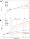 |
Fig. 10 (A) Comparison between the ROI spectra selected and the Vis Bus & Binzel (2002a,b) D-, T- and C-mean types normalised at 0.55 μm. (B) Comparison between the ROI spectra selected and the Vis-NIR Tholen (1984) D-, T- and C-mean types normalised at 0.55 μm. |
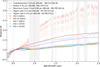 |
Fig. 11 Comparison between the selected ROI spectra and the Cold Bokkeveld, Kaidun, Murchison, and Tagish Lake meteorites. |
5 Conclusions
We have analysed three different Mars Express/OMEGA Phobos datacubes (0756, 5851, 8477) in the wavelength range 0.4–2.5 μm, correcting them both geometrically and photometrically. Through this dataset, we have studied the spectral behaviour of both the red and blue units of the Martian satellite. In particular, we not only focused on the Stickney crater and its closest surroundings but also on the Limtoc and Reldresal craters. After extracting the OMEGA spectra of 11 different ROIs, our data spanned from an almost flat spectrum belonging to the bluest Stickney ejecta (ROI2) to a steep red spectrum extracted from a particularly red unnamed crater emplaced in the blue unit of the Phobos sub-Mars hemisphere (ROI8); the crater was previously discovered by the MRO/HiRISE camera. Between these two end-members, we identified a wide range of spectral slope variation within the Phobos surface never observed before. This suggests that besides the blue and red end-members, a smooth colour change is present on the satellite sub-Mars hemisphere. Such a smooth intermixed blanketing effect is consistent with the interpretation of the blue unit being the ejecta produced by the impact that created Stickney and confirms the blue and red intermixed aspect discovered by Murchie & Erard (1996). Within the bluest spectrum obtained, we tentatively identified an absorption band (2–7%) located in the 0.7–1.3 μm spectral range. Such a feature could be due to the presence of Fe2+ electronic transitions indicating the presence of olivine (the 1.0 μm absorption), hence suggesting a basaltic component on Phobos. However, one main problem must be noted with this interpretation: The real minimum of the band is not visible due to the boundary of the OMEGA VNIR and SWIR-C detectors. Therefore, the observed I/F decrease can also be due to a decrease in the detector sensitivity at the wavelength limit. Nevertheless, it is worth highlighting that this possible absorption is only present in the ROI2, 4, and 5 spectra, while it does not appear in any other observed ROIs of all OMEGA datasets, despite the same VNIR and SWIR-C detectors being used. By comparing the Phobos Vis-NIR extracted spectra with asteroid mean types, we confirmed the similarity between Phobos spectra and primitive D-/T-type objects. However, the reddest obtained spectra largely exceed even the D-type spectral slopes but may be compatible with the reddest Z-type class recently introduced by Mahlke et al. (2022). Whether this trend is the result of SW or not is still under discussion, but with the current dataset, we cannot solve this conundrum. By comparing the OMEGA Phobos results with multiple carbonaceous meteorites, the bluest spectra show similar trends to the Cold Bokkeveld, Kaidun and Murchison fusion crust, although some differences clearly appear in the 0.6–0.8 μm range, especially with the Cold Bokkeveld meteorite. In contrast, the Tagish Lake meteorite Vis-NIR trends are more similar to some transitional (ROI1) OMEGA spectra. Nevertheless, as for the asteroid comparison, we find no match between the reddest Phobos spectra (ROI10 and ROI8) and primitive or dark meteorite samples.
The results are particularly useful in light of the forthcoming observations of Phobos by the MMX InfraRed Spectrometer Barucci et al. (MIRS; 2021) on board the JAXA/Martian Moons eXploration probe (Kuramoto et al. 2022). Indeed, the ROIs we have identified will be observed by MIRS with both a much better spatial scale and spectral resolution, hence leading to a better understanding of the satellite’s mineralogical composition and its controversial origin.
Acknowledgements
This work is dedicated to the memory of Dr. Brigitte Gondet. We would like to thank the anonymous Referee for the important and constructive comments received. This research utilises spectra acquired with the NASA RELAB facility at Brown University. G.P., S.F. and M.A.B. acknowledges the support of the Centre National d’Études Spatiales (CNES). J.R.B. and G.P. acknowledge support from Agenzia Spaziale Italiana (ASI) with grant ASI-INAF agreement 2022-1-HH.0.
Appendix A Additional figures
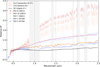 |
Fig. A.1 Comparison between the selected ROI spectra and the spectra normalised at 0.55 μm of asteroids (114) Kassandra (D-/T-type), (570) Kythera (D-type), and (10) Hygea (C-type). |
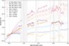 |
Fig. A.2 Comparison between the selected ROI spectra and the spectra normalised at 0.55 μm of RR, IR, BR, and BB TNO mean classes of Barucci et al. (2005); Perna et al. (2010); Merlin et al. (2017). |
References
- Acton, C. H., 1996, Planet. Space Sci., 44, 65 [Google Scholar]
- Acton, C., Bachman, N., Semenov, B., & Wright, E., 2018, Planet. Space Sci., 150, 9 [Google Scholar]
- Andert, T. P., Rosenblatt, P., Pätzold, M., et al. 2010, Geophys. Res. Lett., 37, L09202 [Google Scholar]
- Bagheri, A., Khan, A., Efroimsky, M., Kruglyakov, M., & Giardini, D., 2021, AAS/Div. Planet. Sci. Meeting Abstracts, 53, 201.03 [Google Scholar]
- Barucci, M. A., Belskaya, I. N., Fulchignoni, M., & Birlan, M., 2005, AJ, 130, 1291 [CrossRef] [Google Scholar]
- Barucci, M. A., Reess, J.-M., Bernardi, P., et al. 2021, Earth, Planets and Space, 73, 211 [NASA ADS] [CrossRef] [Google Scholar]
- Basilevsky, A. T., Lorenz, C. A., Shingareva, T. V., et al. 2014, Planet. Space Sci., 102, 95 [CrossRef] [Google Scholar]
- Bertaux, J. L., Montmessin, F., Gondet, B., et al. 2016, Ann. Lunar Planet. Sci. Conf., 47, 2177 [Google Scholar]
- Bibring, J. P., Soufflot, A., Berthé, M., et al. 2004, ESA SP, 1240, 37 [Google Scholar]
- Brunetto, R., & Strazzulla, G., 2005, Icarus, 179, 265 [NASA ADS] [CrossRef] [Google Scholar]
- Bus, S. J., & Binzel, R. P. 2002a, Icarus, 158, 146 [Google Scholar]
- Bus, S. J., & Binzel, R. P. 2002b, Icarus, 158, 106 [CrossRef] [Google Scholar]
- Cantor, B. A., Wolff, M. J., Thomas, P. C., James, P. B., & Jensen, G., 1999, Icarus, 142, 414 [NASA ADS] [CrossRef] [Google Scholar]
- Christensen, P. R., Anderson, D. L., Chase, S. C., et al. 1992, J. Geophys. Res., 97, 7719 [Google Scholar]
- Clark, R. N., & Rencz, A., 1999, Spectroscopy of Rocks and Minerals, and Principles of Spectroscopy (Hoboken: John Wiley and Sons), 11, 3 [Google Scholar]
- Cloutis, E. A., Pietrasz, V. B., Kiddell, C., et al. 2018, Icarus, 305, 203 [NASA ADS] [CrossRef] [Google Scholar]
- Craddock, R. A., 2011, Icarus, 211, 1150 [NASA ADS] [CrossRef] [Google Scholar]
- DellaGiustina, D. N., Burke, K. N., Walsh, K. J., et al. 2020, Science, 370, eabc3660 [Google Scholar]
- DeMeo, F. E., & Carry, B., 2014, Nature, 505, 629 [NASA ADS] [CrossRef] [Google Scholar]
- DeMeo, F. E., Burt, B. J., Marsset, M., et al. 2022, Icarus, 380, 114971 [NASA ADS] [CrossRef] [Google Scholar]
- Formisano, V., Angrilli, F., Arnold, G., et al. 2005, Planet. Space Sci., 53, 963 [Google Scholar]
- Fornasier, S., Hasselmann, P. H., Barucci, M. A., et al. 2015, A&A, 583, A30 [NASA ADS] [CrossRef] [EDP Sciences] [Google Scholar]
- Fornasier, S., Wargnier, A., Hasselmann, P. H., et al. 2024, A&A, 686, A203 [NASA ADS] [CrossRef] [EDP Sciences] [Google Scholar]
- Fraeman, A. A., Arvidson, R. E., Murchie, S. L., et al. 2012, J. Geophys. Res. Planets, 117, E00J15 [Google Scholar]
- Fraeman, A. A., Murchie, S. L., Arvidson, R. E., Rivkin, A. S., & Morris, R. V., 2013, Ann. Lunar Planet. Sci. Conf., 44, 1572 [Google Scholar]
- Fraeman, A. A., Murchie, S. L., Arvidson, R. E., et al. 2014, Icarus, 229, 196 [NASA ADS] [CrossRef] [Google Scholar]
- Giuranna, M., Roush, T. L., Duxbury, T., et al. 2011, Planet. Space Sci., 59, 1308 [NASA ADS] [CrossRef] [Google Scholar]
- Glotch, T. D., Edwards, C. S., Yesiltas, M., et al. 2018, J. Geophys. Res. Planets, 123, 2467 [Google Scholar]
- Grundy, W. M., & Fink, U., 1991, LPI Contrib., 765, 77 [Google Scholar]
- Hapke, B., 1981, J. Geophys. Res., 86, 4571 [NASA ADS] [Google Scholar]
- Hapke, B., 2001, J. Geophys. Res., 106, 10039 [NASA ADS] [CrossRef] [Google Scholar]
- Hyodo, R., Genda, H., Charnoz, S., & Rosenblatt, P., 2017, ApJ, 845, 125 [NASA ADS] [CrossRef] [Google Scholar]
- Ivanov, A. V., 2004, Solar Syst. Res., 38, 97 [Google Scholar]
- Izawa, M. R., Flemming, R. L., King, P. L., Peterson, R. C., & McCausland, P. J., 2010, Meteor. Planet. Sci., 45, 675 [Google Scholar]
- Jacobson, R. A., & Lainey, V., 2014, Planet. Space Sci., 102, 35 [CrossRef] [Google Scholar]
- Kuramoto, K., Kawakatsu, Y., Fujimoto, M., et al. 2022, Earth Planet. Space, 74, 12 [Google Scholar]
- Lantz, C., Brunetto, R., Barucci, M. A., et al. 2015, A&A, 577, A41 [NASA ADS] [CrossRef] [EDP Sciences] [Google Scholar]
- Lantz, C., Brunetto, R., Barucci, M. A., et al. 2017, Icarus, 285, 43 [CrossRef] [Google Scholar]
- Lucey, P. G., Bell, J. F., & Piscitelli, J. R., 1989, Lunar Planet. Sci. Conf., 20, 598 [Google Scholar]
- Lynch, D. K., Russell, R. W., Rudy, R. J., et al. 2007, AJ, 134, 1459 [Google Scholar]
- Mahlke, M., Carry, B., & Mattei, P. A., 2022, A&A, 665, A26 [NASA ADS] [CrossRef] [EDP Sciences] [Google Scholar]
- Mason, J. P., Patel, M. R., Pajola, M., et al. 2023, J. Geophys. Res. Planets, 128, e2023JE008002 [Google Scholar]
- Merlin, F., Hromakina, T., Perna, D., Hong, M. J., & Alvarez-Candal, A., 2017, A&A, 604, A86 [NASA ADS] [CrossRef] [EDP Sciences] [Google Scholar]
- Murchie, S., & Erard, S., 1996, Icarus, 123, 63 [CrossRef] [Google Scholar]
- Murchie, S. L., Britt, D. T., Head, J. W., et al. 1991, J. Geophys. Res. Solid Earth, 96, 5925 [Google Scholar]
- Murchie, S., Thomas, N., Britt, D., Herkenhoff, K., & Bell III, J. F. 1999, J. Geophys. Res. Planets, 104, 9069 [Google Scholar]
- Murchie, S., Arvidson, R., Bedini, P., et al. 2007, J. Geophys. Res. Planets, 112, E05S03 [Google Scholar]
- Murchie, S. L., Choo, T., Humm, D., et al. 2008, Ann. Lunar Planet. Sci. Conf., 39, 1434 [Google Scholar]
- Pajola, M., Lazzarin, M., Bertini, I., et al. 2012, MNRAS, 427, 3230 [NASA ADS] [CrossRef] [Google Scholar]
- Pajola, M., Lazzarin, M., Dalle Ore, C. M., et al. 2013, ApJ, 777, 127 [NASA ADS] [CrossRef] [Google Scholar]
- Pajola, M., Roush, T., Dalle Ore, C., Marzo, G. A., & Simioni, E., 2018, Planet. Space Sci., 154, 63 [NASA ADS] [CrossRef] [Google Scholar]
- Pang, K. D., Rhoads, J. W., Lane, A. L., & Ajello, J. M., 1980, Nature, 283, 277 [Google Scholar]
- Pascu, D., Erard, S., Thuillot, W., & Lainey, V., 2014, Planet. Space Sci., 102, 2 [Google Scholar]
- Perna, D., Barucci, M. A., Fornasier, S., et al. 2010, A&A, 510, A53 [NASA ADS] [CrossRef] [EDP Sciences] [Google Scholar]
- Perna, D., Barucci, M. A., Fulchignoni, M., et al. 2018, Planet. Space Sci., 157, 82 [CrossRef] [Google Scholar]
- Perrier, S., Stern, A. S., & Bertaux, J. L., 2004, AAS/Div. Planet. Sci. Meeting Abstracts, 36, 31.09 [Google Scholar]
- Pieters, C. M., & Noble, S. K., 2016, J. Geophys. Res. Planets, 121, 1865 [CrossRef] [Google Scholar]
- Pieters, C. M., Taylor, L. A., Noble, S. K., et al. 2000, Meteor. Planet. Sci., 35, 1101 [NASA ADS] [CrossRef] [Google Scholar]
- Poggiali, G., Matsuoka, M., Barucci, M. A., et al. 2022, MNRAS, 516, 465 [NASA ADS] [CrossRef] [Google Scholar]
- Rivkin, A. S., Brown, R. H., Trilling, D. E., Bell, J. F., & Plassmann, J. H., 2002, Icarus, 156, 64 [NASA ADS] [CrossRef] [Google Scholar]
- Ronnet, T., Vernazza, P., Mousis, O., et al. 2016, ApJ, 828, 109 [Google Scholar]
- Rosenblatt, P., 2011, A&A Rev., 19, 44 [NASA ADS] [CrossRef] [Google Scholar]
- Rosenblatt, P., & Charnoz, S., 2012, Icarus, 221, 806 [NASA ADS] [CrossRef] [Google Scholar]
- Sasaki, S., Nakamura, K., Hamabe, Y., Kurahashi, E., & Hiroi, T., 2001, Nature, 410, 555 [NASA ADS] [CrossRef] [Google Scholar]
- Stooke, P., & Pajola, M., 2019, Mapping Irregular Bodies, ed. H. Hargitai (Cham: Springer International Publishing), 191 [Google Scholar]
- Takir, D., Matsuoka, M., Waiters, A., Kaluna, H., & Usui, T., 2022, Icarus, 371, 114691 [NASA ADS] [CrossRef] [Google Scholar]
- Tholen, D. J., 1984, PhD thesis, University of Arizona, USA [Google Scholar]
- Tholen, D. J., & Barucci, M. A., 1989, in Asteroids II, eds. R. P. Binzel, T. Gehrels, & M. S. Matthews (Tucson: University of Arizona Press), 298 [Google Scholar]
- Thomas, N., Britt, D. T., Herkenhoff, K. E., et al. 1999, J. Geophys. Res., 104, 9055 [NASA ADS] [CrossRef] [Google Scholar]
- Trang, D., Thompson, M. S., Clark, B. E., et al. 2021, Planet. Sci. J., 2, 68 [Google Scholar]
- Tsiganis, K., Gomes, R., Morbidelli, A., & Levison, H. F., 2005, Nature, 435, 459 [Google Scholar]
- Walsh, K. J., Morbidelli, A., Raymond, S. N., O’Brien, D. P., & Mandell, A. M., 2011, Nature, 475, 206 [Google Scholar]
- Willner, K., Oberst, J., Hussmann, H., et al. 2010, Earth Planet. Sci. Lett., 294, 541 [Google Scholar]
- Witasse, O., Duxbury, T., Chicarro, A., et al. 2014, Planet. Space Sci., 102, 18 [Google Scholar]
- Yamamoto, S., & Watanabe, S.-i., 2021, J. Geophys. Res. Planets, 126, e06669 [Google Scholar]
- Yamamoto, S., Watanabe, S., & Matsunaga, T., 2018, Geophys. Res. Lett., 45, 1305 [Google Scholar]
The Murchie & Erard (1996) colour index is defined as the ratio between the Vis (0.5 μm) and NIR(0.95 μm) bands.
ESA PSA Node: https://archives.esac.esa.int/psa/ftp/MARS-EXPRESS/OMEGA/
All distances presented here are computed from the MEX spacecraft to the Phobos surface.
This image is publicly available at https://www.uahirise.org/releases/phobos/
The 1 μm band absorption of olivine is caused by crystal field absorption with splitting the energy levels of d-orbital electrons of Fe2+.
We here highlight that the considered OMEGA observations have been obtained at phase angles of 63∘, 70∘ and 101∘ (Table 1), i.e. much larger than those obtained for mean asteroid types (<25∘), as well as meteorites. Such comparison should be then taken carefully since phase reddening on Phobos could be important, as observed for comet 67P (Fornasier et al. 2015). However, we point out that the Phobos reddest spectra obtained are particularly similar to the mean D-type (Perna et al. 2018).
All Tables
All Figures
|
Fig. 1 (A) Latitude and longitude map of Phobos reoriented as the OMEGA 0756 datacube. The Stickney, Limtoc, and Reldresal craters are indicated with white arrows. (B) Area of Phobos observed by OMEGA. (C) Original OMEGA dataset at 0.80 μm (not yet Lommel-Seeliger corrected; see Section 3.2). (D) Incidence map. (E) Emission map produced through the use of the Phobos shape model (Willner et al. 2010) and the ancillary information of the spice kernels. |
| In the text | |
|
Fig. 2 (A) Latitude and longitude map of Phobos reoriented as the OMEGA 5851 datacube. The Stickney and Limtoc craters are indicated with white arrows. (B) Area of Phobos observed by OMEGA. (C) Original OMEGA dataset at 0.80 μm (not yet Lommel-Seeliger corrected; see Section 3.2). (D) Incidence map. (E) Emission map produced through the use of the Phobos shape model (Willner et al. 2010) and the ancillary information of the spice kernels. |
| In the text | |
|
Fig. 3 (A) Latitude and longitude map of Phobos reoriented as the OMEGA 8477 datacube. (B) Area of Phobos observed by OMEGA. (C) Original OMEGA dataset at 0.80 μm (not yet Lommel-Seeliger corrected; see Section 3.2). (D) Incidence map. (E) Emission map produced through the use of the Phobos shape model (Willner et al. 2010) and the ancillary information of the spice kernels. |
| In the text | |
|
Fig. 4 (A–C) Disc-corrected RGB images (R is the 0.90 μm band, G is the 0.58 μm band, and B is the 0.50 μm band) of the three OMEGA cubes. (D–F) Regions of interest identified in the three RGB images. The ROI ID number is unique and is the same for each spectrum extracted (Figs. 5–6). |
| In the text | |
|
Fig. 5 Relative I/F spectra obtained for ROIs 1–5 extracted from the OMEGA 0756 cube. The error bars presented include both the associated standard deviations and the OMEGA instrumental uncertainties. The ID of the ROIs is the same as used in Figs. 4D–F. |
| In the text | |
|
Fig. 6 Relative I/F spectra obtained from the ROIs 6–10 extracted from the OMEGA 5851 cube and from ROI 11 from the OMEGA 8477 cube. The error bars presented include both the associated standard deviations and the OMEGA instrumental uncertainties. The ID of the ROIs is the same as used in Figs. 4D–F. |
| In the text | |
|
Fig. 7 Location of the OMEGA 0756 and 5851 cubes compared with the HiRISE 6.8 m spatial scale PSP_007769_9010_IRB image. The blue rectangle shows the location of ROI2, while the red rectangle shows the location of ROI8. |
| In the text | |
|
Fig. 8 Spectra extracted from all three analysed datacubes. All of these spectra have been normalised to 0.55 μm. One can clearly observe a gradual transition from the bluest spectrum (ROI2) to the reddest one (ROI8). The ID of the ROIs is the same as used for Figs. 4D–F and for Figs. 5 and 6. As in Figs. 5 and 6, the error bars presented include both the associated standard deviations and the OMEGA instrumental uncertainties. |
| In the text | |
|
Fig. 9 (A) Cropped area of the OMEGA 0756 cube entirely focusing on the sub-Mars blue-red transition. (B) Obtained RFe values. (C) Obtained BD values. |
| In the text | |
|
Fig. 10 (A) Comparison between the ROI spectra selected and the Vis Bus & Binzel (2002a,b) D-, T- and C-mean types normalised at 0.55 μm. (B) Comparison between the ROI spectra selected and the Vis-NIR Tholen (1984) D-, T- and C-mean types normalised at 0.55 μm. |
| In the text | |
|
Fig. 11 Comparison between the selected ROI spectra and the Cold Bokkeveld, Kaidun, Murchison, and Tagish Lake meteorites. |
| In the text | |
|
Fig. A.1 Comparison between the selected ROI spectra and the spectra normalised at 0.55 μm of asteroids (114) Kassandra (D-/T-type), (570) Kythera (D-type), and (10) Hygea (C-type). |
| In the text | |
|
Fig. A.2 Comparison between the selected ROI spectra and the spectra normalised at 0.55 μm of RR, IR, BR, and BB TNO mean classes of Barucci et al. (2005); Perna et al. (2010); Merlin et al. (2017). |
| In the text | |
Current usage metrics show cumulative count of Article Views (full-text article views including HTML views, PDF and ePub downloads, according to the available data) and Abstracts Views on Vision4Press platform.
Data correspond to usage on the plateform after 2015. The current usage metrics is available 48-96 hours after online publication and is updated daily on week days.
Initial download of the metrics may take a while.