| Issue |
A&A
Volume 697, May 2025
|
|
|---|---|---|
| Article Number | A50 | |
| Number of page(s) | 22 | |
| Section | Numerical methods and codes | |
| DOI | https://doi.org/10.1051/0004-6361/202453647 | |
| Published online | 12 May 2025 | |
The EXOD search for faint transients in XMM-Newton observations
Part II
1
Institute for Research in Astrophysics and Planetology (IRAP), CNRS,
31400
Toulouse,
France
2
European Space Agency (ESA), European Space Astronomy Centre (ESAC),
Camino Bajo del Castillo s/n,
28692
Villanueva de la Cañada, Madrid,
Spain
3
Astronomical Institute, Academy of Sciences,
Boční II 1401,
14131
Prague,
Czech Republic
4
Jodrell Bank Centre for Astrophysics, University of Manchester,
Oxford Road,
Manchester
M13 9PL,
UK
5
Telespazio France, Space Systems and Operations (SSO),
31110
Toulouse,
France
6
Leibniz-Institut für Astrophysik Potsdam (AIP),
An der Sternwarte 16,
14482
Potsdam,
Germany
7
Université de Strasbourg, CNRS, Observatoire astronomique de Strasbourg, UMR 7550,
67000
Strasbourg,
France
* Corresponding author.
Received:
31
December
2024
Accepted:
12
March
2025
Abstract
Context. The XMM-Newton observatory has accumulated a vast archive of over 17 000 X-ray observations over the last 25 years. However, the standard data processing pipelines may fail to detect certain types of transient X-ray sources, due to their short-lived or dim nature. Identifying these transient sources is important for understanding the full range of temporal X-ray behaviour, as well as understanding the types of sources that could be routinely detected by future missions such as Athena.
Aims. The aim of this work is to reprocess XMM-Newton archival observations using newly developed dedicated software in order to identify neglected and missed transient X-ray sources that were not detected by the existing pipeline.
Methods. We used a new approach that builds upon previous methodologies, by transforming event lists into data cubes, which are then searched for transient variability in short time windows. Our method enhances the detection capabilities in the Poisson regime by accounting for the statistical properties of sparse count rates, and allowing the search for transients in previously discarded periods of high background activity.
Results. Our reprocessing efforts identified 32 247 variable sources at the three-sigma level and 4083 sources at the five-sigma level in 12 926 XMM archival observations. We highlight four noteworthy sources: a candidate quasi-periodic eruption (QPE), a new magnetar candidate, a previously undetected Galactic hard X-ray burst, and a possible X-ray counterpart to a Galactic radio pulsar.
Conclusions. Our method demonstrates a new, fast, and effective way to process event list data from XMM-Newton, which is efficient in finding rapid outburst-like or eclipsing behaviour. This technique can be adapted for use with future telescopes, such as Athena, and can be generalised to other photon counting instruments operating in the low-count Poisson regime.
Key words: instrumentation: detectors / techniques: image processing / X-rays: general
© The Authors 2025
 Open Access article, published by EDP Sciences, under the terms of the Creative Commons Attribution License (https://creativecommons.org/licenses/by/4.0), which permits unrestricted use, distribution, and reproduction in any medium, provided the original work is properly cited.
This article is published in open access under the Subscribe to Open model. This email address is being protected from spambots. You need JavaScript enabled to view it. to support open access publication.
1 Introduction
Since its launch in December 1999, XMM-Newton (Jansen et al. 2001) has been detecting X-ray photons in the 0.2–12.0 keV energy range using the European Photon Imaging Camera (EPIC). The most recent XMM serendipitous source catalogue (Webb et al. 2020), 4XMM-DR14, contains 13 864 archival observations, and 1 035 832 detections of which 21 570 (∼2%) are flagged to be intra-observation variable. Since many sources have been detected more than once, these one million detections correspond to 692 109 unique sources, of which 6311 (~ 0.9%) are flagged as variable; this lower percentage is due to selection bias, as variable sources often have multiple observations.
The XMM pipeline detection routine first combines all the photons detected on each of the three instruments that compose the EPIC (pn, MOS1, and MOS2) instrument to create an image; standardised detection algorithms are then applied to this image to detect sources (see Masias et al. 2012, for a review on source detection methods). Sources with more than 100 EPIC counts are then further analysed for transient behaviour using two methods: (1) a χ2 test comparing time series of the detection to a null hypothesis of a constant count rate, (Watson et al. 2009) and (2) a measure of the fractional variability amplitude Fvar (Rosen et al. 2016).
The χ2 statistic is suitable for binned data where the distribution of events in each time bin can be assumed to be Gaussian; it is not suitable for counts below ~10–20 per bin (see Cash 1979). This is in part why the requirement of at least 100 total counts for the variability analysis is specified. This prescription results in approximately two-thirds of all detections (663 519 out of 1 035 832) not being analysed for transient behaviour. The standard pipeline variability analysis is well suited for characterising the variability in detections with abundant counts and gradual variations, but is less suited to sources that are photon limited and show sharp spikes or dips in their time series.
The awareness that short-term X-ray transients are lying undiscovered within the XMM archive has motivated several studies to bring them to light. To date, three major studies have systematically searched the entire XMM catalogue, EXTraS (De Luca et al. 2016, 2021), a search for supernovae shock breakout (Alp & Larsson 2020), and the first version of the algorithm presented in this paper (Pastor-Marazuela et al. 2020). It is also worth mentioning the STATiX pipeline (Ruiz et al. 2024) that is specifically designed for the detection of transients in XMM data has not yet been applied to the data archive.
The method presented in this paper is a development of the method presented in Pastor-Marazuela et al. (2020), but has been entirely re-written ‘from the ground up’, as part of the XMM2Athena project (Webb et al. 2023). We have made numerous changes to the way that transients are identified, and importantly have incorporated changes that allow us to probe the previously excluded time periods with background flaring caused by soft proton flares, which accounts for around 15% of all observing exposure.
X-ray transients have a variety of origins, and when conducting broad searches, it is essential to consider all potential mechanisms. In this section we discuss some possible underlying causes of these transients, along with their characteristic timescales and 0.2–12.0 keV X-ray luminosities.
Stellar flares: Magnetic reconnection in the atmospheres of stars can result in sudden bursts of energy, which can be detected across the electromagnetic spectrum (e.g. Kowalski 2024). Flares from cool stars (spectral type F-M) as well as young stellar objects (YSOs) are known to be particularly abundant in the X-ray bands. Stellar flares have timescales of around 104–105 seconds and have peak luminosities of ~1029–1032 erg s−1. (e.g. Imanishi et al. 2003; Pye et al. 2015)
X-ray binaries (XRBs): X-ray binaries, both high-mass and low-mass (HMXBs & LMXBs), release X-rays as material is accreted onto a compact object, either a neutron star (NS) or a black hole (BH). These sources are known to be variable on a wide range of timescales from seconds to months, and have luminosities in the range ~1035–1039 erg s−1 (e.g. Lewin & van der Klis 2006; Fabbiano 2006).
Cataclysmic variables (CVs): closely interacting binaries involving accretion onto a white dwarf are powerful sources of X-rays (see Warner 1995; Kuulkers et al. 2010). CVs are often subclassified depending on the magnetic field strength of the white dwarf. Non-magnetic CVs (sometimes called dwarf novae) have accretion discs extending down to the compact object and are known to display large, often repeating outbursts over a few days before returning to quiescence. Magnetic CVs are sometimes referred to as (intermediate) polars and may have truncated accretion discs where X-rays can be emitted by a standing shock above the magnetic poles of the WD (e.g. Aizu 1973; Page & Shaw 2022). CVs span the luminosity range ~1029–1035 erg s−1 (see Suleimanov et al. 2022; Schwope et al. 2024). Additionally, these sources usually have orbital periods of the order of hundreds of minutes, which can be evident in the light curves of eclipsing sources (e.g. Schwope et al. 2001). A rare phenomenon manifesting as a soft X-ray flash with a luminosity of ~1038 erg s−1 has recently been observed in YZ Ret (König et al. 2022). This fireball phase is explained as the rapid expansion of the surrounding envelope of the WD, following the runaway thermonuclear burning on its surface and is predicted to last several hours (see Kato et al. 2015).
Type I and II X-ray bursts: Type I X-ray bursts are caused by runaway thermonuclear explosions on the surface of NSs. These bursts have been detected in over 121 sources (e.g. Galloway et al. 2020; Galloway & Keek 2021). The bursts have a characteristic profile of a fast rise (≤ 1–10 s) followed by an exponential decay (~ 10–100 s). Type I X-ray bursts peak luminosities cluster around ~ 1038 erg s−1, which has motivated their possible use as standard candles (see Kuulkers et al. 2003). Type II bursts are known to exist in only two sources and are seen to repeat of the order of ~ 10–20 s. Although they have been known for over 45 years, their nature still remains unclear (e.g. Bagnoli et al. 2015).
Magnetars (AXP, SGRs & LGRs): Magnetars (Duncan & Thompson 1992), are young neutron stars with magnetic fields exceeding approximately ⪺1013 G. They are known under a variety of different aliases such as anomalous X-ray pulsars (AXPs), soft and long gamma repeaters (SGRs & LGRs) (e.g. Turolla et al. 2015). Magnetars exhibit a wide range of variability: short bursts (lasting <100 ms with L ~ 1036–1043 erg s−1), outbursts (rise times of the order of ~10–100s and reaching ~1036 erg s−1), and giant flares (seconds to minutes with L ~ 1044–1047 erg s−1) (see Kaspi & Beloborodov 2017). Pulse periods have been identified for 26 magnetars (see Olausen & Kaspi 2014) and average around a few seconds, while their quiescent X-ray luminosities lie in the range of ~1032–1035 erg s−1.
Gamma-ray bursts (GRBs): As their name suggests, the emission from GRBs primarily peak at higher energies; however, their afterglow emission can be detected in X-rays and lower energy bands. Lasting from seconds to hours, GRBs are typically divided into short and long, and are thought to arise respectively from the mergers of neutron stars and from the collapse of massive stars (e.g. Kumar & Zhang 2015). The observed X-ray luminosities for GRB afterglows decrease over time, but typically range from ~1043–1049 erg s−1 over a period of 5 minutes to 24 hours (see D’Avanzo et al. 2012). GRBs can also be related to gravitational wave events. For example, the detection of a transient X-ray counterpart to the NS-NS merger GW 170817 is suspected to be the afterglow from an off-axis GRB (see Troja et al. 2017).
Tidal disruption events (TDEs): Stars in galactic nuclei can be captured or tidally disrupted by the supermassive black hole (e.g. Rees 1988). This process can result in luminous X-ray flares (~ 1044 erg s−1) that may last months to years (e.g. Saxton et al. 2021). A theoretical subclass of TDEs involves the tidal disruption of a white dwarf by an intermediate-mass black hole (IMBH) (e.g. Maguire et al. 2020); these would have considerably shorter evolution timescales than regular TDEs with the rise times possibly occurring on timescales of hundred of seconds as opposed to days (e.g Jonker et al. 2013).
Quasi-periodic eruptions (QPEs): Recently discovered large amplitude (peaking at L ~ 1042–1043 erg s−1) soft QPEs from several galactic nuclei (See: Miniutti et al. 2019; Giustini et al. 2020; Arcodia et al. 2021; Chakraborty et al. 2021; Arcodia et al. 2022; Miniutti et al. 2023; Quintin et al. 2023; Webbe & Young 2023; Arcodia et al. 2024) have resulted in several suggestions for their origin, including repeated partial TDEs of stars by a SMBH, or interactions between stars and SMBH accretion discs (e.g. Linial & Quataert 2024). Recent discoveries in one source would appear to strongly link QPEs and TDEs (e.g. Quintin et al. 2023; Nicholl et al. 2024). The timescales of the outbursts and their recurrence are around a few hours in the X-ray; however, some galactic nuclei have been seen with longer recurrence times (days to years) and are sometimes classified as repeating nuclear transients (e.g. Guolo et al. 2024).
Supernovae shock breakouts (SBOs): SBOs occur when the shock wave from a supernova breaks through the outer layers of the star. This process can produce a bright X-ray/UV flash on timescales of seconds to fractions of an hour; they are among the earliest signals that can be detected from supernovae and may provide key signatures on the structure of the progenitor star. SBOs have observed peak luminosities in the range ~ 1042–1046 erg s−1 and timescales of 30–3000s. (e.g. Waxman & Katz 2017; Alp & Larsson 2020; Sun et al. 2022).
Fast X-ray transients (FXTs): FXTs are extragalactic bursts of X-ray emission that last from hundreds of seconds to hours. Possible origins include BH-NS mergers (Lpeak ~ 1044–1051 erg s−1; Berger 2014), tidal disruptions of white dwarfs by intermediate-mass black holes (WD-IMBH TDEs) (Lpeak ≲ 1048 erg s−1; Maguire et al. 2020), or supernovae SBOs (see above). (e.g. Quirola-Vásquez et al. 2022; Eappachen et al. 2024; Srivastav et al. 2025).
Supergiant fast X-ray transients (SFXTs): Distinct from FXTs, SFXTs are Galactic HMXBs with supergiant companions and have been observed to emit X-ray flares lasting ~ 100– 10 000 s and have luminosities in the range of ~1032–1038 erg s−1 (see Romano et al. 2023). NS pulsations have been detected in around half of SFXTs; however, the mechanism responsible for the transient X-ray emission is still a question of debate (e.g. Sidoli 2013, 2017).
Blazar flares: Blazars are AGN viewed directly down the funnel of the relativistic jet; their X-ray luminosities lie in the range ~ 1042.5–1047.5 erg s−1 (see Zhang et al. 2024). Some blazars have shown fast variability in X-ray bands, such as the 2000-second flare seen in NRAO 530 (Foschini et al. 2006) or the dramatic flux changes occurring over a few hours seen in several other sources (e.g. Lichti et al. 2008; Hayashida et al. 2015; Kapanadze et al. 2016).
Fast radio burst (FRBs): Though primarily observed in radio wavelengths, growing evidence links FRBs to magnetars, and therefore to X-ray activity. In particular, the detection of an FRB from the Galactic magnetar SGR 1935+2154 (e.g. Ridnaia et al. 2021) was associated with an X-ray burst, suggesting that extragalactic FRBs may have transient X-ray counterparts. Other theories suggest that FRBs may originate from super-Eddington mass transfer binaries (e.g. Sridhar et al. 2021), commonly seen as ultraluminous X-ray sources (ULXs) (e.g. King et al. 2023), which themselves are known to be highly variable in X-rays.
Gravitational microlensing: Microlensing events occur when a massive object, such as a star, a black hole, or even an exoplanet, passes in front of a background source, causing a characteristic temporary magnification of the distant source. Due to their rarity, searches for microlensing events have primarily been focused on large-scale optical surveys. Microlensing has been detected in X-rays in studies of strongly lensed quasars, such as RX J1131-1231 (e.g. Chartas et al. 2009; Morgan et al. 2012) but to date, no serendipitous X-ray microlensing events have ever been reported.
Unknown processes: The aforementioned types of transients cover a wide range of objects, phenomena, and timescales. It is also possible that a wide archival search for faint and fast transients might uncover new types of astrophysical phenomena that may not currently have theoretical explanations.
2 Methods
2.1 Overview
The EPIC XMM Outburst Detector (EXOD) is designed to detect rapid, variable behaviour in photon counting data. In order to do this, we transform a finite number of photon detections acquired over the course of an observation into a meaningful metric for the quantification of variability.
Algorithms for variability detection in the X-rays ultimately rely on a statistical comparison between an expected signal (μ) and the observed data (N).
Existing algorithms (see introduction) generally assume the expected signal (μ) to be constant over time. In this paper, we implement a novel approach, in which the expected signal is modelled as a time-dependent spatial template for each time frame of the observation. We then use a Bayesian framework to compare this signal to actual observed data.
Our approach allows for the quantification of the significance of a peak or eclipse in the low-count (Poisson) regime, probing the variability in both short time frames and previously discarded flaring bad time intervals (BTIs).
The full source code and documentation for EXOD may be found on github1. EXOD is implemented as a Python package and contains all the code required to detect transients from scratch.
EXOD is compatible with pn in PrimeFullWindow, PrimeFullWindowExtended, and PrimeLargeWindow submodes, and all MOS submodes excluding the two timing modes: FastUncompressed and FastCompressed. The algorithm operates on the pipeline processed EPIC imaging mode event lists with the ‘EVLI’ file ID. The only other required file for the algorithm is the EPIC summary source list with the ID ‘OBSMLI’.
2.2 Preprocessing
Our first step is to apply standard filters2 to clean the pipeline processed event files (PATTERN<=4 for EPIC pn and PATTERN<=12 for EPIC MOS, 200<PI<12 000 for all EPIC instruments). This removes non-astrophysical photon events occurring over multiple detector pixels, and removes photons outside the 0.2–12.0 keV energy range.
We additionally remove all events associated with known warm-pixel events (Webb et al. 2020), and bad rows (Strüder et al. 2001a). In total, the number of unique warm pixels for each instrument are MOS1=10 078, MOS2=1778 and pn=2000.
Events associated with the central MOS CCD (1) when in partial modes are removed, as is a 3 pixel margin from the edge of each pn CCD, this was found to reduce spurious signals.
2.3 Event list binning
Modern X-ray imaging spectrometers are capable of detecting individual X-ray photons in two spatial dimensions: X and Y, a time dimension t and an energy dimension ν. These quantities are measured at discrete intervals (bins), specified by the physical size of the individual detector elements on the CCD’s recto-linear grid, the readout speed of the instrument, and the method by which the integrated charge per pixel from an event is converted into an energy value.
If we ignore the energy dimension, the photon detection parameter space may be visualised as a cube composed of discrete cells containing the number of photons detected in a given X, Y and t interval (See Fig. 1). This data cube may be created from the photon event list by binning the data with a specified cell size. The size of each cell should not be smaller than the specification of the detector, for EPIC-pn this would mean (150 μm 150 μm 73 ms) (Strüder et al. 2001b), and for MOS is (40 μm 40 μm 2.6 s) (Turner et al. 2001). These physical pixel sizes correspond to 4.1 and 1.1 arcsec2 respectively.
Practically, creating a data cube with individual cells matching the detector resolution is computationally expensive and, when combining data from multiple instruments (as we have done in this work) becomes impossible due to differences between the detectors.
Therefore, for the EXOD algorithm, we rebin the event list to have a spatial bin size in arcseconds (Xbin, Ybin) and a temporal bin size (tbin) in seconds. We acknowledge that there is a loss of spatial accuracy in the final detected positions using the re-binned photon events, however, this trade-off comes with the advantage of being able to reduce the temporal bin size tbin to probe shorter timescales. Additionally, by combining event lists from simultaneously observing instruments, we can obtain increased sensitivity in the low-count Poisson regime for detecting transients. We find that a spatial binning of Xbin = Ybin = 20 arcseconds serves as a reasonable compromise and corresponds to a fractional encircled energy of ~0.8 for the three instruments.
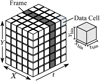 |
Fig. 1 Schematic of an EXOD data cube with dimensions X, Y, and t. A single time frame is shaded in dark grey and a single data cell with dimensions Xbin, Ybin, tbin is shown. In practice, the data cube for a single event list can contain many millions of cells depending on the binning parameters. |
2.4 Quantifying variability in the Poisson regime
For a given cell of our data cube, we make the assumption that the photon events produced are the result of a Poisson process, and thus their probability function is given by
 (1)
(1)
where N is the observed number of counts in a time and space interval, and μ the expectation value of the Poisson distribution. An important detail here is that μ is not the background expectation, but merely the expectation value of a given data cell, for example, a cell containing a non-variable source would have an expectation that is composed of the contribution from both the source and background (μ = μS + μB).
At first glance this equation would suggest that if we know the expectation (μ) of the Poisson distribution for a given data cell, one could simply calculate the probability, P(N, μ) of the N observed events having been produced by a Poisson process, finally one could simply set a threshold below which a cell would be flagged as significant.
However, as discussed in Kraft et al. (1991), classical attempts to derive confidence intervals in the regime of nonzero background have several pitfalls, and instead the authors strongly recommend using a Bayesian formalism to overcome these limitations.
2.4.1 Bayesian formalism
Adopting a Bayesian formalism, we define our null hypothesis model (θ0) as: “there is no additional transient emission on top of the background and a possible constant source”, such that the observed counts (N) are a Poisson realisation of the expectation (μ).
Our alternative hypothesis (θ1) is that the observed counts (N) are a result of an additional transient emission on top of the expectation (μ). This transient emission can also be negative (i.e. an eclipse instead of a peak), in which case the formalism is the same but with a negative amplitude, and thus some resulting formulas are slightly altered.
To compare two competing hypotheses, we define a Bayes factor B (sometimes called the odds ratio) as the ratio of the two marginal likelihoods
 (2)
(2)
where we have used Bayes’ theorem to invert the conditional probabilities. The marginal distribution of observed counts, P(N), (which would be given by p(N) = ∫ P(s)p(N s)ds) end up cancelling out to 1.
We make the assumption of a flat prior for the ratio of P(θ0)/P(θ1) = C and assume it is constant. It could be argued that this ratio is actually a function of meta-parameters (e.g. the timescale we are searching), but for the sake of simplicity and tractability of the computation, we keep it constant.
The likelihood P(N θ0), of having observed N counts given the null hypothesis (θ0) is given simply by the Poisson probability function (eq. (1)).
The posterior probability distribution, P(N θ1), of having observed N counts given the presence of a real transient on top of the expectation μ is less straight-forward. Assuming the transient has an amplitude of s, the likelihood is given by the slightly modified expression (eq. (3)):
 (3)
(3)
However, we do not know the value of s. The hypothesis θ1 takes into account all possible amplitudes. The likelihood of θ1 can thus be expressed by integrals over s. Assuming we are assessing the presence of a peak (and thus s>0), we can express it as follows:
 (4)
(4)
At this point, we have to assume a prior for the peak amplitude P(s′). The simplest is a flat prior, which can be moved out of the integral and will join the other prior of having a peak in the data. It is shown in Kraft et al. (1991) that this assumption results in negligible differences. In this case, we get
 (5)
(5)
Here, Γ(N + 1, μ) is the incomplete upper gamma function, and Q(N + 1, μ) the regularized incomplete upper gamma function. We have used Γ(N + 1) = N! for positive integers.
The Bayes factor for peaks can now be expressed as
 (6)
(6)
where K is a combination of all flat priors.
Similarly, by integrating on negative values of s, we can obtain the Bayes’ factor for eclipses:
 (7)
(7)
Here 𝒫(N + 1, μ) is the regularized incomplete lower gamma function and K′ the combination of all flat priors (a priori different from K).
At this point, assuming we have an expected value μ for the counts in a given 3D pixel of our data cube, and the actual observed counts N, we have quantified the likelihood of having a transient in the form of BPeak and BEclipse, both still containing an unknown constant prior. From a practical standpoint, we now need to determine a threshold on these values above which a pixel presents a significant departure from μ (i.e. if it can be considered variable).
2.4.2 Variability significance
To determine the correct threshold, we can use the fact that at large values of μ (say μ > 1000), a normal distribution with mean μ and standard deviation  is an accurate approximation to the Poisson distribution.
In the large count regime, it is commonplace to calculate the significance of departure from the expectation through a sigma value (σ) given by
 (8)
(8)
For example, if μ = 1000, to obtain a positive 3σ departure from μ, we would require an observed number of counts of N = 1139 or N = 870, likewise for 5σ this is N = 1237 and N = 788. We can then substitute these values for μ and N back into our formula for the Bayes’ factor (fixing K and K′ at a value of 1, since this normalization is arbitrary) to find values corresponding to a significant variability. For example, using the three-sigma upper and lower values for N we obtain
 (9)
(9)
and for five sigma, we obtain
 (10)
(10)
We can then use these threshold values of B globally, even in the small count regime, to obtain a 3 or 5 sigma equivalent score (see Fig. 2). We can verify visually that the regions of significant variability behave in a manner consistent with Poisson noise: for large counts, these regions converge with a symmetric normal departure from the diagonal N = μ, while in low counts a relatively large number of counts is required to be considered a peak, and no eclipse can be detected.
This approach is designed to detect outbursts or eclipses occurring on similar timescales to the size of the time bins. This implies two key points: firstly, this method is not well-suited for identifying low-amplitude modulations within a light curve. Secondly, to detect faint bursts effectively, the bin size should closely match the timescale of the burst, making it essential to test across many time-binning parameters.
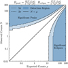 |
Fig. 2 Observed counts (N) against expected counts (μ) shown in the range 0.01–300 counts. The significant detection regions for peaks and eclipses are denoted by the dashed (3σ) and dotted (5σ) lines and are shaded in blue. These thresholds correspond to the sigma equivalent thresholds (see text). |
2.4.3 Amplitude estimation
The Bayesian formalism can also be used to estimate the parameter (s) of our model (i.e. the amplitude of the peak or eclipse). The precise computations can be found in Appendix A. It is very similar to what is usually done to estimate the brightness or upper limit of X-ray sources (e.g. Ruiz et al. 2022).
The general idea is to use the intimate link between Γ functions and Poisson statistics to provide a confidence interval for the amplitude of a transient (peak or eclipse), knowing only N and μ. After computation, we use
 (11)
(11)
and
 (12)
(12)
where Q and 𝒫 are the regularized incomplete upper and lower Gamma functions, and ULpeak( f ) and ULeclipse( f ) are the count upper limits with a probability of f (i.e. the count values compared to which the actual amplitude has a probability f to be smaller). Replacing f with the fractions 0.16, 0.5, 0.84 , we can build the 1σ confidence interval for the peak (or eclipse) amplitude.
From a practical standpoint, this computation is relatively expensive, so it is not possible to simply compute these values for the entire 3D grid and keep only the pixels for which the amplitude is non-zero at a given significance threshold. On the contrary, it is only used on the pixels that are good transient candidates, found by computing BPeak and BEclipse and keeping values above the thresholds presented in Sect. 2.4.2.
2.5 Estimating the expected emission
2.5.1 General considerations
In Sect. 2.4, we established a method for quantifying variability as a function of the observed (N) and expected (μ) counts. We now require a method for obtaining the expectation value (μ) for each cell of our data cube.
We assume that two components are combined to create the expectation value (μ). The first is the background component which is ascribed to the galactic and extra-galactic diffuse Xray emission, as well as the time varying contribution from soft proton emission originating from the sun. The second component is the contribution from the sources in the field of view of the telescope, which are assumed to be constant over the time of an observation. Any departure from the sum of these two components will be interpreted as transient behaviour – either a faint source appears from the background, or a known (brighter) source departs from its expected-constant behaviour in a given time frame.
One of the novel features of our method is the ability to detect transients within flaring bad time intervals (BTIs), which are usually discarded. These BTIs correspond to frames in which the background is much higher than for the rest of the frames. This is typically defined using an arbitrary threshold on the high energy count rate over the field of view. Other methods for fast transient detection have either neglected the variable background (e.g. Pastor-Marazuela et al. 2020; Evans et al. 2010), or used background-estimating methods that accounted for them but required more data, and so forbid smaller time binning (Ruiz et al. 2024). We wanted a method that could both account for BTIs, and go down to instrumental time binning (i.e. about 5 s). During our tests, we observed that although the distribution of the background in a single XMM-Newton observation has a spatial dependence due to effects such as observing mode, gaps between the CCDs, dead pixels & vignetting, this spatial dependence remains constant during the observation, with only its amplitude changing over time. More precisely, this spatial dependence follows one template during Good Time Intervals (GTIs) and another, spatially flatter template during BTIs. This different spatial shape is due to the flatter vignetting profile of soft protons compared to X-ray photons (e.g. Kuntz and Snowden 2023,3 Fioretti et al. 2024) This means that a pair of 2D-templates describing the background in GTIs and BTIs can be simply scaled by a constant corresponding to the background amplitude in a given time frame in order to estimate the background for each data cell. This is the main observation that drove our background-computation method. The strength of this method is that, by using the 2D templates, we input prior spatial knowledge about the background, which allows us to go down to small time binning where the data is very sparse.
2.5.2 Creating the expectation data cube
The creation of the expectation (μ) data cube is a multistep process and at a high level can be described as follows:
Calculate the background template.
- (a)
Mask the sources from the image.
- (b)
Calculate the number of counts in the background.
- (c)
Inpaint the sources (i.e. interpolate the background over the masked source areas).
- (d)
Divide the image by the total counts in the background.
- (a)
Calculate the constant-source template.
- (a)
Subtract the background contribution from (1.c) from the image.
- (b)
Mask out the background.
- (c)
Divide the image by number of effective time frames in the cube.
- (a)
Combine the source and background template to create the estimation template.
Create the expectation data cube by joining many estimation templates, each one scaled by the number of background counts in the specific frame.
A diagram of this process can be found in Fig. D.1, and further details are provided below.
First, since the vignetting is different between GTIs and BTIs, we split the observation in those two categories. We split GTIs and BTIs based on thresholds applied to the total frame count rate in high energies (10–12 keV). The threshold is set at 0.5 times the number of active instruments (e.g. 1.5 ct/s for pn, MOS1, and MOS2). Unlike standard EPIC data processing, BTIs are retained and treated separately, so precise threshold computation as is done in the standard pipeline is less critical.
Frames corresponding to BTIs and GTIs are independently summed to create separate images. Source masks are generated for each image using the standard pipeline EPIC source list, with extraction radii based on the 0.2–12.0 keV EPIC count rate (20″, 40″, and 80″ for rates <0.1, 0.1–1, and >1 counts s−1, respectively). These masked regions are inpainted using INPAINT_NS from OpenCV (Bradski 2000) to estimate the background’s spatial structure. Images are normalized by dividing by their total counts, yielding the normalized background template. Multiplying the normalized background template by the total photons contained in a single frame provides the specific frame background template, this a very good approximation of background in the actual frame, which is a Poisson realization of the frame background template.
We now seek to add the contribution from the sources in the field of view, which we model as being constant in time. For this, we mask out the background from the GTI and BTI images, leaving behind only the sources. We then calculate the net source emission by subtracting the background contribution (described in the previous paragraph) from the observed source counts. Assuming the sources are constant, the average frame emission is calculated through dividing by the total number of frames, thus obtaining the frame source template (which is identical for all frames in the data cube).
Summing the source and background templates in a given frame yields the frame expectation template. Arranging all the frame templates in time then yields the expectation data cube, in which each 3D pixel (data cell) contains the expectation value (μ) that accounts for both the background and source contribution.
Significant deviations between the observed (N) data cube and expectation (μ) data cube are interpreted as transient behaviour: either a known point-like source is not constant, and thus it will deviate in data cells from its averaged emission, or a faint transient event deviates from the background expectation in some data cells.
It is worth noting that we have only mentioned the constant emission from point-like sources. Some significant issues appear in the presence of extended sources. They are too large to be correctly inpainted using the same method as for point sources, which results in a spurious overestimation of the background. Additionally, since these sources are constant while the background is not, a large number of false positives can happen within their extent. We address these issues in post-processing (Sect. 2.7).
2.6 Benchmarking the method
Having created a method for quantifying the statistical significance in any given cell in our data cube (Sect. 2.4.2) by means of comparing it to the expected emission (Sect. 2.5), we now need to assess the sensitivity of our method via simulations.
2.6.1 Quantification of false negatives
A commonly used approach for benchmarking detection tools is to use the end-to-end X-ray telescope simulation package SIXTE (Dauser et al. 2019). However, because the main contaminants of our method are elusive instrumental effects as well as the complex temporal and spatial evolution of the background, we have opted to use real XMM-Newton observations into which synthetic bursts are added.
Synthetic bursts are modelled by specifying an amplitude, spatio-temporal position and extent. The spatial extent is modelled as a 2D normal distribution with a standard deviation set to 6.6″ to match the FWHM PSF, and the temporal extent constrained to a single time bin. The amplitude is then distributed across the data cells following these probability distributions.
We performed simulations by adding a single burst to a random position in an observation and then determining whether the burst was detected at the five-sigma level. We repeated the simulation over a grid of 10 observations, 3 time binnings (5 s, 50 s and 200 s), 15 burst amplitudes and 15 random burst positions. These values were then used to obtain constraints on the detection fraction.
Figure 3 shows the mean and standard deviation of the detection fraction as a function of the burst amplitude in counts (bottom) and count rate (top), the different lines correspond to the three different time binnings. Overall, our method is sensitive down to ∼10 photons, which is typically lower than the detection threshold for XMM-Newton observations, this is encouraging for the possibility of discovering new transients. With smaller time binning, fewer counts are necessary ( 8 at 5 s compared to 20 at 200 s for a 50% completeness), but these require much higher count rates to achieve such counts in much shorter time bins. A 90% completeness at 5σ confidence level is reached at around 10+7, 20 ± 10 and 30 ± 10 counts for the 5 s, 20 s and 200 s binning respectively (the error bars corresponding to the 1σ deviation of the detection rate over a sample of observations).
As expected, this method is more sensitive (by a factor of 3) for GTIs than for BTIs (due to the lower background levels), as can be seen in Fig. B.1. However, the method is still sensitive enough to allow for the detection of new transients in BTIs which are usually ignored in automatic processing of the archives (which under our definition represents around 20% of the archive).
An interesting side result of the benchmark presented in Fig. 3 is that it provides us with an estimate of the maximum time binning at which our method is relevant. Looking at the completeness of the 200 s-timebin peaks as a function of the amplitude in terms of counts, we see that even around 10 photons, a relatively low fraction of the peaks are detected. For an amplitude of 20 photons, the 1σ lower limit is at less than 10% completeness – but this is also enough photons for the traditional source detection pipeline to pick up this source (although 100 counts are required to perform a variability assessment).
It is important to note that this sensitivity was measured at a 5σ level, which is expected to provide us with few false positives. The 3σ completeness benchmark is shown in Fig. B.2, with as expected a higher completeness (or equivalent completeness at lower peak amplitudes). For instance, the 90% completeness counts drop to 8 2, 12 5 and 20 10 for the 5 s, 20 s and 200 s binning respectively. We however expect higher rates of false positives at a 3σ level compared to 5σ once applied to real data.
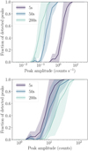 |
Fig. 3 Fraction of synthetic peaks detected with 5σ confidence threshold, as a function of the amplitude of the peak and the time binning. The amplitude here is the theoretical amplitude, before the Poisson realisation. The shaded area represents the standard deviation across different observations. Top panel: this completeness is depicted as a function of the input amplitude of the peak expressed in count rate. Bottom panel: same quantity, but expressed as a function of the input counts. |
2.6.2 Quantification of false positives
Having quantified the detection fraction (rate of false negatives), it is important to try to quantify the rate of spurious signals (false positives). There are several possible sources of false positives: the first is due to statistical variations, due to the large number of samples drawn from the underlying Poisson distribution, random fluctuations in the data may mimic true signals. The second comes from instrumental effects that are not fully accounted for in our method. The third source of spurious detections can arise from an inaccurate estimate of a data cell’s background rate.
While assessing the rate of false positives due to instrumental effects and inaccurate background estimates remains challenging, the rate of false positives arising from statistical fluctuations can be quantified through simulations.
To estimate the number of false positives caused by statistical fluctuations, we performed the following steps. First, through the process described in Sect. 2.5.2 we created data cubes of the expectation value for 20 random XMM-Newton observations across three time bin durations: (5 s, 50 s, 200 s). For each of these data cubes, we generated 120 Poisson realizations, thereby simulating a sample of 2400 observations at each time bin. These simulated observations were then processed through the EXOD detection pipeline, and the number of spurious detections arising from samples drawn in the tail of the Poisson distribution were counted.
At the 3σ detection threshold, we found that across all time binnings around 200/2400 observations ( 8.3%) led to spurious transient events, while at the 5σ threshold we did not detect any spurious detections in the simulated observations. When extrapolated to the full archive of 15 000 observations we predict a contamination of 1250 false detections at the 3σ threshold and only a handful of false positives at the 5σ level.
Do note that this only corresponds to false positives due to Poisson fluctuations, and other types of contamination will be assessed in Sect. 2.7.2.
2.7 Post-processing & Filtering
As is the nature of conducting a search for signals in such a large dataset, one is naturally confronted with many false positives which may arise from a variety of sources.
One source is simply from the extremely large number of free trials over which the search was conducted (see Sect. 2.6.2). Over all our runs we considered approximately 2.3 trillion data cells, this means that encountering events with extremely low probabilities such as to P ∼ 10−10 are not inconceivable, this would be equivalent to observing a count of N = 10 given an expectation of μ = 1 from a Poisson distribution.
Other sources of spurious signals can be caused by detector effects such as hot pixels (Sect. 2.7.2) or uneven exposure across the CCDs (see Appendix A in De Luca et al. 2021) or optical overloading due to bright stars. Bright extended sources such as supernova remnants or galaxy clusters may also cause false positive transient alerts, as well as the brightest pointsources, for which the PSF is so extended that our inpainting algorithm fails. We additionally notice that spurious signals are often found near the start and end of observations due to instrumental effects. Optical loading is present in a few detections such as 0823432701, while moving target observations such as those made of Jupiter or comet 21P/Giacobini-ZinneR 0864840301 can cause spurious signals.
Number of post-processing of detection flags and percentages as a total of the threeand five-sigma detections.
2.7.1 Detection quality flags
Table 1 shows the breakdown of the number of detections by various post-processing flags and their percentages, based on 3σ and 5σ significance levels. The table lists isolated flares (defined as alerts that were preceded and followed by 0 count bins), lastbin alerts (where a significant alert occurred in the last bin of the observation), and other critical conditions, including problematic observations, observations with more than 20 detections, and regions occurring in hot areas (Sect. 2.7.2).
2.7.2 Identification of instrumental hot areas
As previously mentioned in Sect. 2.2, previously known hot pixels on the three detectors had been already removed during the pre-processing steps when loading the event lists. However, because we are operating in previously unexplored temporal regimes, it is possible that a number of previously unknown detector quirks can contribute to false positive alerts.
To explore this effect, we took all regions detected by EXOD and transformed the coordinates into detector coordinates. Figure B.3 shows the spatial distribution of detections in the 0.2–12.0 keV band split by the three different time binnings. We observe that at the 5 s binning, there are a number of areas that contain a much higher density of regions which are likely due to intrinsic detector effects, this excludes the region that is near the centre of the detector which is where the target of the observation is usually positioned. At the 50 and 200 s binning there are fewer of these overdense regions observed, however we observe an overabundance of detections on the semicircular segment on the MOS chip that does not overlap with the pn. A line of detected regions extending over one of the pn CCDs can be seen and is due to an instrumental read-out streak caused by bright targets.
We identified 35 overdense areas at the 5 s binning, 5 areas at 50 s, and 3 areas at 200 s. In total 4890/60 127 (8.13%) (3σ) of the detected regions were flagged in the final catalogue for being potentially instrumental false-positives.
Number of detected regions for different run parameters at the three-sigma (top) and five-sigma (bottom) level.
3 Results
3.1 Overview
EXOD was run over 15 105 observations in the XMM archive. Runs were carried out for 3 different timescales: tbin = 5, 50 and 200 seconds and three different energy bands: 0.2–2.0, 2.0–12.0 and 0.2–12.0 for a total of 9 different run subsets. This resulted in 135 945 (15 105 9) total runs for a combined total of 87 billion processed photon events in 2.3 trillion data cells.
116 310/135 945 ( 85%) runs ran successfully, accounting for approximately, 12 923/15 105 observations. The remaining unsuccessful runs can be broken down into: 1228 observations did not have source lists likely due to very short exposures, 905 observations were in timing mode, 22 observations were in unsupported submodes, and finally, 27 observations failed due to edge-cases.
The spatial binning was fixed at XYbin = 20″, while the global count rate for identifying bad time intervals was set to either 0.5, 1.0 or 1.5 ct/s depending on if there were 1, 2 or 3 simultaneously observing instruments (pn, MOS1, MOS2). A detection threshold “sigma equivalent” of 3 was set for the runs, however we saved the Bayes factors so that this threshold could be later adjusted. In this section we will denote values arising from the 3 and 5 sigma populations by (3σ) and (5σ) .
3.2 Detection statistics
Across all 135 954 runs, we detected a total of 60 127 (3σ) or 11 273 (5σ) variable regions. Table 2 shows the number of detected regions separated into the three energy bands and three time binnings investigated, as well as the number of detected regions for 3 sigma (top) and 5 sigma (bottom).
To identify unique regions across our runs, we converted the RA (α) and Dec (δ) to Cartesian coordinates on a unit sphere using x = cos δ cos α, y = cos δ sin α and z = sin δ. We then used a k–d tree, a commonly used spatial clustering algorithm (Bentley 1975), to cluster together all detected regions within 20″. This clustering resulted in 32 247 (3σ) or 4083 (5σ) unique regions.
Table 3 shows the number of unique regions across our grid of run parameters, while Fig. 4 shows the sky distribution of these unique regions in galactic coordinates, where the colour map denotes the spatial density.
A clustering radius of 20″ was chosen to match the spatial binning used when creating the data cubes in EXOD, and was further motivated by the observation of a kink at this value seen when plotting the number of clusters against the clustering radius.
The percentage of peak detections found in BTIs is 22% at 3σ (26% at 5σ), which is slightly higher than the overall fraction of BTI exposure that is around 20%. This means that there is a slight bias for peak detections in BTIs, which could be due to failures in accounting for the increased background – however, the fact that there is only a few percentage difference in the fractions also shows that most of the peaks picked up by EXOD during BTIs are genuine.
EXOD found 4115 unique sources containing at least one eclipsing (dipping) bin at the 3σ threshold and 1710 at 5σ threshold. While many of these eclipses are genuine, they tend to suffer more greatly from instrumental effects than peaks. In particular, for eclipsing (dipping) detections there is a much stronger bias towards detections in BTIs with around ~60% of eclipsing detections being caught during BTIs for both the 3 and 5 sigma thresholds. This over-representation confirms that a part of them are due to limitations of our algorithm. Manual inspection of the eclipses revealed two main contamination scenarios. In the first one, if any of the CCDs turns off during a period of flaring background, this leads to a reduction of the observed counts and potentially a spurious eclipse. In the second scenario, some extended or particularly bright sources are not adequately dealt with using the filtering procedure described in Sect. 2.5.2 which leads to spurious eclipses during BTIs.
Number of unique (clustered within 20″) detected regions for different run parameters at the three-sigma (top) and five-sigma (bottom) level.
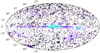 |
Fig. 4 Position of the 32 247 (3σ) unique variable regions in galactic coordinates. The colour map represents number density of transient regions. |
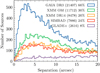 |
Fig. 5 Distribution of separations obtained from cross-matching the 32 247 EXOD unique regions against several catalogues. The numbers in brackets show the number of cross-matches that are found within 20 arcseconds for each catalogue; the percentage of the total unique regions (3σ) is also shown. |
3.3 Cross-matching with external catalogues
To enhance the characterization of EXOD sources, we crossmatched against two existing XMM-Newton catalogues 4XMMDR14 (Webb et al. 2020) (~ 650k sources) and the XMM-OM Serendipitous Source Survey Catalogue (XMM-OM-SUSS6.0) (~ 6.6m sources) (Page et al. 2012, 2023). Additionally, we crossmatched sources from EXOD with the SIMBAD astronomical database (~ 18.8m sources), (Wenger et al. 2000), Gaia DR3 (Gaia Collaboration 2023) (~ 1.8b sources) and the GLADE+ galaxy catalogue (Dálya et al. 2022) (~ 23.2 m sources), we also conduct comparisons to EXTraS (Sect. 3.3.2) and a catalogue of fast radio bursts (Sect. 3.3.1).
We selected the nearest match within 20″ which are added as columns in the final EXOD catalogue, cross-matches further than this radius are not included in the catalogue.
The distribution of separations is shown in Fig. 5, the number in brackets denoting the number of sources found within 20″ and the associated percentage of the 32 247 unique regions, we find the majority of matches peaking at an absolute separation of 3.33″. By considering only the successful matches against the 4XMM-DR14 catalogue, we estimate our positional error to be of 9.75 5.22 arcseconds (1 sigma).
This error is consistent with a simple prediction that can be made from the spatial binning of the data cube, assuming that the true position of a source can be uniformly distributed anywhere within a pixel of 20 × 20 arcsec, the 1σ error for both RA and Dec would be given by  and thus the absolute separation error can be estimated by
  .
.
By taking the successfully cross-matched sources with 4XMM-DR14, we can compare the fluxes found between the transients detected by EXOD and the standard XMM-Newton pipeline. From Fig. 6, we see that EXOD is capable of finding transient behaviour at lower flux levels than the standard pipeline. We note that this comparison only contains fluxes for previously detected pipeline sources, meaning that in reality the red histogram extends to lower fluxes. EXOD does not currently calculate the energy flux for each detection, it only provides the user with a raw photon count. This is not corrected for instance for response change across the off-axis angle, neither does it make any spectral assumption required to convert photon flux into catalogue-comparable energy flux. This is an avenue of improvement for the post-processing of EXOD alerts.
Figure 7 shows the log10 of total number of counts in each detected EXOD light curve, shown for the full population and also split by the three different time binnings investigated. The threshold on the number of counts for variability analysis for the standard XMM-Newton pipeline is set at 100 counts, we can see that we have a considerable number of light curves with fewer counts than this in our sample, further justifying the ability of EXOD to search down to lower detection limits.
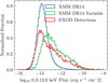 |
Fig. 6 Flux comparison between the whole XMM DR14 Catalogue (blue), variable sources in the DR14 catalogue (green), and EXOD sources with a successful 4XMM-DR14 cross-match (red). |
3.3.1 Cross-match with CHIME FRB catalogue
We also cross-matched the EXOD sources with the CHIME FRB catalogue (CHIME/FRB Collaboration 2021), which includes 536 fast radio bursts (FRBs) detected by the Canadian Hydrogen Intensity Mapping Experiment (CHIME). FRBs are extremely bright and rapid radio bursts lasting only a few milliseconds, with their origins still under debate. Notably, CHIME/FRB Collaboration (2020) reported an FRB from the galactic magnetar SGR 1935+2154, which coincided with a burst of X-ray activity (Palmer 2020). If this FRB had occurred in an external galaxy, it would share similar properties to known extragalactic FRBs, suggesting that some FRBs may be associated with X-ray transients from highly magnetized neutron stars. Our crossmatch identified 67 EXOD sources with positions consistent with 23 CHIME/FRB sources.
We find many of the bursts could be conceivably explained by other astrophysical phenomena based on their SIMBAD cross-matches, or result from spurious detections or associations, the latter which are more common due to be the large localisation uncertainties for sources in the CHIME catalogue which are around 0.26 ± 0.1 degrees (925 ± 367 arcseconds). Manual inspection of the EXOD matches, did not reveal any fast flaring behaviour similar to those seen in SGR 1935+2154, nor did we find any transients with hard spectra similar to those seen in other transient magnetars.
The weakest detections in EXOD contain 3 counts in a 5second bin, in other words, they reach a peak count rate of ~0.6 when averaged over a single 5-second bin. Using this value, we can obtain a crude estimate as to what depth was searched by EXOD for FRB counterparts, using the WebPIMMS v4.14, we converted a count rate of 0.6 in XMM/pn Thin 5’ region to 0.2– 12.0 keV flux. We used a power-law model of ~2.6, this number obtained from the average value of 16 magnetars in the McGill online magnetar catalogue (Olausen & Kaspi 2014). We used a hydrogen column density of NH = 5 1020 cm−2 as an approximate value for the sky outside the galactic plane. We obtain an absorbed flux of ~ 9 × 10⁻¹³ erg s−1 or ~ 1.4 × 10⁻¹² erg s−1 if unabsorbed.
Comparison of the number of unique sources in EXOD and EXTraS for different data subsets in EXOD and EXTraS (see Sect. 3.3.2).
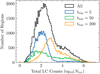 |
Fig. 7 Histogram of the log total number of counts in the light curve for all EXOD detections (3σ). |
3.3.2 Comparison to EXTraS
To date, one of the most exhaustive studies for variability in the XMM-Newton archive has been the EXTraS project: (Exploring the X-ray transient and variable sky) De Luca et al. (2021). The analysis undertaken in this paper contains partial overlap with EXTraS but also is distinct in a number of ways. One difference is the dataset, in EXTraS only data up to 3XMM-DR4 is used, meaning only 7437 observations up to December 2012 were included. By using 4XMM-DR14 our analysis includes an additional 10 years of data up to the end of December 2023. Another key difference is the temporal domain covered, as the shortest new transient discovered by EXTraS had a bin width of only 315 s, which is greater than the largest binning (200 s) we consider in this study. Despite some of these differences, we can still obtain a preliminary comparison between the transients detected with EXOD and those detected by EXTraS.
Table 4 contains the results from the cross-match performed between the sources in EXOD (3σ) & (5σ) and the sources in EXTraS (full population and variable-only4 population).
The number of overlapping observations is the intersection between the 8670 observations (3σ) (2787 at 5σ) that contained EXOD detections and the 7007 (3312 variable only) observations that contained EXTraS detections. The number of EXOD and EXTraS sources that are contained in these overlapping observations is shown in rows two and three of Table 4. The final two rows of the table display the number of sources and percentage, with (w/) cross-matches within 20″ for both EXOD and EXTraS.
We see that for the EXOD (3σ) population ~25% of sources have a cross-match in the full EXTraS catalogue. As expected, this value is similar to the percentage obtained between 4XMMDR14 and EXOD (3σ) (see legend in Fig. 5) as the sources in EXTraS closely mirror the sources in the standard pipeline catalogue. This number increases to 57% if we only include the 5σ EXOD detections.
Looking at the intersection between EXOD and the EXTraS variable sources (columns 2 and 4), we see that only around 15% of EXOD sources (3σ) are associated with a variable source in EXTraS, and conversely only 20% of variable EXTraS sources are associated with an EXOD source. This value does increase considerably for the (5σ) EXOD population to around 45%. Despite the overlap between the catalogues, we can still safely say that the variable sources detected by EXOD and EXTraS are substantially different from one another to warrant the use of our method alongside existing methodologies in the literature.
These observations suggest that the EXOD and EXTraS variable sources differ significantly. This divergence likely arises from the differing definitions of variability between EXOD and EXTraS and also from our analysis targetting shorter time intervals. These results validate our methods’ ability to uncover new transients, distinct from those identified by EXTraS and the standard XMM-Newton pipeline, justifying its use as an additional tool in X-ray variability studies.
3.3.3 Estimating the fraction of spurious cross-matches
When cross-matching catalogues from different wavelengths, a significant fraction of matches can be spurious. Taking the extreme case of cross-matching two completely independent sets of positions and uncertainties, a certain number (given roughly by the product of the sky densities of both catalogues) will overlap and thus be wrongfully associated. Taking the obtained cross-matched fraction at face value would thus lead to the wrong physical conclusion, in this example, that the two sets of coordinates are not independent.
Given the high source densities of the external catalogues we are cross-matching against, combined with the relatively large positional uncertainty of EXOD sources, we expect a certain fraction of our cross-matches to be spurious. While it may be possible to distinguish the real and spurious associations on a case-by-case basis, this is a relatively intensive process, and so we quantified these values through the use of Monte Carlo simulations.
To estimate the effect of spurious matches, we first take the catalogue we are cross-matching against and shift all positions by a specific amount in RA and Dec. This shifting serves to preserve the statistical properties (such as the sky density) of the secondary catalogue while essentially creating a new catalogue that should be completely independent of the sources in EXOD. Cross-matching with this shifted catalogue should yield fewer associations than the unshifted cross-match, the difference (excess) in the number of associations thus indicates the number of true, non-spurious matches. Repeating this process many times allows us to quantify the statistical significance of the number of true matches.
Because the sky distribution of sources is not isotropic (i.e. there is a higher density in the Galactic plane and the LMC), shifting the secondary catalogue too far would result in very dramatic changes in the number of associations which would be not representative of the underlying spurious cross-match values. Therefore, we chose to shift the coordinates of the secondary catalogue by up to ±15′ which is approximately half the EPIC field of view, this value is small enough that local statistical properties such as the sky density are maintained but large enough to suppress true associations.
We focus on the 23 769/32 247 sources (3σ) in EXOD that did not have counterparts in 4XMM-DR14 – these are the sources with the greatest uncertainty in their authenticity. We perform the aforementioned test with the SIMBAD, Gaia, and OM catalogues. For each catalogue, we shift their positions by 10 values in both RA and Dec (± 15′), each time measuring the number of associations. We then compare the distribution of these 100 samples against the number of matches obtained from the unshifted catalogue. The results of this experiment are shown in Fig. B.4), and summarized in Table 5.
As can be seen in Table 5 and Fig. B.4, the unshifted crossmatches significantly exceed the shifted cross-matches for all catalogues. Our simulation suggests that for the subset of EXOD sources with no counterparts in 4XMM-DR14, approximately half of the SIMBAD and OM associations are real and around ∼20% of the Gaia associations are real, this is expected as Gaia contains almost 1000 times the number of sources as SIMBAD and the OM catalogues.
There are two main takeaways: first, the fraction of spurious matches is large, so performing this test was essential. Secondly, even for sources not present in the DR14 catalogue, the excess is very significant. This means that these sources are most likely actual astrophysical sources. This is an essential result: it confirms that EXOD is able to detect new faint astrophysical sources, below the standard detection levels of the catalogues. Finally, the large fraction of spurious matches does not necessarily mean that these EXOD sources are spurious transients and instrumental effects, but rather that they do not have a multi-wavelength counterpart in the catalogues we have used.
Estimation of real and spurious cross-match associations.
3.4 Breakdown of SIMBAD cross-match results
Table E.1 contains the results of the cross-match of various data subsets with SIMBAD. The table is sorted by the number of each SIMBAD object classification for the full EXOD (3σ) dataset and object types that had at least 15 sources.
The other columns in the table show the results from the same cross-match but performed with different starting datasets, the number below the name of the dataset denotes the total number of sources in the population. The DR14 and DR14 (var) columns denote the results from cross-matching the whole 4XMM-D14 catalogue and only the variable sources (defined as those with SC_VAR_FLAG=True) respectively. The EXOD ∩ DR14 (⌐ var) and EXOD ∩ DR14 (var) correspond to the intersection of sources from EXOD with the non-variable and variable sources in 4XMM-DR14 respectively. Finally, the SIMBAD column shows the total number of each object classification in the SIMBAD catalogue, this number is helpful in evaluating any possible bias in the cross-matching process.
The first observation is that only a minority of sources (~ 25%) have possible SIMBAD counterparts, this is expected as the SIMBAD database only contains 18.8m sources across many wavelengths and is skewed towards bright sources that have been studied in detail, while many of the sources we have in EXOD are right at the limit of the X-ray detection limit, are new, and will not have multi-wavelength counterparts.
Of the sources that do have counterparts, we see the largest proportion (~ 4%) arising from stars. This makes sense as most stellar flares detected by EXOD will arise from nearby stars which are likely to have a SIMBAD entry. These stellar flares are also responsible for many other of the stellar classifications, for example T Tauri stars are a class of young stars and are known to be strongly variable in the X-ray and optical bands (Feigelson & Montmerle 1999).
The second most common object type in the EXOD sample would appear to be galaxies which have a similar abundance to stars with around 1200, but are noticeably lacking in sources identified as variable in the standard pipeline with only 54. Manual inspection of the light curves for these sources suggests that some of these classifications are correct, such as the known QPEs in 2MASX J02344872-441 (eRO-QPE1) (Arcodia et al. 2021) and GSN 069 (Miniutti et al. 2019). We also expect a number of these objects to be incorrect associations, owing to the relatively dense distribution of galaxies in SIMBAD. In this case, a faint source in our sample can be associated with a galaxy if there is one nearby even if it is physically independent. It is also possible that some of these associations are true, in which case further studies of short term bursts in galaxies will need to be done to identify the nature of these objects. This is beyond the scope of this current work.
Eclipsing binaries and Long Period Variable stars are also over-represented in EXOD due to large numbers of these object types existing in SIMBAD, which are a result of large catalogues of these systems being created by surveys such as Gaia (Mowlavi et al. 2023; Lebzelter et al. 2023) and others. However, the contamination rate for these classifications is lower compared to galaxies, as some of these sources do display genuine transient X-ray behaviour.
Continuing down the list, we find sub-types of galaxies and stars. We also find extended objects that are not expected to produce X-ray bursts (e.g. Part of Cloud or HII region). These are likely due either to spurious associations, or maybe extended X-ray emission that leads to issues in the EXOD pipeline as previously mentioned.
Known X-ray emitting categories in SIMBAD such as cataclysmic variables (CVs), HMXBs and the general “Xray Source” category contain fewer spurious associations as expected. This is because it is unlikely (though not impossible) that a spurious EXOD transient would be located at the position of a known X-ray source.
By looking at the intersection between EXOD sources and variable DR14 sources [EXOD DR14 (var)], we observe 2568 source. The highest fraction of common detections between the two are stars, AGNs, and CVs.
The intersection between the sources detected with EXOD and the sources in 4XMM-DR14 that are not variable [EXOD ∩ DR14 (⌐ var)] amounts to 5910 sources. These sources indicate that EXOD may be more sensitive to certain types of variability than the standard XMM pipeline. This column shows that a number of AGN-related types such as Seyferts and Quasars are identified as being variable in EXOD but not detected as such in 4XMM-DR14. The reason for this is due to the stochastic, aperiodic variability commonly seen in these sources (McHardy & Czerny 1987) leading to significant departures from the expected emission in a given time bin, while the standard χ2 variability test in the XMM pipeline is less sensitive to this type of flickering variability.
Selection of sources detected by EXOD showing novel or previously unreported variability.
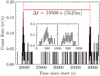 |
Fig. 8 0.2–12 keV light curve of the candidate QPE 4XMM J235440.7373019 binned at 50 s originating from the galaxy WISEA J235440.81373020.6. The inset shows zoomed-in images of 500s on the first (left) and second burst (right). |
4 Examples of variable sources detected with EXOD
In this section we will focus on a small subset of the sources that were detected by EXOD that show intriguing behaviour. Table 6 lists the sources discussed in this section and gives the 4XMM identifier if they are present in the 4XMM-DR14 catalogue, while if they are new sources detected by EXOD we provide their EXOD identifier as per IAU naming conventions. For pipeline detected sources, the mean flux from the 4XMMDR14 catalogue is shown. Note that due to the out bursting nature of these sources, the mean flux calculated over the whole observation will not well describe the peak flux or flux change during the burst. We also provide a tentative identification for the source.
4.1 A candidate QPE in 4XMM J235440.7-373019?
EXOD detected a transient at RA=23h54m40.8s Dec = –37d30m21s in obsid 0884250101 taken on 27th May 2021 during a 53ks observation of the exoplanet LTT 9779b.
The source shows two distinct soft bursts lasting ~1000s (~15m) each separated by ~19 500 s (~ 5h25m) (see Fig. 8 and is associated with the galaxy WISEA J235440.81-373020.6. When binned at 200 s the mean count rate during the ∼20ks preceding the first burst was found to be ∼0.002 ct/s while the first burst reached a maximum count rate of ∼0.28 ct/s This represents a factor ∼100 increase in the source count rate.
Visual inspection of images taken by the VLT Survey Telescope (Shanks et al. 2015) suggest that this galaxy could potentially be two overlapping galaxies; however, higher resolution imaging and or spectroscopy is required to confirm this.
The source is present in the 4XMM-DR14 catalogue with a mean flux of 1.01 × 10⁻¹⁴ ± 3.57 × 10⁻¹⁵ erg s−1 and was also previously identified as variable.
The spectra of the bursts (Fig. 9) appear to be consistent with a black body of temperature kT =0.25 ± 0.002 keV with a scaling constant K = (1.57 ± 0.65) × 10−6, and column density of nH = (9.92 ± 9.93) × 1020 cm−2 and a fit statistic of χ2 = 14.15/18 0.79. In the absence of any accurate distance measurements, a crude luminosity estimate of 1041–1042 erg s−1 is obtained assuming distances in the range 100–300 Mpc. The hydrogen column density at the position of the source obtained via the HEASARC nH tool5 is ~ 9.7 × 1019 cm−2.
These values are broadly similar to known QPEs; however, with only two observed bursts and a scarcity of the available data, further investigations are needed to confirm the nature of the source.
 |
Fig. 9 Spectrum of candidate QPE, 4XMM J235440.7-373019 extracted during the two outbursts. Values of nH are given in cm−2, and of kT in keV. |
4.2 A magnetar candidate 4XMM J175136.9-275858?
EXOD detected a hard transient outburst towards the end of observation 0886121001, at the coordinates 17h51m36.91s – 27:58:58.98. The source had previously been detected in the XMM catalogue as 4XMM J175136.9-275858 and was also flagged as variable. The source is located towards the Galactic centre, and no known optical counterparts are found within the X-ray position’s error circle.
The source would appear to share many similar spectral and timing properties to known magnetars. Specifically, the hard spectrum in both quiescence and during the 1ks outburst, combined with the estimated luminosity of L ~ 1033 erg s−1 in quiescence and L ~ 1035 erg s−1 during the outburst (assuming a distance to the Galactic centre of ~7 kpc) is a factor 100 above the brightest stellar flares. SXFTs can also be ruled out as any supergiant companion at these distances should be clearly visible in other wavelengths. A search for pulsations was conducted but proved inconclusive, and a full investigation into this source can be found in Webbe et al. (2025).
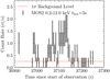 |
Fig. 10 0.2–12.0 keV MOS2 light curve of EXOD J174037.7-304544 binned at 5 seconds. |
4.3 A previously unknown hard X-ray burst near the Tornado
On the 5th March 2006, XMM-Newton made a 61ks observation (obsid: 0301730101) of G357.7-0.1, a dual-lobed radio and Xray structure referred to as the Tornado (Helfand & Becker 1985; Gaensler et al. 2003). Approximately ~ 37 ks into the observation, EXOD detected a large X-ray burst in all three time binnings (5 s, 50 s & 200 s) and in both the full (0.2–12.0 keV) and hard (2.0–12.0 keV) energy bands. The source was extremely off-axis and thus only in the field of view of MOS2 (thick filter) during the outburst. The burst is faintly visible in the pipeline processed image; however, it was not identified as a source by the standardized pipeline. The observation was reprocessed from the raw CCF files using a circular extraction region for both the source and background, with approximately half of the region being inside the CCD in both cases. The RMF and ARF were created from the spectra extracted in these regions using the rmfgen and arfgen respectively.
By manually estimating the centroid of the source, we obtain coordinates of 17:40:38.9590 –30:45:54.724 and estimate approximately 100 counts present within the burst.
Visual inspection of the field in the optical wavelengths shows no plausible counterparts, due to the high extinction present in the Galactic plane at these wavelengths. In the NearInfrared (2MASS colour 10 806–23 552 Å) (Skrutskie et al. 2006) several plausible counterparts are observed, the nearest of these is denoted 17403893-3045540 at a separation of 0.79″ and has magnitudes of J = 18.3, H = 14.8, Ks = 13.2, the next closest is 17403844-3045584 at a separation of 7.64″ with J = 17.183, H = 12.806, Ks = 10.533.
The post-processed light curve is shown in Fig. 10, which is binned at 5 second intervals with the 1σ background assuming a Poisson process at 0.25 ct/s shown as a red dotted line. The burst is very bright, ~1.8 raw counts per second at its peak, this value is estimated to be closer to ~8 counts per second once absolute corrections are included (vignetting and PSF). We note that the shape of the burst appears to not have the typical fast rise/exponential decay that is observed in Type-I bursts, but somewhat more of a symmetrical profile, although with only ~100 total counts it is difficult to assess the true shape of the burst.
We fit the spectrum extracted during the burst (see Fig. 11) with several models in xspec (see Table C) using the cstat statistic to account for the low number of counts.
We used both a single and double absorbed power-law model, commonly applied to XRBs, neutron stars or Type-I X-ray bursts, as well as two models that model the emission from hot, diffuse gas that may be more commonly associated with flaring young stellar objects. Based on the fits in Table C it was not possible to determine which model was preferred. The 0.2–12.0 keV absorbed flux derived using the doubly absorbed power law model gave 1 × 10⁻⁹ erg cm−2 s−1, with a 1-sigma uncertainty range of 2 × 10⁻¹⁰ to 1 × 10⁻⁸ erg cm−2 s−1. The hydrogen column density at the position of the source via the HEASARC nH tool is 1.3 1022 cm−2.
Assuming a distance of 8 kpc (approximately the distance to the Galactic centre) we obtain a luminosity of 1.9 ± 0.4 × 1036 erg s−1.
This luminosity equates to approximately ~ 0.01 LEdd (Eddington) for a 1.4 M⊙ NS. However, the observed spectrum is significantly harder than is usually seen in type-I X-ray bursts which usually have temperatures of around 0.2 keV (Galloway et al. 2020).
Assuming a closer distance of 100 pc, the luminosity is around ~ 1.2 × 1033 erg s−1, with the 1 sigma range being between ~ 2.4 × 1032–1.2 1034 erg s−1. This would place it above the luminosity range for stellar flares, but within the luminosity range of XRBs, CVs and SFXTs (see Sect. 1).
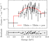 |
Fig. 11 Spectrum of EXOD J174037.7-304544, extracted during the outburst, binned at minimum of three counts per bin and fit using a doubly absorbed power law. |
4.4 A possible X-ray counterpart to a galactic radio pulsar
EXOD J174603.8-284931 is an example of one of the fainter sources that EXOD can detect that are not detected by the standard pipeline. Its light curve is consistent with a steady background (at a rate of about 2 × 10⁻³ photons per second in EXOD pixels), apart from one 5-second-long time bin containing 4 hard photons. This corresponds to a 3.8σ detection in the EXOD framework. Out of these photons, three were detected by EPIC pn in adjacent pixels and time bins (less than one second apart), and the fourth photon was detected by EPIC MOS2, all with energies between 4 and 7 keV. This indicates that it is unlikely to be an instrumental effect (which tend to happen in a single instrument and in a single pixel). While not extremely significant in itself, this detection is interesting because of its multi-wavelength context.
This detection is consistent with the position of PSR J17462849 (at 11″), a known radio pulsar in the Galactic centre. The statistics of the pulsars detected by EXOD are shown in Table E.1: out of 3739 SIMBAD pulsars, EXOD detected 23. From those, 22 are in DR14, and 7 are flagged as variable by DR14. EXOD J174603.8-284931 is the only EXOD pulsar that is not in DR14 – which is understandable given its faintness. The very low counts prevent us from performing a deep spectral study; however, we can roughly estimate the luminosity of the burst (using the WebPIMMS tool6). The radio-measured dispersion measure of PSR J1746-2849 is significant, at DM ≈ 1330 pc cm−3 (Abbate et al. 2023), corresponding to NH ≈ 4 × 1022 cm−2 (using the conversion formula from He et al. 2013). Assuming a rate of about 4 counts/s in the 4–7 keV band (which is what was observed), and an absorbed power-law spectrum with Γ = 1.7 and NH = 4 × 1022 cm−2, this leads to a 0.2–12 keV flux of around 10−10 erg s−1 cm−2, and thus a luminosity of ~ 1035 erg s−1. This is consistent with reconnection in the magnetosphere of the pulsar, with a surface magnetic field of B ≈ 4 × 10¹² G from the ATNF catalogue (Manchester et al. 2005).
Although tentative, this detection of a possible X-ray counterpart to a radio pulsar proves the potential of EXOD to detect faint sources, beyond the capabilities of the usual XMM-Newton pipeline, and thus provides us with potentially new scientific discoveries from existing archives.
4.5 Eclipse detections
Manual inspection of the eclipsing–dipping detections from EXOD yielded many previously known real astrophysical phenomena that were previously identified as variable by the standard XMM-Newton pipeline. Examples include the modulations observed in the magnetic CV RX J0838.7-2827 (see Rea et al. 2017) and the eclipsing LMXB AX J1745.6-2901 (Maeda et al. 1996) detected in 26 different observations.
One example of an eclipsing detection that was not previously identified as variable by the standard pipeline is XMMSL1 J063045.9-603110. This source was initially detected in a slew observation (Read et al. 2011), and displayed a 5σ threshold eclipse during the last 4000 seconds of observation 0679381201. Initially theorized to be a TDE (Mainetti et al. 2016) the source was reclassified as a Nova following optical spectroscopy by Oliveira et al. (2017). This specific eclipse was also picked up by the EXTraS project (De Luca et al. 2016; Kovacˇevic’ et al. 2022).
4.6 BTI detections and a candidate FXT
Since the standard pipeline removes Bad Time Intervals from the data products, any transients that happen during those will be missed, even if they are bright. We show in Table 7 some examples of transients detected by EXOD during periods of high background that were not identified as variable by the standard pipeline – most of these are stellar flares in already X-ray emitting stars, but the last source is completely new.
EXOD J034111.1-284816 displayed a soft (0.2–2.0 keV) burst lasting around ~75 s, approximately 26ks into observation 0653770101 right during a Bad Time Interval, peaking at around 0.5 counts per second (Fig. 12). Assuming a soft thermal emission (with for instance a black-body temperature of 100 eV), this leads to a peak flux of the order of magnitude of 10−13 erg s−1. Our cross-matching routine revealed no nearby sources in 4XMM-DR14, SIMBAD or Gaia, although it may be associated with the AllWise source J034111.03-284815.8 and two faint PanSTARRS sources at a r-band magnitude of about 21 – all of them falling in the error region. It is difficult to confirm the nature of this object without more data, but the timing and spectral properties as well as the large X-rays–to–optical ratio makes it a credible FXT candidate.
Examples of transients detected by EXOD during periods of high background activity (BTIs) not identified as variable by the standard pipeline.
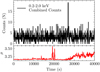 |
Fig. 12 Top: 0.2–2.0 keV light curve for EXOD J034111.1-284816 binned at 50 seconds; the significant burst is around the ~26ks mark and lasts around ~75 seconds. The counts are combined from all three instruments MOS1, MOS2 & pn. Bottom: Background expectation counts over the course of observation 0653770101. |
5 Discussion
5.1 Strengths and weaknesses
EXOD demonstrates several key strengths that make it a powerful tool for the search of rapid X-ray transients. The Bayesian framework, which relies on comparisons with an informed template, proves to be robust even in the presence of a both temporally and spatially varying background. The statistical specification for the quantification of sensitivity in the Poisson regime enables the detection of transient events in very short time windows that are dominated by shot noise, and permits searching down to deeper limits than other methodologies that assume a Gaussian distribution of counts (Masias et al. 2012).
EXOD also allows the detection of both positive and negative departures from the expected emission, that is to say it is simultaneously sensitive to both outbursts and eclipses, the latter of which are often overlooked in classical source detection algorithms. Finally, EXOD is computationally efficient with average processing time for a single observation in this work taking 3.3 seconds over 12 cores with our largest bottleneck being memory allocation of the data cubes. The rapid computational time allows for the exploration of many parameter combinations such as binning and timescales, which make it well suited for large-scale searches for transient events.
EXOD does have certain limitations, as previously mentioned. EXOD may find spurious detections in the presence of extended sources with diffuse emission. As was mentioned at the end of Sect. 2.5.2, extended sources lead to spurious transients detection within their extent. Despite this, it is still possible for EXOD to detect true signals within these diffuse regions, hence we only flag these detections and do not throw them out. EXOD is also not particularly effective in identifying long-term lowamplitude variability trends, as it relies on a local comparison in a specific time bin. However, this type of variability is identified in the XMM-Newton pipeline analysis using the chi-squared tests. Similarly, EXOD is not directly sensitive to structured variability such as repeating signals; however, this could be implemented as a post-processing step. EXOD remains vulnerable to unpredictable forms of instrumental noise such as hot pixel events or optical loading, but we have flagged all currently known issues in post-processing. Finally, since many of our detections are fast and faint, containing only a few photons in a single bin, standard X-ray analysis methods such as the production of spectra or analysis of light curves is often unfeasible. This means that we must turn to analysis of the transient population as a whole and rely on external information such as those obtained via cross-matching in order to overcome these limitations.
Despite these weaknesses, EXOD can and has been successful in identifying reliable variability in sources that were previously considered non-variable, as well as finding new sources in previously discarded times of high background.
5.2 Planned future developments for EXOD
5.2.1 Searching at the position of known objects
Instead of attempting to pick out all significant signals in the field of view, a possible alternative approach to finding new transients would be to simply extract photon events at the position of known sources. For example, if one was interested in finding weak TDE or QPEs, then simply extracting photon events at the position of known galaxies could prove fruitful.
5.2.2 Investigation of other energy bands
This study has only investigated the variability in three broad XMM energy ranges 0.2–12.0, 0.2–2.0 & 2.0–12.0 keV. Due to the computational efficiency of EXOD it would not be unreasonable to perform searches over smaller, targeted bands to search for instances of variability arising from specific spectral emission or absorption lines. This may be especially useful when extending our method to future instruments with very high X-ray spectral resolutions such as Athena.
5.2.3 Adaptive time binning
EXOD currently only tests for significance in individual time bins set by the tbin parameter, which for this work has been set to 5, 50 and 200 s. It is possible however to miss transients that are not at timescales that are explicitly searched for. For example, a transient with a duration of 10 seconds may be too faint to be evaluated as significant at 50 seconds binning, but also may have its photons split over two bins at 5 second binning and therefore not reach the significance threshold in either bin.
One possible solution would be to have an initially lower detection threshold (say 2σ), which would first identify these low-significance events, then extract the photon events in a small spacial and temporal region surrounding the candidate, finally we can then rapidly iterate to find out which time binning (and possibly other parameters) would provide the largest significance for the event. This method would allow for greater flexibility in the types of detected transients and would avoid having to re-run the whole pipeline on the entire archive each time a new set of parameters was investigated.
5.2.4 Improved position estimation
In a similar fashion to the temporal dimension, it is possible that some post-processing steps might improve the precision of the detections in the spatial dimension. For now, the position of a source is taken as the center of the corresponding 20′ × 20″ cell. We could for instance compute the centroid of the photons in the flaring frame in order to get a better estimate of the position of the source.
5.2.5 Advanced light curve post-processing
Recent advances in machine learning methods such as neural networks and their variants, have proven to be effective methods in the modelling, classification and even prediction of future variability trends. However, many of these supervised machine learning methods require well-labelled training sets in order to work effectively. Unsupervised methods such as clustering or anomaly detection may also prove to be effective in flagging novel variability patterns. To date we have performed some preliminary experiments using these methods, and we have reason to believe that the dataset created through EXOD has strong potential for exploitation via these methods.
6 Conclusions
In this paper we have presented the development of the EPIC XMM Outburst Detector (EXOD). Through the creation of a novel detection method, we have improved the algorithm’s sensitivity in the low-count (Poisson) regime and are now able to probe previously discarded bad time intervals (BTIs). We highlighted four noteworthy sources, including a possible candidate quasi-periodic eruption (QPE) found with EXOD that may be of particular interest to the scientific community.
EXOD was run successfully on 12 926 observations in the XMM-Newton archive, which includes data up to December 2023. We investigated three different energy bands: a full band (0.2–12.0 keV), a soft band (0.2–2.0 keV), and a hard band (2.0– 12.0 keV) as well as three different time bins (5 s, 50 s & 200 s), with the aim of capturing a wide range of transient phenomena.
EXOD initially yielded 32 247 unique variable regions in 12 926 observations at the 3σ detection level and 4083 unique regions at the 5σ level. At the 3σ detection level, 8478, or around one-quarter of the sources detected by EXOD are associated with a previously known source in the latest XMM-Newton catalogue (4XMM-DR14). At the 5σ detection level, there are 1 766/4083 ( 43%). Conversely, the number of new sources (without a 4XMM-DR14 counterpart) are 23 769 ( 74%) at the 3σ level and 2317 ( 57%) at the 5σ level.
4XMM-DR14 contains 6311 variable sources, while the total number of sources detected by EXOD at the three-sigma level is approximately five times this number. Of the 8478 EXOD sources with an associated XMM pipeline detection, 2568 ( 30%) had been previously flagged as variable in the standard pipeline, while 5910 ( 70%) had not.
Because EXOD is specifically adapted for the search of rapid transient behaviour and is also sensitive to transient events at the limit of the detector sensitivity, it is expected that the population detected by EXOD only contains a partial overlap with the standard catalogue as both of these regions of parameter space were known to be overlooked during the creation of the standardized pipeline.
Future papers will focus on the detailed characterisation of newly identified transients, as well as further refinement of the detection algorithm in order to enhance its detection sensitivity and reduce the number of false-positive alerts.
Data availability
We provide two catalogues that were created using EXOD on the XMM-Newton archive, one for detections and one for unique (spatially clustered) sources. They are provided as Flexible Image Transport System (FITS) files. The EXOD detections catalogue contains 60 127 rows and 27 columns, while the unique source catalogue contains 32 247 rows and 40 columns. These Tables are available in electronic form at the CDS via anonymous ftp to cdsarc.cds.unistra.fr (130.79.128.5) or via https://cdsarc.cds.unistra.fr/viz-bin/cat/J/A+A/697/A50 (Ochsenbein et al. 2000), as well as on the EXOD site: http://xmm-ssc.irap.omp.eu/exod which contains further documentation on the tables.
Acknowledgements
This project has received funding from the European Union’s Horizon 2020 research and innovation programme under grant agreement number 101004168, the XMM2ATHENA project (Webb et al. 2023). NAW and RW also acknowledge support from the CNES. IT acknowledges support by Deutsches Zentrum für Luftund Raumfahrt (DLR) through grant 50 OX 2301. This research has made use of data obtained from the 4XMM XMM-Newton serendipitous source catalogue compiled by the 10 institutes of the XMM-Newton Survey Science Centre selected by ESA (Webb et al. 2020). This research has also made use of the SIMBAD database, operated at CDS, Strasbourg, France (Wenger et al. 2000). This research has made use of the NASA/IPAC Extragalactic Database (NED), which is funded by the National Aeronautics and Space Administration and operated by the California Institute of Technology. (Helou et al. 1991).
Appendix A Parameter estimation
Let us assume that a pixel has been flagged as variable, and we want to estimate the properties of the associated burst or eclipse. The idea is that we will compute an upper limit value UL, which is to be larger than the peak amplitude at a given confidence level. Let us for instance consider the median – in this case, the peak amplitude is below UL at a 50% confidence level. Computing the corresponding UL for 16% and 84% allows a 1σ confidence interval for the peak to be built. In order to compute these UL values, we integrate the Poisson statistics up to UL, so that we recovered the intended fraction of the total integral over all possible peak amplitudes:
 (A.1)
(A.1)
where f is the intended fraction. Assuming Poisson statistics, an expected rate of μ and a flat prior for the peak amplitudes,
 (A.2)
(A.2)
 (A.3)
(A.3)
 (A.4)
(A.4)
 (A.5)
(A.5)
 (A.6)
(A.6)
 (A.7)
(A.7)
 (A.8)
(A.8)
![Mathematical equation: $UL+\mu=\mathcal{P}^{-1}\left[N+1,\mathcal{P}(N+1,\mu)+{\rm f}\times\mathcal{Q}(N+1,\mu)\right]$](/articles/aa/full_html/2025/05/aa53647-24/aa53647-24-eq24.png) (A.9)
(A.9)
with Q and 𝒫 the regularized upper and lower incomplete gamma function. By using Eq. A.9 and taking f = {0.16,0.5,0.84}, we can retrieve the 1σ lower and upper limits as well as the median of the estimated flux. This only requires using the expected and observed counts, μ and N respectively.
It works similarly for eclipses, the main difference being that all integrals are on a finite support (between 0 and the expected rate μ):
 (A.10)
 (A.11)
 (A.12)
![Mathematical equation: $\mu-UL = \mathcal{P}^{-1}\left[N+1,\mathcal{P}(N+1,\mu)-{\rm f}\times\mathcal{P}(N+1,\mu)\right]$](/articles/aa/full_html/2025/05/aa53647-24/aa53647-24-eq28.png) (A.13)
(A.13)
Appendix B Additional benchmarking statistics
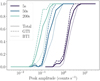 |
Fig. B.1 Detection fraction at 5σ for GTI, BTI, and total frames. |
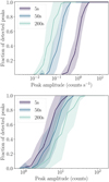 |
Fig. B.2 Detection fraction for different time binnings evaluated at the (3σ) sensitivity. |
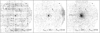 |
Fig. B.3 Spatial distribution of transient detections (3σ) in the 0.2–12.0 keV energy band in detector coordinates. The three panels correspond to the different time binning: 5s, 50s, and 200s. A number of areas of overdensity can be seen; detections located in these areas are flagged. |
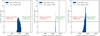 |
Fig. B.4 Estimation of the fraction of spurious associations between new EXOD sources (not in DR14) and the SIMBAD, Gaia, and OM catalogues. In each panel, the blue histogram corresponds to the results of the Monte Carlo shifted cross-match method, and the black dotted line to the number of associations in the true dataset. The red and green lines show the numbers of spurious matches and real matches, respectively. |
Appendix C Spectral fits for Tornado burst
| Model | Component | Parameter | Unit | Value | Error | χ2/DoF & P-value |
|---|---|---|---|---|---|---|
| TBabs*Powerlaw | TBabs | nH | 1022 | 16.77 | ±3.96 | 50.70/36 ~ 1.41 |
| Powerlaw | Γ | 2.60 | ±0.80 | 0.0251 | ||
| Powerlaw | norm | 0.155 | ±0.222 | |||
| TBabs*TBabs*Powerlaw | TBabs(1) | nH | 1022 | 1.30 | frozen | 50.69/36 ~ 1.41 |
| TBabs(2) | nH | 1022 | 15.45 | ±3.95 | 0.0252 | |
| Powerlaw | Γ | 2.59 | ±0.80 | |||
| Powerlaw | norm | 0.154 | ±0.220 | |||
| TBabs*Raymond | TBabs | nH | 1022 | 15.06 | ±2.88 | 51.09/36 ∼ 1.42 |
| Raymond | kT | keV | 4.09 | ±2.08 | 0.0231 | |
| Raymond | Abundance | 0.30 | frozen | |||
| Raymond | Redshift | 0.00 | frozen | |||
| Raymond | norm | 0.185 | ±0.112 | |||
| TBabs*Apec | TBabs | nH | 1022 | 15.28 | ±2.96 | 51.46/36 ∼ 1.43 |
| Apec | kT | keV | 3.87 | 1.90 | 0.0213 | |
| Apec | Abundance | 0.30 | frozen | |||
| Apec | Redshift | 0.00 | frozen | |||
| Apec | norm | 0.193 | ±0.123 | |||
Appendix D Diagram of the creation of the expectation emission
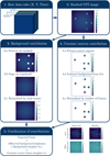 |
Fig. D.1 Diagram of the steps used to estimate the expectation value for each cell of the data cube (for details, see Sect. 2.5.2) |
Appendix E Breakdown of SIMBAD cross-match results
Source classifications numbering 15 or more obtained by cross-matching sources in the full EXOD (3σ) catalogue with SIMBAD.
References
- Abbate, F., Noutsos, A., Desvignes, G., et al. 2023, MNRAS, 524, 2966 [Google Scholar]
- Aizu, K. 1973, Progr. Theoret. Phys., 49, 1184 [NASA ADS] [CrossRef] [Google Scholar]
- Alp, D., & Larsson, J., 2020, ApJ, 896, 39 [NASA ADS] [CrossRef] [Google Scholar]
- Arcodia, R., Merloni, A., Nandra, K., et al. 2021, Nature, 592, 704 [NASA ADS] [CrossRef] [Google Scholar]
- Arcodia, R., Miniutti, G., Ponti, G., et al. 2022, A&A, 662, A49 [NASA ADS] [CrossRef] [EDP Sciences] [Google Scholar]
- Arcodia, R., Liu, Z., Merloni, A., et al. 2024, A&A, 684, A64 [NASA ADS] [CrossRef] [EDP Sciences] [Google Scholar]
- Bagnoli, T., in’t Zand, J. J. M., D’Angelo, C. R., & Galloway, D. K., 2015, MNRAS, 449, 268 [NASA ADS] [CrossRef] [Google Scholar]
- Bentley, J. L., 1975, Commun. ACM, 18, 509 [CrossRef] [Google Scholar]
- Berger, E., 2014, ARA&A, 52, 43 [CrossRef] [Google Scholar]
- Bradski, G., 2000, Dr. Dobb’s Journal of Software Tools, The OpenCV Library, 120, 122 [Google Scholar]
- Cash, W., 1979, ApJ, 228, 939 [Google Scholar]
- Chakraborty, J., Kara, E., Masterson, M., et al. 2021, ApJ, 921, L40 [NASA ADS] [CrossRef] [Google Scholar]
- Chartas, G., Kochanek, C. S., Dai, X., Poindexter, S., & Garmire, G., 2009, ApJ, 693, 174 [Google Scholar]
- CHIME/FRB Collaboration (Andersen, B. C., et al.) 2020, Nature, 587, 54 [Google Scholar]
- CHIME/FRB Collaboration (Amiri, M., et al.) 2021, ApJS, 257, 59 [NASA ADS] [CrossRef] [Google Scholar]
- Dálya, G., Díaz, R., Bouchet, F. R., et al. 2022, MNRAS, 514, 1403 [CrossRef] [Google Scholar]
- Dauser, T., Falkner, S., Lorenz, M., et al. 2019, A&A, 630, A66 [NASA ADS] [CrossRef] [EDP Sciences] [Google Scholar]
- D’Avanzo, P., Salvaterra, R., Sbarufatti, B., et al. 2012, MNRAS, 425, 506 [CrossRef] [Google Scholar]
- De Luca, A., Salvaterra, R., Tiengo, A., et al. 2016, in Astrophysics and Space Science Proceedings, 42, The Universe of Digital Sky Surveys, eds. N. R. Napolitano, G. Longo, M. Marconi, M. Paolillo, … E. Iodice, 291 [Google Scholar]
- De Luca, A., Salvaterra, R., Belfiore, A., et al. 2021, A&A, 650, A167 [NASA ADS] [CrossRef] [EDP Sciences] [Google Scholar]
- Duncan, R. C., & Thompson, C., 1992, ApJ, 392, L9 [Google Scholar]
- Eappachen, D., Jonker, P. G., Quirola-Vásquez, J., et al. 2024, MNRAS, 527, 11823 [Google Scholar]
- Evans, I. N., Primini, F. A., Glotfelty, K. J., et al. 2010, ApJS, 189, 37 [NASA ADS] [CrossRef] [Google Scholar]
- Fabbiano, G., 2006, ARA&A, 44, 323 [NASA ADS] [CrossRef] [Google Scholar]
- Feigelson, E. D., & Montmerle, T., 1999, ARA&A, 37, 363 [Google Scholar]
- Fioretti, V., Mineo, T., Lotti, S., et al. 2024, A&A, 691, A229 [NASA ADS] [CrossRef] [EDP Sciences] [Google Scholar]
- Foschini, L., Pian, E., Maraschi, L., et al. 2006, A&A, 450, 77 [NASA ADS] [CrossRef] [EDP Sciences] [Google Scholar]
- Gaensler, B. M., Fogel, J. K. J., Slane, P. O., et al. 2003, ApJ, 594, L35 [Google Scholar]
- Gaia Collaboration (A. Vallenari, et al.) 2023, A&A, 674, A1 [NASA ADS] [CrossRef] [EDP Sciences] [Google Scholar]
- Galloway, D. K., & Keek, L., 2021, in Astrophysics and Space Science Library, 461, Timing Neutron Stars: Pulsations, Oscillations and Explosions, eds. T. M. Belloni, M. M. Méndez, & C. Zhang, 209 [NASA ADS] [CrossRef] [Google Scholar]
- Galloway, D. K., in’t Zand, J., Chenevez, J., et al. 2020, ApJS, 249, 32 [NASA ADS] [CrossRef] [Google Scholar]
- Giustini, M., Miniutti, G., & Saxton, R. D., 2020, A&A, 636, L2 [NASA ADS] [CrossRef] [EDP Sciences] [Google Scholar]
- Guolo, M., Pasham, D. R., Zajacˇek, M., et al. 2024, Nat. Astron., 8, 347 [Google Scholar]
- Hayashida, M., Nalewajko, K., Madejski, G. M., et al. 2015, ApJ, 807, 79 [Google Scholar]
- He, C., Ng, C. Y., & Kaspi, V. M., 2013, ApJ, 768, 64 [NASA ADS] [CrossRef] [Google Scholar]
- Helfand, D. J., & Becker, R. H., 1985, Nature, 313, 118 [Google Scholar]
- Helou, G., Madore, B. F., Schmitz, M., et al. 1991, in Astrophysics and Space Science Library, 171, Databases and On-line Data in Astronomy, eds. M. A. Albrecht, & D. Egret, 89 [Google Scholar]
- Imanishi, K., Nakajima, H., Tsujimoto, M., Koyama, K., & Tsuboi, Y., 2003, PASJ, 55, 653 [NASA ADS] [CrossRef] [Google Scholar]
- Jansen, F., Lumb, D., Altieri, B., et al. 2001, A&A, 365, L1 [NASA ADS] [CrossRef] [EDP Sciences] [Google Scholar]
- Jonker, P. G., Glennie, A., Heida, M., et al. 2013, ApJ, 779, 14 [NASA ADS] [CrossRef] [Google Scholar]
- Kapanadze, B., Dorner, D., Vercellone, S., et al. 2016, ApJ, 831, 102 [NASA ADS] [CrossRef] [Google Scholar]
- Kaspi, V. M., & Beloborodov, A. M., 2017, ARA&A, 55, 261 [Google Scholar]
- Kato, M., Saio, H., & Hachisu, I., 2015, ApJ, 808, 52 [Google Scholar]
- King, A., Lasota, J.-P., & Middleton, M., 2023, New A Rev., 96, 101672 [NASA ADS] [CrossRef] [Google Scholar]
- König, O., Wilms, J., Arcodia, R., et al. 2022, Nature, 605, 248 [CrossRef] [Google Scholar]
- Kovacˇevic’, M., Pasquato, M., Marelli, M., et al. 2022, A&A, 659, A66 [NASA ADS] [CrossRef] [EDP Sciences] [Google Scholar]
- Kowalski, A. F., 2024, Liv. Rev. Sol. Phys., 21, 1 [NASA ADS] [CrossRef] [Google Scholar]
- Kraft, R. P., Burrows, D. N., & Nousek, J. A., 1991, ApJ, 374, 344 [Google Scholar]
- Kumar, P., & Zhang, B., 2015, Phys. Rep., 561, 1 [Google Scholar]
- Kuulkers, E., den Hartog, P. R., in’t Zand, J. J. M., et al. 2003, A&A, 399, 663 [NASA ADS] [CrossRef] [EDP Sciences] [Google Scholar]
- Kuulkers, E., Norton, A., Schwope, A., & Warner, B., 2010, in Compact Stellar X-ray Sources, eds. Lewin, W., & van der Klis, M., 421 [Google Scholar]
- Lebzelter, T., Mowlavi, N., Lecoeur-Taibi, I., et al. 2023, A&A, 674, A15 [NASA ADS] [CrossRef] [EDP Sciences] [Google Scholar]
- Lewin, W. H. G., & van der Klis, M., 2006, Compact stellar X-ray sources, Cambridge Astrophysics Series, 39 (Cambridge, UK: Cambridge University Press) [CrossRef] [Google Scholar]
- Lichti, G. G., Bottacini, E., Ajello, M., et al. 2008, A&A, 486, 721 [NASA ADS] [CrossRef] [EDP Sciences] [Google Scholar]
- Linial, I., & Quataert, E., 2024, MNRAS, 527, 4317 [Google Scholar]
- Maeda, Y., Koyama, K., Sakano, M., Takeshima, T., & Yamauchi, S., 1996, PASJ, 48, 417 [NASA ADS] [Google Scholar]
- Maguire, K., Eracleous, M., Jonker, P. G., MacLeod, M., & Rosswog, S., 2020, Space Sci. Rev., 216, 39 [NASA ADS] [CrossRef] [Google Scholar]
- Mainetti, D., Campana, S., & Colpi, M., 2016, A&A, 592, A41 [NASA ADS] [CrossRef] [EDP Sciences] [Google Scholar]
- Manchester, R. N., Hobbs, G. B., Teoh, A., & Hobbs, M., 2005, AJ, 129, 1993 [Google Scholar]
- Masias, M., Freixenet, J., Lladó, X., & Peracaula, M., 2012, MNRAS, 422, 1674 [NASA ADS] [CrossRef] [Google Scholar]
- McHardy, I., & Czerny, B., 1987, Nature, 325, 696 [NASA ADS] [CrossRef] [Google Scholar]
- Miniutti, G., Saxton, R. D., Giustini, M., et al. 2019, Nature, 573, 381 [Google Scholar]
- Miniutti, G., Giustini, M., Arcodia, R., et al. 2023, A&A, 674, L1 [NASA ADS] [CrossRef] [EDP Sciences] [Google Scholar]
- Morgan, C. W., Hainline, L. J., Chen, B., et al. 2012, ApJ, 756, 52 [Google Scholar]
- Mowlavi, N., Holl, B., Lecoeur-Taïbi, I., et al. 2023, A&A, 674, A16 [NASA ADS] [CrossRef] [EDP Sciences] [Google Scholar]
- Nicholl, M., Pasham, D. R., Mummery, A., et al. 2024, Nature, 634, 804 [CrossRef] [Google Scholar]
- Ochsenbein, F., Bauer, P., & Marcout, J., 2000, A&AS, 143, 23 [NASA ADS] [CrossRef] [EDP Sciences] [Google Scholar]
- Olausen, S. A., & Kaspi, V. M., 2014, ApJS, 212, 6 [Google Scholar]
- Oliveira, A. S., Rodrigues, C. V., Cieslinski, D., et al. 2017, AJ, 153, 144 [NASA ADS] [CrossRef] [Google Scholar]
- Page, K. L., & Shaw, A. W., 2022, in Handbook of X-ray and Gamma-ray Astrophysics, eds. Bambi, C., & Sangangelo, A., 107 [Google Scholar]
- Page, M. J., Brindle, C., Talavera, A., et al. 2012, MNRAS, 426, 903 [NASA ADS] [CrossRef] [Google Scholar]
- Page, M. J., Brindle, C., Talavera, A., et al. 2023, VizieR Online Data Catalog: XMM-OM Serendipitous Source Survey Catalogue (XMM-SUSS6.0) (Page+, 2023), VizieR On-line Data Catalog: II/378. Originally published in: 2012MNRAS.426.903P [Google Scholar]
- Palmer, D. M., 2020, The Astronomer’s Telegram, 13675, 1 [Google Scholar]
- Pastor-Marazuela, I., Webb, N. A., Wojtowicz, D. T., & van Leeuwen, J., 2020, A&A, 640, A124 [EDP Sciences] [Google Scholar]
- Pye, J. P., Rosen, S., Fyfe, D., & Schröder, A. C., 2015, A&A, 581, A28 [NASA ADS] [CrossRef] [EDP Sciences] [Google Scholar]
- Quintin, E., Webb, N. A., Guillot, S., et al. 2023, A&A, 675, A152 [NASA ADS] [CrossRef] [EDP Sciences] [Google Scholar]
- Quirola-Vásquez, J., Bauer, F. E., Jonker, P. G., et al. 2022, A&A, 663, A168 [NASA ADS] [CrossRef] [EDP Sciences] [Google Scholar]
- Rea, N., Coti Zelati, F., Esposito, P., et al. 2017, MNRAS, 471, 2902 [NASA ADS] [CrossRef] [Google Scholar]
- Read, A. M., Saxton, R. D., & Esquej, P., 2011, ATel, 3811, 1 [NASA ADS] [Google Scholar]
- Rees, M. J., 1988, Nature, 333, 523 [Google Scholar]
- Ridnaia, A., Svinkin, D., Frederiks, D., et al. 2021, Nat. Astron., 5, 372 [NASA ADS] [CrossRef] [Google Scholar]
- Romano, P., Evans, P. A., Bozzo, E., et al. 2023, A&A, 670, A127 [NASA ADS] [CrossRef] [EDP Sciences] [Google Scholar]
- Rosen, S. R., Webb, N. A., Watson, M. G., et al. 2016, A&A, 590, A1 [NASA ADS] [CrossRef] [EDP Sciences] [Google Scholar]
- Ruiz, A., Georgakakis, A., Gerakakis, S., et al. 2022, MNRAS, 511, 4265 [NASA ADS] [CrossRef] [Google Scholar]
- Ruiz, A., Georgakakis, A., Georgantopoulos, I., et al. 2024, MNRAS, 527, 3674 [Google Scholar]
- Saxton, R., Komossa, S., Auchettl, K., & Jonker, P. G., 2021, Space Sci. Rev., 217, 18 [NASA ADS] [CrossRef] [Google Scholar]
- Schwope, A. D., Schwarz, R., Sirk, M., & Howell, S. B., 2001, A&A, 375, 419 [NASA ADS] [CrossRef] [EDP Sciences] [Google Scholar]
- Schwope, A. D., Knauff, K., Kurpas, J., et al. 2024, A&A, 690, A243 [NASA ADS] [CrossRef] [EDP Sciences] [Google Scholar]
- Shanks, T., Metcalfe, N., Chehade, B., et al. 2015, MNRAS, 451, 4238 [NASA ADS] [CrossRef] [Google Scholar]
- Sidoli, L., 2013, arXiv e-prints [arXiv:1301.7574] [Google Scholar]
- Sidoli, L., 2017, in XII Multifrequency Behaviour of High Energy Cosmic Sources Workshop (MULTIF2017), 52 [Google Scholar]
- Skrutskie, M. F., Cutri, R. M., Stiening, R., et al. 2006, AJ, 131, 1163 [NASA ADS] [CrossRef] [Google Scholar]
- Sridhar, N., Metzger, B. D., Beniamini, P., et al. 2021, ApJ, 917, 13 [NASA ADS] [CrossRef] [Google Scholar]
- Srivastav, S., Chen, T. W., Gillanders, J. H., et al. 2025, ApJ, 978, L21 [Google Scholar]
- Strüder, L., Aschenbach, B., Bräuninger, H., et al. 2001a, A&A, 375, L5 [CrossRef] [EDP Sciences] [Google Scholar]
- Strüder, L., Briel, U., Dennerl, K., et al. 2001b, A&A, 365, L18 [Google Scholar]
- Suleimanov, V. F., Doroshenko, V., & Werner, K., 2022, MNRAS, 511, 4937 [NASA ADS] [CrossRef] [Google Scholar]
- Sun, H., Liu, H.-Y., Pan, H.-W., et al. 2022, ApJ, 927, 224 [NASA ADS] [CrossRef] [Google Scholar]
- Troja, E., Piro, L., van Eerten, H., et al. 2017, Nature, 551, 71 [NASA ADS] [CrossRef] [Google Scholar]
- Turner, M. J. L., Abbey, A., Arnaud, M., et al. 2001, A&A, 365, L27 [CrossRef] [EDP Sciences] [Google Scholar]
- Turolla, R., Zane, S., & Watts, A. L., 2015, Rep. Progr. Phys., 78, 116901 [Google Scholar]
- Warner, B., 1995, Cataclysmic variable stars, 28 [Google Scholar]
- Watson, M. G., Schröder, A. C., Fyfe, D., et al. 2009, A&A, 493, 339 [NASA ADS] [CrossRef] [EDP Sciences] [Google Scholar]
- Waxman, E., & Katz, B., 2017, in Handbook of Supernovae, eds. Alsabti, A. W., & Murdin, P., 967 [CrossRef] [Google Scholar]
- Webb, N. A., Coriat, M., Traulsen, I., et al. 2020, A&A, 641, A136 [NASA ADS] [CrossRef] [EDP Sciences] [Google Scholar]
- Webb, N. A., Carrera, F. J., Schwope, A., et al. 2023, Astron. Nachr., 344, e20220102 [Google Scholar]
- Webbe, R., & Young, A. J., 2023, MNRAS, 518, 3428 [Google Scholar]
- Webbe, R., Khan, N., Webb, N. A., & Quintin, E., 2025, MNRAS, submitted [Google Scholar]
- Wenger, M., Ochsenbein, F., Egret, D., et al. 2000, A&AS, 143, 9 [NASA ADS] [CrossRef] [EDP Sciences] [Google Scholar]
- Zhang, X., Xiong, D.-r., Gao, Q.-g., et al. 2024, MNRAS, 529, 3699 [NASA ADS] [CrossRef] [Google Scholar]
XMM-CCF-REL-0399.
Variable sources in EXTraS were defined as those with UB_LC500_CO_PVAL < 1 × 10⁻⁵, see De Luca et al. (2021).
All Tables
Number of post-processing of detection flags and percentages as a total of the threeand five-sigma detections.
Number of detected regions for different run parameters at the three-sigma (top) and five-sigma (bottom) level.
Number of unique (clustered within 20″) detected regions for different run parameters at the three-sigma (top) and five-sigma (bottom) level.
Comparison of the number of unique sources in EXOD and EXTraS for different data subsets in EXOD and EXTraS (see Sect. 3.3.2).
Selection of sources detected by EXOD showing novel or previously unreported variability.
Examples of transients detected by EXOD during periods of high background activity (BTIs) not identified as variable by the standard pipeline.
Source classifications numbering 15 or more obtained by cross-matching sources in the full EXOD (3σ) catalogue with SIMBAD.
All Figures
|
Fig. 1 Schematic of an EXOD data cube with dimensions X, Y, and t. A single time frame is shaded in dark grey and a single data cell with dimensions Xbin, Ybin, tbin is shown. In practice, the data cube for a single event list can contain many millions of cells depending on the binning parameters. |
| In the text | |
|
Fig. 2 Observed counts (N) against expected counts (μ) shown in the range 0.01–300 counts. The significant detection regions for peaks and eclipses are denoted by the dashed (3σ) and dotted (5σ) lines and are shaded in blue. These thresholds correspond to the sigma equivalent thresholds (see text). |
| In the text | |
|
Fig. 3 Fraction of synthetic peaks detected with 5σ confidence threshold, as a function of the amplitude of the peak and the time binning. The amplitude here is the theoretical amplitude, before the Poisson realisation. The shaded area represents the standard deviation across different observations. Top panel: this completeness is depicted as a function of the input amplitude of the peak expressed in count rate. Bottom panel: same quantity, but expressed as a function of the input counts. |
| In the text | |
|
Fig. 4 Position of the 32 247 (3σ) unique variable regions in galactic coordinates. The colour map represents number density of transient regions. |
| In the text | |
|
Fig. 5 Distribution of separations obtained from cross-matching the 32 247 EXOD unique regions against several catalogues. The numbers in brackets show the number of cross-matches that are found within 20 arcseconds for each catalogue; the percentage of the total unique regions (3σ) is also shown. |
| In the text | |
|
Fig. 6 Flux comparison between the whole XMM DR14 Catalogue (blue), variable sources in the DR14 catalogue (green), and EXOD sources with a successful 4XMM-DR14 cross-match (red). |
| In the text | |
|
Fig. 7 Histogram of the log total number of counts in the light curve for all EXOD detections (3σ). |
| In the text | |
|
Fig. 8 0.2–12 keV light curve of the candidate QPE 4XMM J235440.7373019 binned at 50 s originating from the galaxy WISEA J235440.81373020.6. The inset shows zoomed-in images of 500s on the first (left) and second burst (right). |
| In the text | |
|
Fig. 9 Spectrum of candidate QPE, 4XMM J235440.7-373019 extracted during the two outbursts. Values of nH are given in cm−2, and of kT in keV. |
| In the text | |
|
Fig. 10 0.2–12.0 keV MOS2 light curve of EXOD J174037.7-304544 binned at 5 seconds. |
| In the text | |
|
Fig. 11 Spectrum of EXOD J174037.7-304544, extracted during the outburst, binned at minimum of three counts per bin and fit using a doubly absorbed power law. |
| In the text | |
|
Fig. 12 Top: 0.2–2.0 keV light curve for EXOD J034111.1-284816 binned at 50 seconds; the significant burst is around the ~26ks mark and lasts around ~75 seconds. The counts are combined from all three instruments MOS1, MOS2 & pn. Bottom: Background expectation counts over the course of observation 0653770101. |
| In the text | |
|
Fig. B.1 Detection fraction at 5σ for GTI, BTI, and total frames. |
| In the text | |
|
Fig. B.2 Detection fraction for different time binnings evaluated at the (3σ) sensitivity. |
| In the text | |
|
Fig. B.3 Spatial distribution of transient detections (3σ) in the 0.2–12.0 keV energy band in detector coordinates. The three panels correspond to the different time binning: 5s, 50s, and 200s. A number of areas of overdensity can be seen; detections located in these areas are flagged. |
| In the text | |
|
Fig. B.4 Estimation of the fraction of spurious associations between new EXOD sources (not in DR14) and the SIMBAD, Gaia, and OM catalogues. In each panel, the blue histogram corresponds to the results of the Monte Carlo shifted cross-match method, and the black dotted line to the number of associations in the true dataset. The red and green lines show the numbers of spurious matches and real matches, respectively. |
| In the text | |
|
Fig. D.1 Diagram of the steps used to estimate the expectation value for each cell of the data cube (for details, see Sect. 2.5.2) |
| In the text | |
Current usage metrics show cumulative count of Article Views (full-text article views including HTML views, PDF and ePub downloads, according to the available data) and Abstracts Views on Vision4Press platform.
Data correspond to usage on the plateform after 2015. The current usage metrics is available 48-96 hours after online publication and is updated daily on week days.
Initial download of the metrics may take a while.