| Issue |
A&A
Volume 696, April 2025
|
|
|---|---|---|
| Article Number | A167 | |
| Number of page(s) | 8 | |
| Section | Stellar structure and evolution | |
| DOI | https://doi.org/10.1051/0004-6361/202553768 | |
| Published online | 17 April 2025 | |
4XMM J181330.1−175110: A new supergiant fast X-ray transient
1
Istituto Nazionale di Astrofisica, Istituto di Astrofisica Spaziale e Fisica Cosmica di Milano, via A. Corti 12, 20133 Milano, Italy
2
Department of Physics and Center for Astrophysics and Space Science, University of California at San Diego, 9500 Gilman Drive, La Jolla, CA 92093, USA
⋆ Corresponding author: This email address is being protected from spambots. You need JavaScript enabled to view it.
Received:
15
January
2025
Accepted:
26
February
2025
Abstract
Context. Supergiant fast X-ray transients (SFXTs) are a subclass of high-mass X-ray binaries (HMXBs) in which a compact object accretes part of the clumpy wind of the blue supergiant companion, triggering series of brief X-ray flares lasting a few kiloseconds. Currently, only about 15 SFXTs are known.
Aims. The EXTraS (Exploring the X-ray Transient and variable Sky) catalog provides the timing signatures of every source observed by the EPIC instrument onboard XMM-Newton. Among the most peculiar sources in terms of variability, we identified a new member of the SFXT family: 4XMM J181330.1−175110 (J1813).
Methods. We analyzed all publicly available XMM-Newton, Chandra, Swift, and NuSTAR data pointed at the J1813 position to determine the source’s duty cycle and to provide a comprehensive description of its timing and spectral behavior during its active phase. Additionally, we searched for the optical and infrared counterpart of the X-ray source in public databases and fitted its spectral energy distribution (SED).
Results. The optical-to-mid infrared SED of J1813 is consistent with a highly absorbed (AV ∼ 38) B0 star at ∼10 kpc. During its X-ray active phase, the source is characterized by continuous thousands seconds-long flares with peak luminosities (2–12 keV) ranging from 1034 to 4 × 1035 erg s−1. Its X-ray spectrum is consistent with a high-absorbed power-law model with NH ∼ 1.8 × 1023 cm−2 and Γ ∼ 1.66. No spectral variability was observed as a function of time or flux. J1813 is in a quiescent state ∼60% of the time, with an upper-limit luminosity of 8 × 1032 erg s−1 (at 10 kpc), implying an observed long-term X-ray flux variability > 500.
Conclusions. The optical counterpart alone indicates J1813 is an HMXB. Its transient nature, duty cycle, the amplitude of observed X-ray variability, the shape and luminosity of the X-ray flares – and the lack of known X-ray outbursts (> 1036 erg s−1) – strongly support the identification of J1813 as an SFXT.
Key words: stars: neutron / supergiants / X-rays: binaries / X-rays: individuals: 4XMM J181330.1−175110
© The Authors 2025
 Open Access article, published by EDP Sciences, under the terms of the Creative Commons Attribution License (https://creativecommons.org/licenses/by/4.0), which permits unrestricted use, distribution, and reproduction in any medium, provided the original work is properly cited.
This article is published in open access under the Subscribe to Open model. This email address is being protected from spambots. You need JavaScript enabled to view it. to support open access publication.
1. Introduction
High-mass X-ray binaries (HMXBs; Kretschmar et al. 2019; Fornasini et al. 2023 for the most recent reviews) are binary systems composed of a compact object, usually a neutron star (NS), accreting matter from the strong wind of the massive stellar companion. Depending on the spectral type and luminosity class of the donor (an O- or a B-type supergiant or a nonsupergiant Be star), HMXBs divide into supergiant HMXBs (SgXRBs) and Be X-ray binaries (BeXRBs). While, in BeXRBs, the massive companion rotates fast and expels material via a dense, equatorial decretion disk, in SgXRBs the outflowing wind is supersonic and approximately spherical. Most BeXRBs (Reig 2011) show aperiodic (type II, giant outbursts) and/or periodic (type I outbursts, repeating on the orbital period timescale) luminous X-ray outbursts. During type I outbursts, triggered when the NS is closer to the periastron passage and the Be decretion disk, the peak X-ray luminosity is around 1037 erg s−1, while during type II, giant outbursts it is close to the Eddington limit (1038 erg s−1). While Type I outbursts last about 20–30% of the orbital period, Type II ones can cover a number of orbital periods of the system. In BeXRBs, especially during type II outbursts, the transfer of matter onto the NS forms an accretion disk, while the SgXRBs are thought to be wind-fed sources. SgXRBs (Martínez-Núñez et al. 2017) are equally divided (for the number of members) in persistent and transient sources. The members of the latter (transient SgXRBs); they were discovered by the INTEGRAL satellite 20 years ago (Sguera et al. 2005, 2006; Negueruela et al. 2006) and display extreme properties. They shine at an X-ray luminosity level similar to persistent SgXRBs (a few 1036 erg s−1) only during short flares (those lasting only hundreds to thousands of seconds), with a duty cycle (fraction of time spent in these bright flares) of less than 5% (Sidoli & Paizis 2018). These flares are part of shorter (a few days, at most) and less luminous outbursts than BeXRBs. SFXTs are believed to host wind-fed NSs, which spend most of their time in a low luminosity state, below 1034 erg s−1. Their lowest X-ray luminosity can be as low as a few 1031 erg s−1 (Sidoli et al. 2021, 2023).
The physical driver (the neutron star magnetic field, its rotational period, the properties of the captured wind material from the supergiant companion, or the interplay of all these together) of the SFXT phenomenology is still highly debated in the literature. Therefore, the discovery of new members of the class is an important step in defining the average behavior of this subclass and comparing the population with predictions of different theoretical models (Bozzo et al. 2008; Shakura et al. 2013, 2014; Martínez-Núñez et al. 2017; Kretschmar et al. 2019).
A search in the X-ray archives for sources exhibiting pronounced short-term variability is undoubtedly the most promising method for discovering new members of these classes of objects. Among the various X-ray catalogs available, EXTraS stands out as the most powerful tool for such searches. The EXTraS project1 (De Luca et al. 2017) extracted the light curves of all sources observed by the European Photon Imaging Camera (EPIC) aboard the XMM-Newton spacecraft, which is one of the most sensitive X-ray telescopes ever built, with a large effective area, and over 20 years of available data. The main goal of the project is to characterize the variability of these sources. In recent years, we have been enhancing the capabilities of EXTraS in terms of both detection and characterization of source variability, extending the analysis to the most recent datasets. A small fraction of unpublished sources exhibiting extreme temporal features (e.g., a high number of Bayesian blocks or a peculiar shape of the cumulative light curve) have caught our attention. Among these, we report here on an unidentified source, 4XMM J181330.1−175110 (hereafter J1813), whose transient activity was serendipitously detected by XMM-Newton during a long observation and subsequently discovered thanks to the EXTraS project.
In this paper we report on the analysis of the available X-ray data (Sects. 2,3) and optical to mid-infrared (MIR) (Sect. 4). This leads us to propose an identification og J1813 with a new HMXB, in particular with an SFXT (Sect. 5).
2. Observations and data reduction
The sky position of J1813 was serendipitously covered by numerous observations from soft X-ray telescopes due to its proximity to the well-known energetic pulsar PSR J1813−1749 (see e.g., Gotthelf & Halpern 2009), its pulsar wind nebula, and the associated supernova remnant (approximately 1 7 away). Given the relative brightness of the nearby pulsar system, this paper utilizes only datasets from X-ray telescopes operating in imaging mode with sufficiently good angular resolution. For instance, we did not consider data from NICER (Gendreau et al. 2012), Suzaku (Mitsuda et al. 2007), or continuous clocking mode data from Chandra (Garmire et al. 2003). Additionally, we did not consider Swift-XRT observations, where J1813 is not detected and the observations are too short to provide scientific relevance for computing the source’s duty cycle, with an upper limit exceeding 5 × 10⁻¹³ erg cm−2 s−1. It is worth noting that these short observations cover a total exposure time of 8 ks and therefore are negligible. Table 1 presents the observations used in this paper, along with their main characteristics. As a final consideration, the XMM-Newton and Swift-XRT observations are contaminated by relatively faint straylight annuli from the low-mass X-ray binary GX 13+1, located 45′ away; however, this contamination does not affect the position of J1813 or any of the analyses presented in this paper.
X-ray observations.
The most accurate X-ray position of J1813 is derived from the Chandra Source Catalog (CSC) 2.1 (Evans et al. 2024), located at RA(J2000.0) = 18h13m30 17, Dec=−17°51′10
 3 (with a 0.30″ 1σ statistical plus systematic error). This position is consistent with that from the XMM-Newton Source Catalog 3XMM-DR14 (Webb et al. 2020).
For most of the X-ray analysis in this work, we used HEASoft (Nasa High Energy Astrophysics Science Archive Research Center (Heasarc) 2014) v.6.34, CIAO (Fruscione et al. 2006) v.4.16, and SAS (Gabriel et al. 2004) v.20.0.0.
For the XMM-Newton analysis, the event files were barycentered using the SAS tool barycen. Proton flares did not significantly affect the analyzed observations. We extracted source events from a circle with a radius of 25″ centered on the source position and background events from a nearby 50″-radius circle, also with similar contamination from the nearby PSR J1813−1749 nebula. It is noteworthy that in the longest observation, 0552790101, which was the only one with a detection, the position of J1813 was covered only by MOS cameras.
For the MOS spectral analysis of this observation, we extracted photons in the 0.3–12 keV energy range, with patterns 0–12, and only during the ‘active’ phase (see Sect. 3.1). The XMM-Newton temporal analysis was carried out using the EXTraS tools (De Luca et al. 2021; Marelli et al., in prep.) in the 2–12 keV energy band, due to its highly absorbed spectrum (see Sect. 3.2). EXTraS light curves from the two MOS cameras were binned using the same time bins (beginning with the zero XMM-Newton reference time), and therefore the count rate of each bin was converted to flux using the best-fitted spectrum (see Sect. 3.2). Finally, we calculated the weighted mean, per bin, of the flux curves of MOS1 and MOS2 to obtain the final light curve, as previously done in Marelli et al. (2017, 2018) and De Luca et al. (2020, 2022).
For the Chandra analysis, we extracted source events from a circle with a radius of 2″ centered on the source position and background events from a nearby 20″-radius circle with similar contamination from the nearby PSR J1813−1749 system. Again, we extracted photons in the 2–10 keV energy range for the Chandra timing analysis of J1813.
3. X-ray data analysis
3.1. Temporal analysis
As described in Sect. 2, we constructed the 2–12 keV XMM-Newton flux curve of J1813 (obs. id 0552790101) using EXTraS tools and taking into account the contributions from the two MOS cameras (Fig. 1). During the first 61.5 ks of observation (before T0 = MJD 51224.39856 = 35458500 s, in XMM-Newton time), the source was in a quiescent state and compatible with no flux. For the remaining 37.5 ks of the observation, the curve exhibits an apparent and bright flaring behavior, with the brightest flare reaching ∼2 × 10⁻¹¹ erg cm−2 s−1 (assuming the spectral fit derived in Sect. 3.2).
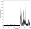 |
Fig. 1. EXTraS light curve of J1813 in the 2–12 keV energy band, 250 s time bin, T0 = 354548500. The dotted red line marks the end of the quiescent phase. |
Focusing on the quiescent state of J1813, we extracted the 2–10 keV XMM-Newton image, pattern 0–12, from the two MOS cameras, as shown in Fig. 2. The source detection procedure using the SAS tool edetect chain, performed in a single band with both XMM-Newton cameras, does not detect J1813. We computed the 3σ upper limit using the definition of signal-to-noise and a source-free region conservatively for a single camera, yielding an upper limit count rate of ∼10−3 counts s−1. This is in agreement with the count rate of the faintest source detected at > 3σ by edetect chain, which is 8 ± 2 × 10⁻³ counts s−1. Using the source spectrum from Sect. 3.2, we obtain a 3σ upper limit on the absorbed flux (2–12 keV) for the quiescent state of ∼5 × 10⁻¹⁴ erg cm−2 s−1.
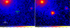 |
Fig. 2. XMM-Newton exposure-corrected image of J1813 (2–12 keV energy band, observation 0552790101) in counts ks−1 arcsec−2. Left panel: quiescent state, with T < 354610080; right panel: active state, with T > 354610080. |
During the active state, the temporal behavior of J1813 resembles a series of fast rise, exponential decay (FRED) flares, with maximum fluxes ranging from ∼2 × 10⁻¹² erg cm−2 s−1 to ∼2 × 10⁻¹¹ erg cm−2 s−1. Figure 3 (left panel) shows the cumulative light curve of events from the source region. This representation clearly marks the onset of the active state at t = T0 + 61.5 ks. Additionally, there is some indication of a different nonflaring, active “intermediate” state between T0 + 84 ks and T0 + 93 ks, where the slope appears uniform and lies between the quiescent and flaring states. Figure 3 (right panel) presents the flux curve during the active state, which remains roughly constant and nonzero. A constant fit of the “intermediate” state (in blue in Fig. 3) provides an acceptable model (null hypothesis probability, nhp = 0.30) with a flux of 5.3 ± 1.0 × 10⁻¹³ erg cm−2 s−1. However, we cannot exclude the possibility that this state consists of one or more small flares (similar to those observed in the Chandra data) and/or represents the tail end of previous flares.
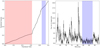 |
Fig. 3. Left panel: cumulative curve of the events taken from the XMM-Newton region around J1813 in the 2–12 keV energy band and the cuts described in Sect. 2 (we note that it is not background subtracted). The red area marks the quiescent state; the blue area marks the possible active, nonflaring “intermediate” state. Right panel: zoom of the EXTraS flux curve, shown in Fig. 1, with only the active part of the curve (T0+61500 s). The blue area is the same as in the left panel. |
To investigate this further, we attempted to fit the flux curve of the active state with a series of FRED flares. As shown in Fig. 3, most of the flares are not isolated. Therefore, we created a segmentation of data with Scargle’s Bayesian blocks (Scargle et al. 2013), using the same events we used to create the cumulative curve. In this case, the lack of the background subtraction is not relevant since it is almost constant. This resulted in a curve with five (single or double-peaked) separated bumps. Thus, we divided the EXTraS curve into the five corresponding time intervals (denoted by dotted vertical lines in Fig. 4), each one containing a bump in the Bayesian blocks curve. For each interval, we fitted one or more FRED models, using the fewest possible number of components to achieve an acceptable (3σ) fit. The only exceptions were the sixth and eighth flares: due to their sharpness, we used a simpler Gaussian model instead. This analysis resulted in the identification of ten distinct flares. Finally, using the best-fitting parameters from each interval as starting points, we performed a simultaneous fit with 38 free parameters. The resulting fit is statistically acceptable, with χ2 = 146.9 for 111 degrees of freedom (d.o.f.), which corresponds to an nhp of 1.3 × 10⁻². This appears to be the minimum number of flares required to adequately (3σ) fit the active part of the XMM-Newton flux curve. Table 2 lists the best-fitting parameters and Fig. 4 displays the corresponding fit. Since most of the flares are well defined, with at most a minor contamination from the others, there is no degeneration in the parameters and each flare is well constrained. The only exception is flare 7: basically, this flare is necessary to represent the nonflaring “intermediate” state between T0 + 84 ks and T0 + 93 ks, it is not well constrained (e.g., it can be replaced by a constant term during that period, with variations of the nearby FRED flares), and it has parameters quite different to the others. So, although the entire active state can be described by a series of FRED flares, we cannot exclude the possibility that flare 7 is the sum of two or more shorter flares and/or the “constant” term that dominates in that particular period.
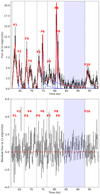 |
Fig. 4. Active part of the XMM-Newton EXTraS flux curve (from T0+61500 s), as in Fig. 3, right panel. Upper panel: flux curve (in black) plus the best-fitted model described in Sect. 3.1 (in red), which is composed of a series of ten different flares (in blue). Lower panel: residual curve of the model reported in the upper panel. |
Parameters of the flux curve fitting.
The Chandra flux curves (Fig. 5) display a behavior similar to the XMM-Newton one: two of them consist of a series of FRED-like flares, with maximum fluxes ranging from ∼5 × 10⁻¹³ erg cm−2 s−1 to ∼2 × 10⁻¹² erg cm−2 s−1. In the remaining one, observation id 17440, we observe a decrease in flux (compatible with the end of a flare) followed by ∼10 ks of quiescence – compatible (within 1σ) with the noise and incompatible (3σ) with the first part of the observation. A source detection during this last period using the CIAO tool wavdetect does not yield a detection at the position of J1813. Applying the same method as for XMM-Newton, we obtain a 3σ upper limit of ∼8 × 10⁻⁴ counts s−1. This translates into the lowest upper limit on the absorbed flux (2–12 keV) for the quiescent state of ∼4 × 10⁻¹⁴ erg cm−2 s−1 (a luminosity of 8 × 1032 erg s−1 at 10 kpc).
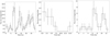 |
Fig. 5. Chandra flux curves taken in the 2–10 keV energy range. The count rate was converted into 2–12 keV flux using the best-fitted spectrum (see Sect. 3.2). Left panel: observation 6685, 1 ks time bin, and T0 = 274669518; central panel: observation 17440, 2 ks time bin, and T0 = 581548320; right panel: observation 17695, 1 ks time bin, and T0 = 580947681. |
Taking into account the observations reported in Sect. 2 and the considerations above, we can compute the duty cycle of J1813, i.e., the percentage of time spent by the source above a certain flux. Over 219 ks of total exposure, the source was in an active state (i.e., a flaring state with a flux of at least a few 10−13 erg cm−2 s−1 up to a few 10−11 erg cm−2 s−1) for approximately 87.5 ks, which is about 40% of the time. During the remaining 60% of the time, the source was in a quiescent state, with a 3σ upper limit flux of 4 × 10⁻¹⁴ erg cm−2 s−1.
Finally, we investigated the hard X-ray band, searching for possible bursts. No transient hard X-ray source (20–100 keV) has been reported at the J1813 position. We note that J1813 is located only 1.7 arcmin offset from the hard X-ray source IGR J18135−1751, a persistent source (supernova remnant, pulsar and/or pulsar wind nebula) showing a flux of 1.4 mCrab (about 1.1 × 10⁻¹¹ erg cm−2 s−1; 20–40 keV; Bird et al. 2016). Its positional error radius with IBIS-ISGRI is 1.4 arcmin (90% c.l.) and its proximity to J1813 hampers any detection of J1813 with INTEGRAL at similar hard X-ray fluxes. In the case of an SFXT outburst, with a much brighter (ten times or larger) flux (i.e., with a luminosity of about 1036 erg s−1, as usually shown by SFXTs at their flare peak), it might have been detected (although proper simulations would be needed to quantify this statement). However, no such activity has ever been reported in the literature, to the best of our knowledge. It is worth mentioning that the Bird et al. (2016) catalog also performs a search for transient sources on many different timescales in INTEGRAL data, reporting no hard X-ray sources at the XMM-Newton position. Since 2016, no publication or telegram has reported any transient source consistent with J1813. In the Swift-BAT catalogs the only detected source is IGR J18135−1751 (also known as Swift J1813.6−1753; Krimm et al. 2013; Oh et al. 2018).
3.2. Spectroscopy
As described in Sect. 2, we extracted the background-subtracted spectra of J1813 from the XMM-Newton observation 0552790101 and the Chandra observation 6685 – the only datasets that allow for spectral analysis, due to their having sufficient statistics. For the XMM-Newton observation, we applied a time cut to match the active state of J1813 (T > 354610080), as reported in Sect. 3.1 and shown in Fig. 3 (right panel). For this analysis, we relied on 1004, 1066, and 149 background-subtracted counts from the MOS1 and MOS2 XMM-Newton cameras and Chandra, respectively. We allowed the normalization of the different instruments to vary freely to account for cross-calibration differences and, in the case of the Chandra spectrum, the differing overall flux.
We obtained a good fit using the absorbed power-law model tbabs*powerlaw (abundances and cross sections, respectively, from Wilms et al. 2000; Verner et al. 1996), with a χ2 of 106.74 for 100 d.o.f., resulting in an nhp = 0.30. The best-fitted values are NH = (1.78 ± 0.15)×1023 cm−2 and Γ = 1.66 ± 0.20 (1σ errors). The absorbed 0.2–12 keV XMM-Newton flux is (2.10 erg cm−2 s−1, which translates into an unabsorbed flux of (7.19
 erg cm−2 s−1. Similarly, the absorbed 0.3–10 Chandra flux is (2.55
 erg cm−2 s−1, which translates into an unabsorbed flux of (1.38
 erg cm−2 s−1.
To search for possible spectral variations during the active phase over time, we used the XMM-Newton data to study the variation of the hardness ratio (HR), defined as the counts in a hard energy band over the counts in a soft energy band, as a function of time. As a first attempt, we produced standard background-subtracted light curves in the 2–5 keV (soft band) and 5–12 keV (hard band) energy bands (pattern 0–12) from the MOS1 and MOS2 cameras. We created an HR curve as the sum of the counts from both cameras in the hard band divided by the sum of the counts in the soft band, with appropriate error propagation. We used a bin size of 1 ks to achieve acceptable χ2 statistics and reasonable error bars. A fit with a constant yielded an acceptable result, with χ2 = 54.3, 36 d.o.f., and nhp = 0.0252. Next, we produced a similar HR curve using the flux curves from EXTraS in the bands 2–4.5 and 4.5–12 keV (EXTraS can only utilize the standard XMM-Newton energy bands, as defined in the 3XMM catalog). Again, we obtained an acceptable constant fit, with χ2 = 52.6, 36 d.o.f., and nhp = 0.037. Thus, we do not observe any appreciable variation in J1813’s spectrum over time.
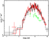 |
Fig. 6. Total spectrum of J1813. The black and red points are from MOS1 and MOS2 of XMM-Newton obs. 0552790101, respectively, while the green ones are from the Chandra obs. 6685. We also report the best-fitted model, as described in Sect. 3.2. |
We also searched for possible spectral variations during the active phase of the XMM-Newton observation as a function of flux. For each MOS camera, we extracted two spectra based on the cuts described above and an additional temporal cut: the “quiet” spectrum was taken when the EXTraS flux curve described in Sect. 3.1 (Fig. 3) had a value below 4 × 10⁻¹² erg cm−2 s−1, while the “flaring” spectrum was taken when it exceeded that threshold. This limit was chosen to approximately equalize the counts for the two states; moreover, the “quiet” spectrum primarily comprises the possible “nonflaring” state discussed earlier (shown in blue in Fig. 3). A simultaneous fit of all four spectra using the model described above, with all parameters except for the normalizations linked, resulted in an acceptable fit with χ2 = 100.8, 95 d.o.f., and nhp = 0.185. We note that a similar approach – using spectra for each camera that only included the possible “nonflaring” state (the blue period shown in Fig. 3) and spectra that included the remaining active state – also yielded an acceptable fit, with χ2 = 105.6, 89 d.o.f., and nhp = 0.111. In this case, the “nonflaring” spectra had a total of fewer than 200 counts, leading to a poorly constrained fit. In conclusion, we find no appreciable variation in J1813’s spectrum with flux nor with time.
4. Optical to mid-infrared data
To identify J1813, it is crucial to determine the nature of the companion star. To this end, we searched for the optical and infrared (IR) counterpart of J1813 in public databases (i.e., in the VizieR catalog library; Ochsenbein et al. 2000). The source was observed, although not detected, in the optical by the Panoramic Survey Telescope & Rapid Response System (Pan-STARRS or PS1; Chambers et al. 2016; Flewelling et al. 2020) telescope. Based on the PS1 survey depth we assigned upper limits to the optical emission of J1813 (i.e., the AB magnitude 5σ limits are 23.3, 23.2, 23.1, 22.3, and 21.4 in the g, r, i, z, and y bands, respectively). Multiple detections in the H and K bands are available from the UKIRT Infrared Deep Sky Survey (UKIDSS; Lawrence et al. 2007), which reveal some level of variability in the H band. Mid-IR data are available from the Galactic Legacy Infrared Midplane Survey Extraordinaire (GLIMPSE; Churchwell et al. 2009) legacy program carried out with the Spitzer Space Telescope. All the available data are listed in Table 3 and shown in Fig. 7.
Near and mid-IR measurements of J1813.
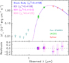 |
Fig. 7. Optical-to-MIR SED of J1813 (open diamonds) from Pan-STARRS1 (teal), UKIDSS (green), and Spitzer (red). The curves represent the best-fit models, an absorbed black body (solid blue line) and three absorbed stellar models from the Kurucz (1993) template library: a B0I model (dotted purple line), B0V model (dashed magenta line), and a B0III model (dot-dashed pink line). The residual (observed minus predicted) fluxes are shown with a small horizontal shift for clarity in the bottom panel (black body: blue circles; B0I: purple diamonds; B0V: magenta triangles; B0III: pink squares). All three models assume an AV = 38 mag. |
The optical-to-MIR spectral energy distribution (SED) of J1813 is extremely red, implying significant obscuration. We fitted the SED with an absorbed black body following Rahoui et al. (2008). The black body model can be parameterized as
 (1)
(1)
where T*, R*, and D* are, respectively, the companion star black body temperature, radius, and distance. The free parameters are T*, R*/D*, and the extinction, AV. We assumed as extinction curve a combination of laws derived for the Galactic plane in different wavelength ranges (Cardelli et al. 1989; Indebetouw et al. 2005; Chiar & Tielens 2006). The best-fit parameters are determined through χ2 minimization after adding a systematic 10% uncertainty to the flux measurements in quadrature. The best-fit black body model and the derived reduced χ2 are displayed in Fig. 7. A single black body yields a good fit with T* = 32 000 ± 4000 K, AV = 38 ± 1, and R*/D* = (3.5 ± 0.5)×10−11. Based on the estimated stellar temperature, the stellar class corresponds to a B star (Payne 1925). The stellar class interpretation is confirmed by the best-fit stellar model obtained after fitting the SED with the Kurucz (1993) stellar library. The best-fit stellar models, also shown in Fig. 7, are given by the class B0I, B0V, and B0III stellar models absorbed by an extinction consistent with that derived from the black body model. Assuming a typical radius of a B0 star (R* ≃ 10 − 20 R⊙; e.g., Coleiro & Chaty 2013), with the lower radius more in line with a main sequence star and the larger radius with a giant, the estimated distance of J1813 would be D* ≃ 6.5 − 13.1 kpc. The derived visual absolute magnitude of J1813 from the black body model ranges from −6.8 to −8.4, depending on the assumed distance, D*. Based on the derived extinction, temperature and luminosity, we conclude that the companion star of J1813 must be an extremely absorbed B star at a distance of 7–13 kpc. An HMXB showing a similar high extinction value is IGR J16320−4751, an O or B supergiant whose compact object is an NS (Lutovinov et al. 2005) and that has an estimated extinction of AV = 35.4 mag (Rahoui et al. 2008). This is quite large compared to the extinction values AV ≲ 20 usually shown by these sources (Pellizza et al. 2006; Rahoui et al. 2008; Torrejón et al. 2010; Coleiro & Chaty 2013; Coleiro et al. 2013; Hare et al. 2019; Fortin et al. 2020; Sidoli et al. 2022).
Assuming the empirical relation between the hydrogen column density and the visual extinction as derived by Foight et al. (2016, i.e., NH (cm−2) = (2.87 ± 0.12)×1021AV), the extinction derived for J1813 corresponds to NH ≃ (1.1 ± 0.1)×1023 cm−2. This column density is slightly lower than the value derived from the X-ray spectrum, which is typical of highly absorbed HMXB systems (e.g., Rahoui et al. 2008). A similar difference is observed in IGR J16320−4751, for which the estimated extinction corresponds to a hydrogen column density NH = 1.0 × 1023 cm−2, lower than that derived from the X-ray spectrum, which is NH ∼ 2.1 × 1023 cm−2.
5. Discussion
We report here on an X-ray transient source showing flaring behavior, which we have identified within EXTraS, analyzing XMM-Newton archival data. During a 100 ks-long observation, the source remained undetected during the initial 60 ks, followed by an active phase with several X-ray flares (lasting a few ks each).
A candidate optical counterpart was found within the X-ray error region. Its SED is consistent with that of a B0 star with a high extinction, implying that J1813 is a new HMXB. From the fit results, we find that any stellar luminosity class is in agreement with the observed SED, although a slightly better fit is obtained with a B0I star. Therefore, the optical counterpart alone (which can be a main sequence, a giant, or a supergiant B star) indicates only a membership within the broad family of HMXBs, but not a secure subtype nature. The optical identification indicates a source located at a distance of ∼10 kpc (between 7 and 13 kpc), allowing us to calculate an average X-ray luminosity of the active phase of about 1035 erg s−1.
The transient nature of the X-ray emission suggests either a BeXRB or an SFXT. The shape of its X-ray light curve, the presence of many short flares, and their temporal and spectral properties strongly favor an SFXT. In particular, the light curve of J1813 is similar to that observed in the archetypal SFXT IGR J17544−2619 with XMM-Newton (Bozzo et al. 2016) and Chandra (in’t Zand 2005): a 150 ks-long XMM-Newton observation caught IGR J17544−2619 in an initial dim X-ray state, followed by a bright X-ray flaring activity lasting 7 ks (Bozzo et al. 2016), very similar to the light curve we have discovered from J1813. A FRED-like profile is observed in the same SFXT, IGR J17544−2619, with Chandra (in’t Zand 2005).
The X-ray luminosity of the active phase in J1813 indicates flaring emission in an intermediate X-ray luminosity, frequently observed in SFXTs (Sidoli et al. 2008; Romano 2015; Sidoli et al. 2019). The amplitude of the observed long-term X-ray flux variability is > 500, measured from the peak of the brightest flare observed by XMM-Newton (no. 8 in Table 2) to the most stringent upper limit reported in Sect. 3.1. The implied X-ray luminosities are in the range from LX < 8 × 1032 erg s−1 to 4 × 1035 erg s−1 (2–12 keV, assuming a distance of 10 kpc), well within typical SFXT flares’ properties (Sidoli et al. 2019). The time-averaged spectrum during the X-ray flaring activity is highly absorbed (NH in excess of 1023 cm−2) and well-fitted by a power-law model (Γ ∼ 1.7), emitting an average luminosity of 7.1 × 1034 erg s−1 (0.2–12 keV). Power-law-like spectra with similar slopes are typical of SFXTs at this level of X-ray emission (Sidoli et al. 2008), while much flatter spectra (Γ ∼ 0.0 − 1.0) are observed only during SFXT outbursts.
The temporal parameters of J1813’s flares (Table 2) match those reported in the investigation of SFXTs observed by XMM-Newton and analyzed within EXTraS (Sidoli et al. 2019). In particular, the waiting time (i.e., the interval of time between two consecutive flare peaks) is in the range 0.69–12.6 ks, in agreement with the waiting time measured in SFXTs (0.15–12.1 ks, with a distribution peaking around 0.4–5 ks). The rise and decay times overlap with the values measured in SFXTs as well. The lack of any known X-ray outbursts (above 1036 erg s−1) in archival X-ray observation of J1813 is also in line with the typical very low duty cycle of SFXTs (less than 5%, but it can be much lower in some members of the class; Sidoli & Paizis 2018).
Regarding the source duty cycle, we estimate that J1813 spends approximately 40% of the time above an X-ray flux of a few 10−13 erg cm−2 s−1 (Sect. 3.1), i.e., above a luminosity of a few 1033 erg s−1. This is in agreement with that measured by Swift-XRT monitoring of a sample of SFXTs (Romano 2015), in particular the sources IGR J08408–4503, XTE J1739–302, and IGR J17544–2619.
On the other hand, if we compare J1813 properties with BeXRBs, short X-ray flares are very rarely observed in this kind of HMXB. And, when present, they happen just before or after the peak of an outburst, with flare peaks much more luminous than those observed in J1813 (Reig et al. 2008). Two anomalous, isolated flares have recently been caught by eRosita (0.2–10 keV) from the BeXRB A0538-66 (Ducci et al. 2022), at orbital phases far from the periastron passage and without concomitant outbursts. However, these flares showed a larger X-ray luminosity (a few 1036 erg s−1) than in J1813 and an unconstrained duration (between 42 s and 29 ks for the first flare and between 29 ks and 57 ks for the second one).
In conclusion, the observed properties of this new HMXB strongly support an identification with an SFXT. However, optical and near-IR spectroscopy are needed to confirm the luminosity class of the donor star and reduce the uncertainty in the source distance.
Project funded by the EU’s FP7 program.
We note that, by using the definition of HR as (ctsH − ctsS)/(ctsH + ctsS), where cts are the photons in the hard (5–12 keV) and soft band (2–5 keV) for a given time bin, we obtain a consistent result.
Acknowledgments
This research has made use of the VizieR catalog access tool, CDS, Strasbourg Astronomical Observatory, France (DOI: 10.26093cdsvizier). The Pan-STARRS1 Surveys (PS1) and the PS1 public science archive have been made possible through contributions by the Institute for Astronomy, the University of Hawaii, the Pan-STARRS Project Office, the Max-Planck Society and its participating institutes, the Max Planck Institute for Astronomy, Heidelberg and the Max Planck Institute for Extraterrestrial Physics, Garching, The Johns Hopkins University, Durham University, the University of Edinburgh, the Queen’s University Belfast, the Harvard-Smithsonian Center for Astrophysics, the Las Cumbres Observatory Global Telescope Network Incorporated, the National Central University of Taiwan, the Space Telescope Science Institute, the National Aeronautics and Space Administration under Grant No. NNX08AR22G issued through the Planetary Science Division of the NASA Science Mission Directorate, the National Science Foundation Grant No. AST–1238877, the University of Maryland, Eotvos Lorand University (ELTE), the Los Alamos National Laboratory, and the Gordon and Betty Moore Foundation. This work is based in part on data obtained as part of the UKIRT Infrared Deep Sky Survey. This work is based in part on observations made with the Spitzer Space Telescope, which was operated by the Jet Propulsion Laboratory, California Institute of Technology, under a contract with NASA. This research has made use of data obtained from the 4XMM XMM-Newton serendipitous source catalog compiled by the XMM-Newton Survey Science Centre consortium. This research has made use of data obtained from the Chandra Data Archive and the Chandra Source Catalog, both provided by the Chandra X-ray Center (CXC).
References
- Bird, A. J., Bazzano, A., Malizia, A., et al. 2016, ApJS, 223, 15 [Google Scholar]
- Bozzo, E., Falanga, M., & Stella, L. 2008, ApJ, 683, 1031 [Google Scholar]
- Bozzo, E., Bhalerao, V., Pradhan, P., et al. 2016, A&A, 596, A16 [NASA ADS] [CrossRef] [EDP Sciences] [Google Scholar]
- Cardelli, J. A., Clayton, G. C., & Mathis, J. S. 1989, ApJ, 345, 245 [Google Scholar]
- Chambers, K. C., Magnier, E. A., Metcalfe, N., et al. 2016, ArXiv e-prints [arXiv:1612.05560] [Google Scholar]
- Chiar, J. E., & Tielens, A. G. G. M. 2006, ApJ, 637, 774 [NASA ADS] [CrossRef] [Google Scholar]
- Churchwell, E., Babler, B. L., Meade, M. R., et al. 2009, PASP, 121, 213 [Google Scholar]
- Coleiro, A., & Chaty, S. 2013, ApJ, 764, 185 [NASA ADS] [CrossRef] [Google Scholar]
- Coleiro, A., Chaty, S., Zurita Heras, J. A., Rahoui, F., & Tomsick, J. A. 2013, A&A, 560, A108 [NASA ADS] [CrossRef] [EDP Sciences] [Google Scholar]
- De Luca, A., Salvaterra, R., Tiengo, A., et al. 2017, in The X-ray Universe 2017, eds. J. U. Ness, & S. Migliari, 65 [Google Scholar]
- De Luca, A., Stelzer, B., Burgasser, A. J., et al. 2020, A&A, 634, L13 [NASA ADS] [CrossRef] [EDP Sciences] [Google Scholar]
- De Luca, A., Salvaterra, R., Belfiore, A., et al. 2021, A&A, 650, A167 [NASA ADS] [CrossRef] [EDP Sciences] [Google Scholar]
- De Luca, A., Marelli, M., Mereghetti, S., et al. 2022, A&A, 667, L7 [NASA ADS] [CrossRef] [EDP Sciences] [Google Scholar]
- Ducci, L., Mereghetti, S., Santangelo, A., et al. 2022, A&A, 661, A22 [NASA ADS] [CrossRef] [EDP Sciences] [Google Scholar]
- Evans, P. A., Page, K. L., Osborne, J. P., et al. 2020, ApJS, 247, 54 [Google Scholar]
- Evans, I. N., Evans, J. D., Martínez-Galarza, J. R., et al. 2024, ApJS, 274, 22 [NASA ADS] [CrossRef] [Google Scholar]
- Flewelling, H. A., Magnier, E. A., Chambers, K. C., et al. 2020, ApJS, 251, 7 [NASA ADS] [CrossRef] [Google Scholar]
- Foight, D. R., Güver, T., Özel, F., & Slane, P. O. 2016, ApJ, 826, 66 [Google Scholar]
- Fornasini, F., Antoniou, V., & Dubus, G. 2023, Handbook of X-ray and Gamma-ray Astrophysics, 143 [Google Scholar]
- Fortin, F., Chaty, S., & Sander, A. 2020, ApJ, 894, 86 [NASA ADS] [CrossRef] [Google Scholar]
- Fruscione, A., McDowell, J. C., Allen, G. E., et al. 2006, in Observatory Operations: Strategies, Processes, and Systems, eds. D. R. Silva, & R. E. Doxsey, SPIE Conf. Ser., 6270, 62701V [NASA ADS] [CrossRef] [Google Scholar]
- Gabriel, C., Denby, M., Fyfe, D. J., et al. 2004, in Astronomical Data Analysis Software and Systems (ADASS) XIII, eds. F. Ochsenbein, M. G. Allen, & D. Egret, ASP Conf. Ser., 314, 759 [NASA ADS] [Google Scholar]
- Garmire, G. P., Bautz, M. W., Ford, P. G., Nousek, J. A., & Ricker, Jr., G. R. 2003, in X-Ray and Gamma-Ray Telescopes and Instruments for Astronomy, eds. J. E. Truemper, & H. D. Tananbaum, SPIE Conf. Ser., 4851, 28 [NASA ADS] [Google Scholar]
- Gendreau, K. C., Arzoumanian, Z., & Okajima, T. 2012, in Space Telescopes and Instrumentation 2012: Ultraviolet to Gamma Ray, eds. T. Takahashi, S. S. Murray, & J. W. A. den Herder, SPIE Conf. Ser., 8443, 844313 [Google Scholar]
- Gotthelf, E. V., & Halpern, J. P. 2009, ApJ, 700, L158 [CrossRef] [Google Scholar]
- Hare, J., Halpern, J. P., Clavel, M., et al. 2019, ApJ, 878, 15 [NASA ADS] [CrossRef] [Google Scholar]
- Indebetouw, R., Mathis, J. S., Babler, B. L., et al. 2005, ApJ, 619, 931 [NASA ADS] [CrossRef] [Google Scholar]
- in’t Zand, J. J. M. 2005, A&A, 441, L1 [CrossRef] [EDP Sciences] [Google Scholar]
- Kretschmar, P., Fürst, F., Sidoli, L., et al. 2019, New Astron. Rev., 86, 101546 [Google Scholar]
- Krimm, H. A., Holland, S. T., Corbet, R. H. D., et al. 2013, ApJS, 209, 14 [NASA ADS] [CrossRef] [Google Scholar]
- Kurucz, R. L. 1993, VizieR On-line Data Catalog: VI/39 [Google Scholar]
- Lawrence, A., Warren, S. J., Almaini, O., et al. 2007, MNRAS, 379, 1599 [Google Scholar]
- Lutovinov, A., Rodriguez, J., Revnivtsev, M., & Shtykovskiy, P. 2005, A&A, 433, L41 [NASA ADS] [CrossRef] [EDP Sciences] [Google Scholar]
- Marelli, M., Tiengo, A., De Luca, A., et al. 2017, ApJ, 851, L27 [NASA ADS] [CrossRef] [Google Scholar]
- Marelli, M., De Martino, D., Mereghetti, S., et al. 2018, ApJ, 866, 125 [Google Scholar]
- Martínez-Núñez, S., Kretschmar, P., Bozzo, E., et al. 2017, Space Sci. Rev., 212, 59 [Google Scholar]
- Mitsuda, K., Bautz, M., Inoue, H., et al. 2007, PASJ, 59, S1 [NASA ADS] [CrossRef] [Google Scholar]
- Nasa High Energy Astrophysics Science Archive Research Center (Heasarc) 2014, Astrophysics Source Code Library [record ascl:1408.004] [Google Scholar]
- Negueruela, I., Smith, D. M., Reig, P., Chaty, S., & Torrejón, J. M. 2006, in The X-ray Universe 2005, ed. A. Wilson, ESA Special Publication, 604, 165 [NASA ADS] [Google Scholar]
- Ochsenbein, F., Bauer, P., & Marcout, J. 2000, A&AS, 143, 23 [NASA ADS] [CrossRef] [EDP Sciences] [Google Scholar]
- Oh, K., Koss, M., Markwardt, C. B., et al. 2018, ApJS, 235, 4 [Google Scholar]
- Payne, C. H. 1925, PhD thesis, Radcliffe College [Google Scholar]
- Pellizza, L. J., Chaty, S., & Negueruela, I. 2006, A&A, 455, 653 [NASA ADS] [CrossRef] [EDP Sciences] [Google Scholar]
- Rahoui, F., Chaty, S., Lagage, P. O., & Pantin, E. 2008, A&A, 484, 801 [NASA ADS] [CrossRef] [EDP Sciences] [Google Scholar]
- Reig, P. 2011, Ap&SS, 332, 1 [Google Scholar]
- Reig, P., Belloni, T., Israel, G. L., et al. 2008, A&A, 485, 797 [NASA ADS] [CrossRef] [EDP Sciences] [Google Scholar]
- Romano, P. 2015, Journal of High Energy Astrophysics, 7, 126 [Google Scholar]
- Scargle, J. D., Norris, J. P., Jackson, B., & Chiang, J. 2013, ApJ, 764, 167 [Google Scholar]
- Sguera, V., Barlow, E. J., Bird, A. J., et al. 2005, A&A, 444, 221 [NASA ADS] [CrossRef] [EDP Sciences] [Google Scholar]
- Sguera, V., Bazzano, A., Bird, A. J., et al. 2006, ApJ, 646, 452 [NASA ADS] [CrossRef] [Google Scholar]
- Shakura, N. I., Postnov, K. A., Kochetkova, A. Y., & Hjalmarsdotter, L. 2013, Physics Uspekhi, 56, 321 [Google Scholar]
- Shakura, N., Postnov, K., Sidoli, L., & Paizis, A. 2014, MNRAS, 442, 2325 [Google Scholar]
- Sidoli, L., & Paizis, A. 2018, MNRAS, 481, 2779 [NASA ADS] [CrossRef] [Google Scholar]
- Sidoli, L., Romano, P., Mangano, V., et al. 2008, ApJ, 687, 1230 [NASA ADS] [CrossRef] [Google Scholar]
- Sidoli, L., Postnov, K. A., Belfiore, A., et al. 2019, MNRAS, 487, 420 [Google Scholar]
- Sidoli, L., Postnov, K., Oskinova, L., et al. 2021, A&A, 654, A131 [NASA ADS] [CrossRef] [EDP Sciences] [Google Scholar]
- Sidoli, L., Sguera, V., Esposito, P., Oskinova, L., & Polletta, M. 2022, MNRAS, 512, 2929 [NASA ADS] [CrossRef] [Google Scholar]
- Sidoli, L., Ponti, G., Sguera, V., & Esposito, P. 2023, A&A, 671, A150 [NASA ADS] [CrossRef] [EDP Sciences] [Google Scholar]
- Torrejón, J. M., Negueruela, I., Smith, D. M., & Harrison, T. E. 2010, A&A, 510, A61 [NASA ADS] [CrossRef] [EDP Sciences] [Google Scholar]
- Verner, D. A., Ferland, G. J., Korista, K. T., & Yakovlev, D. G. 1996, ApJ, 465, 487 [Google Scholar]
- Webb, N. A., Coriat, M., Traulsen, I., et al. 2020, A&A, 641, A136 [NASA ADS] [CrossRef] [EDP Sciences] [Google Scholar]
- Wilms, J., Allen, A., & McCray, R. 2000, ApJ, 542, 914 [Google Scholar]
All Tables
All Figures
|
Fig. 1. EXTraS light curve of J1813 in the 2–12 keV energy band, 250 s time bin, T0 = 354548500. The dotted red line marks the end of the quiescent phase. |
| In the text | |
|
Fig. 2. XMM-Newton exposure-corrected image of J1813 (2–12 keV energy band, observation 0552790101) in counts ks−1 arcsec−2. Left panel: quiescent state, with T < 354610080; right panel: active state, with T > 354610080. |
| In the text | |
|
Fig. 3. Left panel: cumulative curve of the events taken from the XMM-Newton region around J1813 in the 2–12 keV energy band and the cuts described in Sect. 2 (we note that it is not background subtracted). The red area marks the quiescent state; the blue area marks the possible active, nonflaring “intermediate” state. Right panel: zoom of the EXTraS flux curve, shown in Fig. 1, with only the active part of the curve (T0+61500 s). The blue area is the same as in the left panel. |
| In the text | |
|
Fig. 4. Active part of the XMM-Newton EXTraS flux curve (from T0+61500 s), as in Fig. 3, right panel. Upper panel: flux curve (in black) plus the best-fitted model described in Sect. 3.1 (in red), which is composed of a series of ten different flares (in blue). Lower panel: residual curve of the model reported in the upper panel. |
| In the text | |
|
Fig. 5. Chandra flux curves taken in the 2–10 keV energy range. The count rate was converted into 2–12 keV flux using the best-fitted spectrum (see Sect. 3.2). Left panel: observation 6685, 1 ks time bin, and T0 = 274669518; central panel: observation 17440, 2 ks time bin, and T0 = 581548320; right panel: observation 17695, 1 ks time bin, and T0 = 580947681. |
| In the text | |
|
Fig. 6. Total spectrum of J1813. The black and red points are from MOS1 and MOS2 of XMM-Newton obs. 0552790101, respectively, while the green ones are from the Chandra obs. 6685. We also report the best-fitted model, as described in Sect. 3.2. |
| In the text | |
|
Fig. 7. Optical-to-MIR SED of J1813 (open diamonds) from Pan-STARRS1 (teal), UKIDSS (green), and Spitzer (red). The curves represent the best-fit models, an absorbed black body (solid blue line) and three absorbed stellar models from the Kurucz (1993) template library: a B0I model (dotted purple line), B0V model (dashed magenta line), and a B0III model (dot-dashed pink line). The residual (observed minus predicted) fluxes are shown with a small horizontal shift for clarity in the bottom panel (black body: blue circles; B0I: purple diamonds; B0V: magenta triangles; B0III: pink squares). All three models assume an AV = 38 mag. |
| In the text | |
Current usage metrics show cumulative count of Article Views (full-text article views including HTML views, PDF and ePub downloads, according to the available data) and Abstracts Views on Vision4Press platform.
Data correspond to usage on the plateform after 2015. The current usage metrics is available 48-96 hours after online publication and is updated daily on week days.
Initial download of the metrics may take a while.