| Issue |
A&A
Volume 697, May 2025
|
|
|---|---|---|
| Article Number | A117 | |
| Number of page(s) | 19 | |
| Section | Astronomical instrumentation | |
| DOI | https://doi.org/10.1051/0004-6361/202453528 | |
| Published online | 13 May 2025 | |
Enhancing Compton telescope imaging with maximum a posteriori estimation
A modified Richardson–Lucy algorithm for the Compton Spectrometer and Imager
1
Julius-Maximilians-Universität Würzburg, Fakultät für Physik und Astronomie, Institut für Theoretische Physik und Astrophysik, Lehrstuhl für Astronomie, Emil-Fischer-Str. 31, 97074 Würzburg, Germany
2
RIKEN Nishina Center, 2-1 Hirosawa, Wako, Saitama 351-0198, Japan
3
Department of Astronomy, University of Maryland, College Park, MD 20742, USA
4
NASA Goddard Space Flight Center, 8800 Greenbelt Road, Greenbelt, MD 20771, USA
5
Institut für Physik & Exzellenzcluster PRISMA+, Johannes Gutenberg-Universität Mainz, 55099 Mainz, Germany
6
Department of Physics and Astronomy, Clemson University, Clemson, SC 29634, USA
7
Department of Astronomy & Astrophysics, UC San Diego, 9500 Gilman Drive, La Jolla, CA 92093, USA
8
Institute of Astronomy, National Tsing Hua University, Guangfu Rd., Hsinchu City 300044, Taiwan
9
Space Sciences Laboratory, UC Berkeley, University of California, 7 Gauss Way, Berkeley, CA 94720, USA
10
Kavli Institute for the Physics and Mathematics of the Universe (WPI), The University of Tokyo Institutes for Advanced Study, The University of Tokyo, 5-1-5 Kashiwa-no-ha, Kashiwa, Chiba 277-8583, Japan
11
The George Washington University, Department of Physics, 725 21st St NW, Washington, DC 20052, USA
12
Louisiana State University, BatonRouge, LA 70803, USA
13
Kobayashi-Masukawa Institute, Nagoya University, Furo-cho, Chikusa-ku, Nagoya, Aichi 4648602, Japan
⋆ Corresponding author: This email address is being protected from spambots. You need JavaScript enabled to view it.
Received:
19
December
2024
Accepted:
31
March
2025
Abstract
We present a modified Richardson-Lucy (RL) algorithm tailored for image reconstruction in MeV gamma-ray observations, focusing on its application to the upcoming Compton Spectrometer and Imager (COSI) mission. Our method addresses key challenges in MeV gamma-ray astronomy by incorporating Bayesian priors for sparseness and smoothness while optimizing background components simultaneously. We introduce a novel sparsity term suitable for Poisson-sampled data in addition to a smoothness prior, allowing for flexible reconstruction of both point sources and extended emission. The performance of the algorithm is evaluated using simulated three-month COSI observations of gamma-ray lines of 44Ti (1.157 MeV), 26Al (1.809 MeV), and positron annihilation (0.511 MeV), respectively, representing various spatial features. Our results demonstrate significant improvements over conventional RL methods, particularly in suppressing artificial structures in point source reconstructions and retaining diffuse spatial structures. This work represents an important step toward establishing a robust data analysis for studying nucleosynthesis, positron annihilation, and other high-energy phenomena in our Galaxy.
Key words: techniques: image processing / ISM: general / gamma rays: ISM / infrared: diffuse background
© The Authors 2025
 Open Access article, published by EDP Sciences, under the terms of the Creative Commons Attribution License (https://creativecommons.org/licenses/by/4.0), which permits unrestricted use, distribution, and reproduction in any medium, provided the original work is properly cited.
This article is published in open access under the Subscribe to Open model. This email address is being protected from spambots. You need JavaScript enabled to view it. to support open access publication.
1 Introduction
Observations of gamma-ray lines, such as nuclear lines from radioisotopes and the 0.511 MeV line from positron-electron annihilation, are crucial for understanding the origin of elements in our Universe. Gamma-ray line observations were pioneered by balloon experiments in the 1960s and 1970s (for example, Haymes et al. 1969), and our understanding has since deepened through successful satellite missions covering the MeV energy bands, such as CGRO/OSSE (Johnson et al. 1993), COMPTEL (Schoenfelder et al. 1993) and INTEGRAL/SPI (Vedrenne et al. 2003). These missions have uncovered the distribution of gamma-ray lines across our Galaxy, including the diffuse 0.511 MeV emission from the Galactic disk and bulge (for example, Purcell et al. 1997; Knödlseder et al. 2005) and the distribution of 26Al along the Galactic plane (Oberlack et al. 1996; Knödlseder et al. 1999; Bouchet et al. 2015; Siegert et al. 2023). Building upon these achievements, the upcoming Compton Spectrometer and Imager (COSI) satellite is scheduled for launch in 2027 (Tomsick et al. 2023). With a stacked array of germanium cross-strip detectors, COSI is expected to improve gamma-ray line sensitivity by up to an order of magnitude after two years of operation. The primary science objectives of COSI include mapping the spatial distribution of positron annihilation gamma rays and observing nuclear gamma rays from radioactive nuclei.
One of the key techniques to achieve the above science goals is reconstructing an all-sky image from Compton scattering events detected by the instrument. COSI employs a Compton telescope (Kamae et al. 1987) and measures Compton scattering events with its position sensitive detectors. After event reconstruction (for example, Boggs & Jean 2000; Oberlack et al. 2000; Kurfess et al. 2000; Zoglauer et al. 2007; Zoglauer & Boggs 2007; Takashima et al. 2022; Yoneda et al. 2023), an event in a Compton telescope is characterized by a Compton scattering angle and a scattered gamma-ray direction. Then, the incoming gamma-ray direction is constrained to a ring in the sky rather than being uniquely determined as a point (von Ballmoos et al. 1989). Consequently, a statistical method is essential to recover the gamma-ray source distribution from the reconstructed Compton scattering events. Such a method must be capable of solving this inverse and ill-posed problem inherent in Compton telescope data analysis.
Traditionally, the Richardson–Lucy (RL) algorithm has been used for image reconstruction in this field (Richardson 1972; Lucy 1992; Wilderman et al. 1998). It optimizes the flux on each pixel by iteratively maximizing the surrogate function for the log-likelihood, based on the Expectation–Maximization (EM) algorithm (Bishop 2006). It is widely recognized that the conventional RL algorithm enhances locally bright structures by amplifying statistical fluctuations (Allain & Roques 2006). While several modified algorithms, often based on ad-hoc methods, have been proposed to mitigate this issue (for example, Green 1990; Wang & Gindi 1997; Strong 2003; Knödlseder et al. 2005), recent advancements have shown that incorporating various regularization terms within a Bayesian framework can yield more plausible images, that is, less artifact-prone (Ikeda et al. 2014; Morii et al. 2019; Friot-Giroux et al. 2022; Sakai et al. 2023; Morii et al. 2024). As an example of image reconstruction in astronomy, a Bayesian approach has also succeeded in other fields, such as the radio imaging of a black hole shadow (The Event Horizon Telescope Collaboration 2019). Another notable example is NIFTY (Selig et al. 2013), which provides a framework for signal inference problems based on information field theory (Enßlin et al. 2009). NIFTY supports Bayesian inference methods and has been successful in the image analysis of various astronomical data, such as radio (Junklewitz et al. 2016), and GeV gamma-ray observations (Selig et al. 2015).
Despite these advancements, applying such methods to image reconstruction presents unique challenges in MeV gamma-ray astronomy. One significant issue is that L1 norm regularization (Tibshirani 1996) becomes ineffective while it is broadly used for image sparsity in different fields (Ikeda et al. 2014). It is the sum of absolute values of model parameters and promotes sparsity in them, namely, tending to make many parameters exactly zero. Different from other imaging domains, gamma-ray data follows Poisson statistics, and the reconstructed flux in each pixel is strongly tied to the probability maps of incoming photons. Given that the sum of probability is conserved as 1, the L1 norm becomes almost constant (especially when the exposure throughout the sky is uniform as it will be for COSI), rendering it ineffective as a sparsity term. Another critical challenge is that instrumental background events dominate signals. Satellites such as COSI suffer from significant background originating from activation of the spacecraft material caused by charged particles in orbit (for example Weidenspointner et al. 2001; Schönfelder 2004; Hitomi Collaboration 2018; Odaka et al. 2018; Diehl et al. 2018; Cumani et al. 2019). This results in signal-to-background ratios as low as 10% or even much lower. Thus, it is necessary to carefully consider the background and optimize both signal and background simultaneously.
In this paper, we introduce a modified RL algorithm tailored for COSI, addressing the above challenges. The proposed algorithm finds an approximate solution for the maximum a posteriori estimation incorporating regularization terms within the Bayesian framework. In Section 2, we briefly overview the COSI mission. Then, in Section 3, we incorporate a novel sparsity term suitable for Poisson data, as introduced by Ikeda et al. (2014), while simultaneously optimizing background normalization under a gamma distribution. Our framework allows for the flexible introduction of various regularization terms, including inter-pixel correlations (smoothness), and employs a simple method to compute the RL algorithm. To demonstrate the proposed algorithm, we apply it to simulated COSI observation data spanning three months, presenting results for several science cases where sparsity, smoothness, or both are expected to play crucial roles: 44Ti (only point sources expected at 1.157 MeV), 26Al (mostly diffuse extended emission with possible point sources, 1.809 MeV), and positron annihilation (so far only diffuse emission detected with possible point sources within the sensitivity range of COSI, 0.511 MeV). We explain the simulation setup in Section 4, and show the results in Section 5. Through these applications to actual science cases, we illustrate the potential of our method to enhance image reconstruction in MeV gamma-ray astronomy. Finally, we discuss further improvements for the actual data analysis in the future in Section 6.
2 The Compton Spectrometer and Imager
2.1 Overview of the COSI mission
COSI is an upcoming NASA Small Explorer satellite mission planned for launch in 2027 (Tomsick et al. 2023). Based on successful balloon observations (Lowell et al. 2017; Kierans et al. 2020; Siegert et al. 2020; Beechert et al. 2022b; Karwin et al. 2023; Roberts et al. 2025), COSI is designed to survey the entire sky in the energy range of 0.2–5 MeV and study energetic astronomical phenomena through imaging, spectroscopy, and polarimetry. It has four primary science goals: (1) to uncover the origin of Galactic positrons; (2) to reveal Galactic element formation; (3) to gain insight into extreme environments with polarization; and (4) to probe the physics of multimessenger events. The first two objectives, in particular, focus on gamma-ray lines to image our Galaxy at specific energies.
To achieve these science goals, COSI employs a Compton telescope with excellent energy resolution. The core of the COSI instrument consists of an array of 16 high-purity germanium detectors (Tomsick et al. 2023, Figure 1). Each is a double-sided strip detector with 64 strips per side with a strip pitch of 1.162 mm. The detector dimensions are 8 × 8 × 1.5 cm3, and they are arranged in four stacks of four detectors. They are cooled down to 80–90 K with a mechanical cryocooler. The x and y positions of gamma-ray interactions are determined by the strip readouts, while the z positions are measured by the time difference between anode and cathode signals. This configuration acts as a Compton telescope, measuring deposited energies and positions of incident gamma rays via multiple Compton scattering. The five sides of the Compton telescope are surrounded by bismuth germanium oxide (BGO) scintillators, which act as active anticoincidence shields and reduce background events in the satellite orbit.
With this detector design, COSI can instantaneously cover >25% of the sky with a spectral resolution of 6.0 keV at 0.511 MeV and 9.0 keV at 1.157 MeV, while the angular resolution will be 4.1° at 0.511 MeV and 2.1° at 1.809 MeV. COSI is expected to improve the gamma-ray line sensitivity by about one order of magnitude across its energy range during two years of operation.
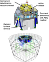 |
Fig. 1 COSI payload design (top) and a schematic of the mass model used in our simulation (bottom). |
2.2 Data structure of COSI observations
Here, we outline the data structure of COSI for scientific analysis, including the image reconstruction (Zoglauer et al. 2021). First, the raw detector output undergoes calibration to produce a list of detected energies and hit positions for each event (Sleator et al. 2019; Beechert et al. 2022a). Then, the path of the scattered gamma ray within the detector is determined using Compton scattering kinematics. Finally, the reconstructed events are compiled into an event list, described by the Compton scattering angle (ϕ), the direction of the scattered gamma-ray (ψ, χ), and the measured gamma-ray energy (Em). We refer to the data space described by these parameters as the Compton Data Space (CDS). Figure 2 shows a schematic of the first three parameters in the CDS. We note that Em is generally different from the incident gamma-ray energy due to detector energy resolution, Compton event misreconstruction, and missing Compton interactions. Most astrophysical analyses, including those described in this paper, typically begin with this processed data since it contains essential information about celestial source signals.
To apply the RL algorithm for image reconstruction, we first create a binned histogram (Di) from the event list in the CDS1. Here, we denote the bin index in this space as i, representing a specific bin in the CDS, and Di is unitless. Our goal is to estimate a model that best describes this data. In the context of all-sky image reconstruction, this model represents the gamma-ray flux in each pixel of the sky, denoted as λj. Here, j is the bin index in the model space, which includes both spatial pixels and an energy axis (Ei), where Ei represents the true initial gamma-ray energy. In the cases of this paper, λj has a unit of cm−2 s−1 sr−1 with a single energy bin because we focus on the gamma-ray lines in our demonstration. We note that generally, the energy axis can have multiple bins, and λj can also represent a differential flux by using its corresponding unit, for example, cm−2 s−1 sr−1 keV−1. Furthermore, we introduce background models, Bik, which we refer to as the background template matrix. This matrix describes the event distribution pattern in the CDS for a certain background component, including instrumental backgrounds such as in-orbit activation. The index k is a label for each background component. The background template matrix does not account for the absolute normalization; thus, we introduce the background normalization bk for each component. Finally, we define a response matrix, Ri j, which connects the model (λ j) to the observed data (Di), essentially describing how a gamma-ray photon from a certain model space bin produces events in the CDS. We explain how we generated these histograms for our numerical tests in Section 4.
With this representation, each iteration of the conventional RL algorithm can be described mathematically as follows:
 (1)
(1)
 (2)
(2)
 (3)
where ϵi is an expected count at the bin index i in the CDS. We note that “old” and “new” indices refer to values before and after an iteration process of the RL algorithm. Through sufficient iterations of this process, the RL algorithm maximizes the log-likelihood defined as
(3)
where ϵi is an expected count at the bin index i in the CDS. We note that “old” and “new” indices refer to values before and after an iteration process of the RL algorithm. Through sufficient iterations of this process, the RL algorithm maximizes the log-likelihood defined as
 (4)
(4)
We note that the bold letters represent the set of parameters, such as λ = {λ1, λ2, ···} and b = {b1, b2, ···}.
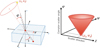 |
Fig. 2 Schematic of Compton Data Space (Kierans 2018). The left panel shows a photon scattering in a detector with the scattering angle ϕ and the scattered gamma-ray direction (ψ, χ). The source position (ψ0, χ0) and photon interaction points are shown. Photons from this source make a cone with a 90° opening angle in the CDS, as shown on the right panel. The apex of the cone corresponds to the source location. |
3 Modified RL algorithm
This section presents a modified RL algorithm tailored for the COSI data analysis2. Our approach introduces prior distributions to solve the image reconstruction as the maximum a posteriori estimation within a Bayesian framework. This modification addresses several challenges for COSI and MeV gamma-ray observations: the ineffectiveness of L1 norm regularization, flexible incorporation of pixel-to-pixel correlations such as Total Square Variation (TSV, Rudin et al. 1992; Chambolle 2004), and simultaneous background optimization.
First, we introduce Bayesian prior distributions Ps(λ) and Pb(b) for the image we want to reconstruct and the normalizations of the background models, respectively. In the framework of the maximum a posteriori estimation, the optimal solution can be defined as the set of parameters (λ, b) that maximizes the following log-posterior probability:
 (5)
(5)
Then, using the EM algorithm, we can derive the solution iteratively. While the E-step remains the same as Equation (1), the M-step is modified such that it finds (λnew, bnew) that maximizes the following function:
 (6)
(6)
The derivation of the above equation is described in Section 3 of Wang & Gindi (1997). In the following subsections, we explain how to derive λnew and bnew separately while introducing the actual formulas for the prior distributions.
3.1 Source
Various methods are proposed to find the parameters that maximize Equation (6) (for example, Morii et al. 2019, 2024). In this paper, we follow the approach of Wang & Gindi (1997). By taking the first derivative of Equation (6) with respect to λnew and setting it to zero, the M-step is modified to solving the following equation:
 (7)
(7)
We note that it is identical to Equation (2) if the prior is constant as typically assumed for the conventional RL algorithm. Generally, solving this equation explicitly is not straightforward for arbitrary prior distributions. In this paper, we separate the prior into a sparse term introduced by Ikeda et al. (2014) and other priors and then solve the above equation approximately.
Ikeda et al. (2014) point out that the L1 norm, commonly used for sparsity in other contexts, is inefficient because the gamma-ray flux corresponds to the probability that a detected gamma-ray originated from a particular pixel and the sum of these probabilities (and also L1) is conserved. As an alternative, they introduced a prior distribution, which can be described in our case as
 (8)
where
(8)
where  is the coefficient for the sparse term. They demonstrated that this prior function can work well as a sparsity term for Poisson-distributed data. This approach has been verified by Morii et al. (2019) using actual X-ray observational data. Given these previous works, we adopt it as our sparsity term. In our case, this prior distribution corresponds to a special case of the gamma distribution with its scale parameter set to infinity as follows:
 (9)
where αs, j and βs, j are shape and scale parameters of the gamma distribution for the flux at pixel j, and Γ(x) is the gamma function.
(9)
where αs, j and βs, j are shape and scale parameters of the gamma distribution for the flux at pixel j, and Γ(x) is the gamma function.
The gamma distribution is the conjugate prior to the Poisson distribution (Bishop 2006), and thus Equation (7) can be solved explicitly if using only this sparsity term (Wang & Gindi 1997). With this feature, we first solve Equation (7) by ignoring other priors and then calculate a correction term. By separating the prior distribution into the sparse term and other priors, we can express it as follows:
 (10)
where fp(λ) is the log probability of the other priors, such as the smoothness prior (TVS), which is introduced in Section 5.2. Then, Equation (7) is expanded as
(10)
where fp(λ) is the log probability of the other priors, such as the smoothness prior (TVS), which is introduced in Section 5.2. Then, Equation (7) is expanded as
 (11)
(11)
To solve the above, we adopt a perturbation approach: we solve the equation by ignoring the last term and derive a correction term afterward. Let  be the solution when the last term is absent (see Ikeda et al. 2014). Then, we introduce the correction term Δωj and describe the solution of Equation (7) as
 (12)
where
(12)
where
 (13)
(13)
In the first-order approximation, the correction term can be determined from the following equation:
 (14)
(14)
Since Equation (14) includes a Hessian matrix, it requires resolving a multidimensional simultaneous system of equations, which is computationally expensive. Thus, we neglect the Hessian term to simplify the solution process and reduce computational cost. This simplification finally leads us to the following equation:
 (15)
(15)
Given that the second term in Equation (14) should be negligible compared to the first term, our solution can be valid when the following condition is satisfied:
 (16)
(16)
This condition does not pose significant problems in most cases relevant to this paper. More details of this point are discussed in Appendix A.
3.2 Background
Similar to the approach we took for the source distribution, the normalization for each background component can be obtained by solving the following equation:
 (17)
(17)
We assume that the prior knowledge for the background normalizations is informed by initial values and associated uncertainties derived by preliminary background modeling. To incorporate this information while solving the above equation explicitly, we again introduce the following gamma distribution as the prior distribution:
 (18)
where αb,k and βb,k are the shape and scale parameters for each background component k. These parameters can be determined from the preliminary background estimation results, considering that its mean and variance are αb,k βb,k and
(18)
where αb,k and βb,k are the shape and scale parameters for each background component k. These parameters can be determined from the preliminary background estimation results, considering that its mean and variance are αb,k βb,k and  , respectively (Bishop 2006). For example, if the background normalization is derived as 1 with a 1% accuracy as 1 σ level, we can set αb,k and βb,k as 104 and 10−4, respectively. On the other hand, we can use (αb,k, βb,k) = (1, ∞) to use a flat distribution when we do not have such prior information. Since the gamma distribution is the conjugate prior to the Poisson distribution, Equation (17) can be solved explicitly as
 (19)
(19)
3.3 Summary of the proposed algorithm
Summarizing the above, we update the source distribution and background normalization simultaneously for each iteration as follows. First, we calculate the expected counts in the CDS as shown in Equation (1). Then, for the source distribution, we calculate the intermediate solution as Equation (13) and then apply the correction term following Equations (12) and (15). The background normalization can be updated simply as Equation (19). Then, we can maximize the log-posterior probability log Q(λ, b) iteratively. It continues until a certain convergence criterion is satisfied, such as when the increase of the log-posterior probability falls below a threshold, or the maximum number of iterations is reached.
4 Simulation setup for algorithm tests
To evaluate the effectiveness of our proposed algorithm for the upcoming COSI observations, we applied it to simulation data spanning three months. We prepared three datasets with distinct spatial features: 44Ti (point source), 26Al (smooth distribution over the Galactic disk), and e+/e− (combination of sparse and smooth components). These datasets allow us to test different aspects of our algorithm: the sparseness prior (44Ti), the smoothness prior (26Al), and the combination of multiple priors (e+/e−). Additionally, we conducted background simulations assuming the conditions of the COSI satellite orbit and generated a response matrix using large-scale simulations. The following sections provide details on each source model, the background simulations, and the response matrix generation process.
4.1 Source model
For our source simulations, we employed the Medium-Energy Gamma-ray Astronomy library (MEGAlib), a comprehensive software package designed for gamma-ray detectors specializing in Compton telescopes (Zoglauer et al. 2006). Our simulated observations spanned three months, assuming an equatorial orbit at an altitude of 550 km with zenith pointing, considering Earth occultation. After performing the Monte Carlo simulations, we generated a binned histogram in the CDS for each source distribution within the Galactic coordinate system. In the following, we briefly describe the source models for 44Ti, 26Al, and 0.511 MeV emission3.
4.1.1 44Ti
44Ti is primarily produced during the alpha-rich freeze-out phase in the explosion mechanisms of core-collapse supernovae and Type Ia supernovae (Thielemann et al. 1990; Nomoto et al. 2006; Maeda et al. 2010). It has a lifetime of about 85 years, decaying to 44Sc, which subsequently decays to 44Ca with a lifetime of approximately 3.9 hours, producing a gamma-ray line at 1.157 MeV (Ahmad et al. 2006). Due to its relatively short lifetime, 44Ti can be a tracer for young supernova remnants in our Galaxy, typically those with ages up to a few hundred years.
To investigate the behavior of the sparse prior under high background events, we modeled the 44Ti distribution as a point source at Cas A (Grefenstette et al. 2014). Gamma-ray and X-ray lines from 44Ti were firmly detected by previous observations (Iyudin et al. 1997; Grefenstette et al. 2014; Siegert et al. 2015), and thus Cas A is the primary target for COSI in the early phase of its operation. While the flux of 44Ti is slightly different among the previous results, we adopted the flux from the INTEGRAL/SPI analysis (Siegert et al. 2015), which is 3.5 × 10⁻⁵ ph cm−2 s−1. We note that while this flux is detectable in our simulated three-month observation, the line sensitivity of COSI is expected to improve significantly with longer observation times. For instance, over its planned 2-year mission, COSI will achieve approximately a few ×10−6 ph cm−2 s−1, allowing for studying fainter 44Ti sources.
4.1.2 26Al
26Al is a long-lived radioactive isotope with a lifetime of about 1 Myr, decaying to 26Mg via β+ decay and producing a 1.809 MeV gamma-ray line (Norris et al. 1983). It is generated and injected into our Galaxy through stellar winds and supernova explosions (Diehl et al. 2006). COMPTEL provided the first flux map of 26Al emission across the Galactic plane (Diehl et al. 1995). While localized hotspots may exist, the overall 26Al distribution is relatively smooth over the Galactic plane due to its long lifetime, tracing the cumulative effects of stellar nucleosynthesis and Galactic chemical evolution over timescales ≳1 Myr.
For the algorithm test, we modeled 26Al as a smooth spatial distribution. It is represented as a doubly exponential disk model in our Galaxy as a three-dimensional model, given by
 where L is the total luminosity of 26Al in our Galaxy, that is,
  , with m = 26u the atomic mass of 26Al nuclei, p = 0.9976 the branching ratio to emit a photon, and τ = 1.05 Myr the lifetime of 26Al. This gives a quasi-persistent luminosity for a living 26Al mass M. The values Rs and zs are the scale radius and scale height, respectively. The radial coordinate is given by
  , and z is the vertical coordinate, z = z′ − z0, where x0 = 8.178, y0 = 0, and z0 = −0.019 are the coordinates of the Galactic center seen from Earth. All distance and size units are in kpc. The line of sight integration was performed so that the flux per pixel with 3 deg resolution is in units of ph/cm2/s/sr. We adopted M = 6 M⊙, Rs = 5.0, and zs = 1.0, which results in a total flux of 1.8 × 10⁻³ ph/cm2/s, compatible with previous observations (for example, Pleintinger et al. 2023).
4.1.3 e+/e−
The 0.511 MeV gamma-ray line, produced by the annihilation of positrons with electrons, has been detected by various missions over five decades (see Siegert 2023, for review). Despite extensive observations, including recent balloon observations (Kierans et al. 2020; Siegert et al. 2020), the origin of these positrons remains unclear. However, it is known that positron annihilation occurs prominently close to the Galactic center region, with a flux comparable to that of the Galactic disk 0.511 MeV emission. While the exact spatial distribution of the 0.511 MeV emission is still under investigation, several models have been proposed. For our simulation, we implemented two different models derived from INTEGRAL/SPI analysis: Skinner et al. (2015) and Siegert et al. (2016).
Skinner et al. (2015) propose a model consisting of a point source at the Galactic center, two Gaussian components for the Galactic bulge emission slightly offset from the center, and a Galactic disk emission with a scale height of 3 degrees, explains the SPI data the best. In contrast, Siegert et al. (2016) claims that the Galactic disk has a larger scale height of 10.5 degrees vertically and a longitudinal extent of 60 degrees. We refer to the former and latter as the thin and thick disk models, respectively. The two different spatial distributions were derived from different data treatments. This originated because it is challenging to distinguish a spatially broad feature from the instrumental backgrounds with the coded aperture mask instruments adopted by SPI. Since these models have several spatial components featuring both sparse and smooth characteristics, we used them as test cases to evaluate the performance of the proposed algorithm. We summarized the parameters for these 0.511 MeV spatial models in Table 1. Additionally, based on Siegert et al. (2016), the line shape of 0.511 MeV emission was assumed to be a Gaussian with FWHM of 2 keV and 3 keV for the bulge and disk components, respectively. We note that the intrinsic line width was ignored for the 44Ti and 26Al cases.
Spatial distribution model parameters for the 0.511 MeV emission.
4.2 Background simulations
For the background simulations, we employed MEGAlib to simulate three months of instrumental and astrophysical backgrounds, assuming the same orbit as the source simulations. The background components included albedo emission, extragalactic gamma-ray background, and instrumental backgrounds caused by cosmic rays bombarding the instrument. The instrumental backgrounds, which have both prompt and delayed components, are mainly due to primary protons, primary alpha particles, atmospheric neutrons, primary electrons, primary positrons, and secondary protons. The input spectra were based on the model from Cumani et al. (2019), with considering the changing geomagnetic cutoff along the orbit. We note that charged particles trapped in the South Atlantic Anomaly (SAA) were not included in our current simulations4.
After simulations, we produced a binned histogram by adding all components, applied Gaussian smoothing on the ψχ plane in the CDS to mitigate the Poisson fluctuation in the background model, and created the total background model in the CDS histogram. Background events were then re-sampled in the CDS according to the Poisson distribution to simulate data. For simplicity in this study, we assumed a single background component, and the proposed algorithm optimized its normalization parameter. In this paper, we focus on evaluating the performance of the RL algorithm under this idealized condition, while background modeling typically involves multiple components and potential model uncertainties in real observations. Addressing these complexities is beyond the scope of the current study, but the optimization of multiple background components and the handling of model uncertainties could potentially lead to further refinements in our data analysis. We discuss these aspects in more detail in Section 6. The number of extracted events for source and background of each target is shown in Table 2.
In our implementation, the background is modeled in the CDS. While some astrophysical backgrounds, such as extragalactic gamma-ray background, could theoretically be modeled in the model space through the response matrix Rij similar to source components, we choose to incorporate all backgrounds as the background template matrix Bik for algorithmic consistency. This approach simplifies the implementation by treating all non-source events uniformly and also conceptually separates the signal of interest from all other contributions. In principle, an astrophysical background component that is initially representable through Rij can be converted into the Bik representation by pre-convolving it with the response. Therefore, from the algorithm’s perspective, the distinction between different background types is not necessary, and all background events are treated equivalently as matrices in the CDS.
Number of events filled in a histogram for the three-month simulation of each source distribution.
4.3 Response matrix generation
The response matrix for our analysis was generated using largescale simulations with MEGAlib. We simulated more than 1012 events uniformly distributed over 4π steradians with the same initial gamma-ray energy as each source distribution and created a response matrix in the detector coordinates. Then, we integrated the response matrix over time while weighting it with the time-dependent satellite attitude and Earth occultation effects over the three months, and produced the final response matrix in Galactic coordinates. The number of bins for each element in the response matrix is shown in Table 3. The actual numbers of simulated events are also presented in this table. For the Galactic sky and ψχ plane, we used HEALPix pixelization (Górski et al. 2005). Figure 3 shows the effective area convolved with the exposure time for each case. Two regions with relatively short exposure times can be observed, which is because we assumed zenith pointing for simplicity in this simulation. COSI is planned to observe the sky by pointing 22° north, then south, of zenith with approximately a 12-hour period, which will result in a more uniform exposure map.
5 Results
Here, we present the results of applying our algorithm to the three science objectives. We first evaluate the effect of the sparseness term using the 44Ti simulation and then test the smoothness term with 26Al. Finally, we analyze the combined effect of both terms using the 0.511 MeV dataset.
The stopping criterion for the RL algorithm was set to when the increase in the log-posterior probability became less than 10−2. We performed our data analysis on a workstation equipped with an Intel Core i9-10980XE processor and 256 GB memory. To accelerate computational time related to the response matrix, we utilized an NVIDIA A6000 GPU and the CuPy library (Okuta et al. 2017). Typically, we were able to execute about 20 iterations per second. While the total computation time and number of iterations varied depending on the prior distribution parameters, image reconstruction for a single parameter set was computed within 1–3 minutes.
5.1 44Ti: a point source + a sparsity prior
To evaluate the sparse imaging analysis, we set the prior distribution of the source as the following equation:
 (20)
(20)
Here we used the same coefficient cSP for all of the pixels and varied it from 10−4 to 3 × 10⁻¹. For the background model, we initially assumed a flat distribution (αb = 1 and βb = ∞), which results in Equation (19) becoming the conventional RL algorithm for the background part. The effect of the background optimization is discussed later.
5.1.1 Reconstructed image and flux
The reconstructed images are shown in Figure 4. As cSP increased, the diffuse structure around point sources was gradually suppressed. We saw that, at cSP ≈ 2 × 10⁻¹, the diffuse structure around point sources disappeared completely. At this point, only the point source remained at the location of the injected source. When cSP was increased more, the image flux finally became zero. We investigated this feature more by plotting the sparse term against the log-likelihood, as shown in Figure 5. The log-likelihood initially increased from cSP = 10−4 to cSP = 10−2 as the diffuse structure around the point source was suppressed. Then, above cSP ≈ 10−2, the log-likelihood began to drop. It reached some local minima, for instance, around cSP = 10−1. As cSP was increased, point-source artifacts disappeared, as seen from cSP = 3 × 10⁻² to cSP = 1 × 10⁻¹ in Figure 4. The discrete change in the image corresponded to the local minimum observed in the log-likelihood curve. We also show the log-likelihood and log-posterior distribution values for each iteration at cSP = 10−2 in Figure 7. This plot indicates that the algorithm optimized the log-likelihood and then maximized the sparse term.
Figure 8 shows the reconstructed flux depending on different cSP. Here, the reconstructed flux of the source is defined as the sum of flux values in a pixel at the source location and its adjacent 8 pixels. In this case, the source flux was reconstructed within 3–10%, depending on cSP. Furthermore, we show the reconstructed flux outside the source, which should be ideally zero but was bound to be positive due to the Poisson fluctuations (Figure 9). With increasing cSP, the flux outside the source became smaller, and finally almost zero after cSP ∼ 10−1. Notably, the flux outside the source was not negligible when cSP was small. It could be a few ×10−5 ph cm−2 s−1, which is of the same order as the injected source flux. In this case, the Poisson fluctuation of the background events (∼103) was comparable to the number of photon events collected from the source (see Table 2). Then, the conventional RL algorithm assigned some of the fluctuations to gamma-ray emission, which led to a significant flux outside the source location. With a time-integrated effective area of about 108 cm2 s, the background caused an uncertainty of O(10−5) ph cm−2 s−1. Introducing the sparseness prior can mitigate such a problem by suppressing the artifacts, resulting in better flux estimation.
Binning of the response matrix for each target.
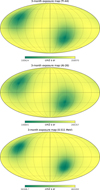 |
Fig. 3 Exposure maps for the three targets with three-month observations in Galactic coordinates. The exposures for 44Ti, 26Al, and 0.511 MeV are shown from top to bottom. The values represent the effective area integrated over both the observation time and the solid angle of each pixel. The solid angle per pixel is 4.1 × 10⁻³ sr, and the number of pixels is 3072. The range of the color bar is different in each case. It should be noted that the color bars of the images shown in this paper are in the log scale. |
5.1.2 L-curve method
It should be noted that determining the optimal cSP is not always straightforward and may depend on various factors, including specific scientific goals, the nature of the dataset, and the particular features of interest in the analysis. While several methods are proposed to determine the optimal prior distribution, here we adopted the L-curve method by following Allain & Roques (2006). In this method, an optimal solution can be derived as the ma0ximum curvature point in a graph between statistics and penalty values, corresponding to Figure 5. We note that the graph in the figure took an inverted L shape since the log-likelihood was plotted on the y-axis. When applying the L-curve method, we normalized both the x-axis and y-axis to have the same range. This method suggested cSP ≈ 10−1 as the optimal value (see Figure 6), but it was likely affected by the sudden change in the L-curve due to several local maximum curvature as seen in Figure 5. Considering the global trend of the L-curve and the maximum value of the likelihood, cSP ≈ 10−2 would also be a candidate for the solution. In this particular case, it would be necessary to determine the optimal solution by combining other methods, such as visual inspection and cross-validation, according to a specific purpose, for example, the flux from a specific region, the flux from the entire region, or the identification of the location of a known point source, etc. We further discuss this point in Section 6.
5.1.3 Background normalization
Here, we investigate the effect of different prior distributions on the background model normalization. In addition to the flat distribution, we used the gamma distribution, assuming a precise determination of the normalization parameter with 0.1% accuracy. Specifically, we set (αb, βb) = (106, 10−6). This value was chosen to be comparable to the Poisson fluctuation of the number of background events.
We added the resulting fluxes from the source and outside its region as the dashed lines in Figures 8 and 9. It can be seen that the flux from the source region was better reconstructed, especially around cSP ≈ 10−2, where the likelihood reached the maximum in both cases. We note that the flux became larger after that, which likely corresponded to overfitting, and then sharply dropped to zero since the sparsity prior became too strong. We also show the optimized background normalization in Figure 10. While the background normalization converged well in both cases, it converged closer to 1 with the 0.1% prior distribution, indicating the strong influence of the prior information on the estimation. Although it might be unlikely that the background normalization is determined within 0.1% accuracy in advance, this approach can, in principle, incorporate such background information, potentially improving the estimation of both the source and background. In real observations, such a constraint on the background would be helpful when the number of detected events is small, such as in transient event analysis. In addition, it may be possible to optimize the background splitting into different components using detector information. We discuss it again in Section 6.
 |
Fig. 4 Reconstructed images of 44Ti with different values for cSP. The left top panel shows the injected model for 44Ti. From the next to bottom right, cSP is set to 10−4, 10−2, 3 × 10⁻², 1 × 10⁻¹, and 2 × 10⁻¹. |
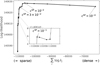 |
Fig. 5 L-curve for the sparse prior. The x-axis shows the sparseness defined as ∑j log λj, while the y-axis shows the resulting log-likelihood. |
 |
Fig. 7 Log-posterior and log-likelihood for each iteration. Here, cSP is set to 10−2. |
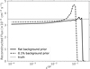 |
Fig. 8 Reconstructed flux compared with the simulated one. The solid line corresponds to using the flat prior distribution for the background normalization, while the dashed line is for the prior distribution with 0.1% accuracy. |
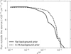 |
Fig. 9 Flux outside the source. |
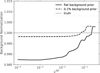 |
Fig. 10 Optimization of the background normalization. |
5.2 26Al: a diffuse emission + a smoothness prior
Next, we evaluate the performance of the algorithm on smooth, extended sources. Here, we applied our method to the simulated 26Al data. For this case, we introduced TSV as a smoothness prior. It is described as follows:
 (21)
where cTSV is the coefficient controlling the strength of the smoothness constraint, and σj represents the set of indices for pixels adjacent to pixel j. We varied cTSV from 104 to 107 to examine its effect on the reconstructed images. The background model was treated the same as in the 44Ti case, assuming a flat distribution.
(21)
where cTSV is the coefficient controlling the strength of the smoothness constraint, and σj represents the set of indices for pixels adjacent to pixel j. We varied cTSV from 104 to 107 to examine its effect on the reconstructed images. The background model was treated the same as in the 44Ti case, assuming a flat distribution.
5.2.1 Reconstructed image
The reconstructed images for various cTSV values are presented in Figure 11. At smaller cTSV values, the images showed more noise and artificial structures. As cTSV increased, the distribution became smoother, more closely resembling the expected extended emission from 26Al. Here, we set the minimum value in the images to 10−4 cm−2 s−1 sr−1 from a rough estimation of the noise level. Assuming the background events affect an image uniformly over the sky, each pixel suffers from ∼70 background events (= 2.26 × 10⁵/3072), which means a Poisson fluctuation of ∼8 events per pixel. Given the typical exposure of 2 × 106 cm2 s sr per pixel, this fluctuation corresponds to ∼10−4 ph cm−2 s−1 sr−1.
Figure 12 shows the relationship between the TSV and the log-likelihood for different values of cTSV. As cTSV increased, we observed a clear trade-off between image smoothness and likelihood optimization. Visual inspection suggested that cTSV ≈ 105−6 provided a good balance between noise suppression and preserving the overall structure of the 26Al distribution. At this value, the large-scale features of the Galactic plane emission were well-recovered, while smaller-scale noise was effectively suppressed. To quantitatively assess the optimal cTSV, we again employed the L-curve method (Allain & Roques 2006). This analysis suggested an optimal value of cTSV = 1.78 × 10⁵ (see Figure 13). In this case, the optimal solution obtained by the L-curve method was consistent with the visual evaluation.
5.2.2 Comparison with the conventional algorithm
Figure 14 compares the input model, the results with the proposed algorithm (cTSV = 1.78 × 10⁵) and the conventional RL algorithm. The conventional approach showed that its solution converged to a distribution composed of numerous point-like structures, enhancing statistical fluctuations in the data. Such a result makes it challenging to discuss the spatial scales and morphology of the diffuse emission that are crucial for 26Al science. In contrast, the proposed algorithm maintained a continuous spatial distribution in its solution. The resulting image allows us to discuss the spatial characteristics of the 26Al emission. For instance, we could see a contour line with a flux of 3 × 10⁻⁴ph/cm2/s/sr and claim that it extends ±∼90 degrees along the Galactic plane. This distribution closely matched the input model whose extension is ± ∼ 100 degrees. We also show the fluxes obtained along the Galactic longitude and latitude for each algorithm in Figure 15. The fluctuations seen in the conventional method were clearly suppressed in the proposed one, and the flux and structure around the Galactic center were well recovered. The total flux was obtained as 1.82 × 10⁻³ cm−2 s−1, which is consistent with the injected model within ∼1%. This demonstrates the effectiveness of our method with the introduced prior in reconstructing extended smooth sources such as 26Al emission.
5.3 e+/e−: multiple spatial components
Finally, we evaluate the performance of our algorithm for the 0.511 MeV emission, which presents a complex scenario combining several spatial components. For this case, we incorporated both the sparseness and smoothness priors as follows:
 (22)
(22)
We varied cTSV from 102 to 106 and cSP from 10−2 to 5 × 10⁻¹ to examine their effects on the reconstructed images.
First, we focus on the thin disk model. This model includes a point source at the Galactic center, two Gaussian components for the Galactic bulge emission slightly offset from the center, and a Galactic disk emission with a scale height of 3 degrees. In Appendix B, we show the reconstructed images for various combinations of cTSV and cSP for the thin disk model. As expected, we observed a smoother distribution over the Galaxy as we increased cTSV. Increasing cSP, on the other hand, suppressed the point-like structures.
Figure 16 shows the relationship between the log-likelihood, TSV, and sparseness terms. We applied the L-curve method two-dimensionally. First, we scanned the curvature along the cTSV axis for each value of cSP. For all values of cSP, we found the maximum curvature at cTSV = 104. Next, we scanned the curvature along the cSP axis while fixing cTSV at 104. Then, we found two local maxima in the curvature of the graph (see Figure 17). Thus, two primary candidates for optimal solutions were identified: (cTSV, cSP) = (104, 3.2 × 10⁻²) and (cTSV, cSP) = (104, 2.2 × 10⁻¹). The red frames in Figure B.1 indicate the two candidates. Upon visually inspecting the reconstructed images, we found that the latter solution resulted in a truncated disk with unnatural structures. Therefore, we selected the former solution of (cTSV, cSP) = (104, 3.2 × 10⁻²) as the most plausible reconstruction for this analysis. We also show the expected counts from the selected model compared with the data in the CDS in Appendix C.
Figure 18 compares the input model, the results from our Bayesian method (using the selected optimal cTSV and cSP values), the conventional RL algorithm, and the RL with a noise damping approach used in Knödlseder et al. (2005); Siegert et al. (2020). In the last case, we adopted a 5-degree Gaussian filter. One of the key advantages of our proposed method is the suppression of artifacts commonly observed in other approaches. The bright artifacts shown in the upper left and lower right regions of the conventional RL and noise-damping RL results were significantly reduced in our method. These artifacts corresponded to regions with shorter exposure times (see Figure 3), where low photon statistics led to enhanced fluctuations in the conventional methods. Our approach successfully mitigated this issue, resulting in a substantial improvement in flux estimation, as also seen in the 44Ti case. Table 4 shows the obtained total fluxes with different methods. While the other methods overestimated the total flux by approximately 60% due to these artifacts, our method achieved an accuracy within 10% of the true value.
Another improvement was that the continuous disk structure was preserved. Traditional methods tend to emphasize point-like structures, as observed in the 26Al case, breaking up the inherently diffuse, connected structure into discrete segments. Our method maintained the continuity of the disk, enabling more discussion of its spatial structure. This would be crucial for analyzing the large-scale distribution of the 0.511 MeV emission in the Galaxy.
It is important to note a potential limitation of our method: the over-smoothing of the Galactic center structure. When examining the flux along Galactic longitude and latitude, as shown in Figure 19, we observed that our reconstruction of the central region was broader than the input model. This over-smoothing likely resulted from applying a uniform smooth prior across the entire sky. While this approach worked well for the disk structure, it might be excessively strong for the brighter, more sharply defined central region. Future improvements could involve varying the strength of the prior based on the region, potentially using adaptive priors that account for the diverse structural characteristics across the Galactic plane. Despite this limitation, the overall performance of the proposed method in reconstructing the 0.511 MeV emission demonstrated a significant advancement over conventional techniques, particularly in suppressing point-like artifacts and preserving extended structures.
We also applied our method to the thick disk model. The results, shown in Figures 20 and 21, demonstrated that our method performed well for this alternative model as well. Our algorithm successfully reconstructed the smooth distribution of the bulge and the thicker disk emission without introducing significant spurious point sources, while the conventional RL again showed a fragmented distribution. The successful application of our method to both the thin disk and thick disk models demonstrates its robustness to different underlying source structures. This case illustrates the power of combining sparseness and smoothness priors in our modified RL algorithm, enabling accurate reconstruction of complex emission scenarios that include both point-like and diffuse components with varying scale heights. These results suggest that three months of COSI observations might be sufficient to discriminate between competing 0.511 MeV emission models, which would advance our understanding of positron annihilation distribution in the Galaxy.
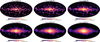 |
Fig. 11 Reconstructed images of 26Al with different values for cTSV. From top left to bottom right, cTSV is set to 104, 105, 3.16 × 10⁵, 106, 3.16 × 10⁶, and 107. The injected model is shown in Figure 14. |
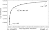 |
Fig. 12 L-curve for the smooth prior. The x-axis shows the total squared variation, while the y-axis shows the resulting log-likelihood. |
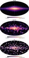 |
Fig. 14 Comparison between the reconstructed images obtained with different methods. The images are in the units of ph/cm2/s/sr. The top shows the injected model for the 26Al map, while the middle and bottom show the reconstructed image with the proposed algorithm and the conventional RL algorithm, respectively. |
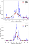 |
Fig. 15 Reconstructed 26Al fluxes along the Galactic longitude (top) and latitude (bottom). |
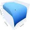 |
Fig. 16 Two-dimensional L-curve for the sparse and smooth priors. The bottom plane corresponds to the smoothness and sparseness, while the z-axis shows the resulting log-likelihood. The black point corresponds to the optimal solution we presented in the main text. |
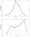 |
Fig. 17 Curvature plots for the two-dimensional L-curve shown in Figure 16. Top: Curvature along cTSV with cSP fixed at its optimal value (3.2 × 10⁻²). Bottom: curvature along cSP with cTSV fixed at its optimal value (104). |
6 Discussion
The results presented in this paper demonstrate the effectiveness of our modified RL algorithm for image reconstruction in COSI observations. Our method successfully combines the sparseness and smoothness priors, enabling accurate reconstruction of complex gamma-ray spatial distributions. While the current implementation shows promising results, we want to discuss several avenues for further improvements and expansion of this approach.
One of the key strengths of our method is its flexibility in incorporating different prior distributions. In this study, we focused on the sparse term introduced by Ikeda et al. (2014) and the TSV for smoothness. While this combination has been demonstrated in Morii et al. (2019) with X-ray data, and solved by EM algorithm and the proximal gradient method (Beck & Teboulle 2009), our framework allows for straightforward extension to any prior distribution if it is first-order differentiable, such as the entropy term and total flux density regularizer. We can explore more sophisticated or physically motivated priors that could further enhance reconstruction quality. Particularly, we found that applying a smooth prior distribution to the entire sky could blur the structure of the 0.511 MeV emission at the Galactic center. As the spatial profile of the Galactic center could help to understand the origin of the 0.511 MeV emission, including some dark matter scenarios (Finkbeiner & Weiner 2007), it is important to address this issue.
Several approaches are possible to make improvements. One is to adopt spatially varying priors. We can vary the coefficient for the prior depending on the location in the sky. Since the central region was well-reconstructed without the smooth prior, weakening the strength of the smooth prior around the Galactic center would mitigate such a problem. Another approach could be to explore edge-preserving smoothness priors that can maintain sharp transitions, as seen in the boundary of the Galactic central region. Allain & Roques (2006) discussed that the total-variation-type regulator could work well when reconstructing sharp edges with INTEGRAL/SPI simulation data of some artificial spatial distributions. It is worth investigating a similar prior (or its combination with other priors) using Compton telescope data, assuming science cases such as those performed in this paper. Finally, we want to mention that the gamma distribution introduced in the background can also be used for the source prior in principle. As discussed in Section 3.1, the sparseness term can be interpreted as a special case of the gamma distribution (see Equation (9)). Even if we use a general gamma distribution, the argument in Section 3.1 holds after a minor modification, namely replacing  with a solution with the general gamma distribution as shown in Equation (19). It would allow us to include prior information about the flux and the flux uncertainty of each pixel if we have them, for example, when we want to incorporate results from previous observations in the data analysis.
While this paper focused on the gamma-ray lines, the proposed method can be applied to other science cases. A promising direction is extending our method to simultaneous spatial-spectral deconvolution. This paper focused on applying the TSV prior only in the spatial domain, but it can be naturally extended to include smoothness constraints in the energy dimension as well. This capability could be particularly effective for analyzing diffuse continuum emission, such as the Galactic diffuse continuum emission (GDCE), where both spatial and spectral distributions are intrinsically smooth. The origin of the GDCE in the MeV band is not yet fully understood, which is sometimes referred to as “COMPTEL excess” or “MeV hump” (for example, Strong et al. 1996; Tsuji et al. 2023; Karwin et al. 2023). The spatial-spectral deconvolution with such smoothness priors could lead to a better determination of the spectral and spatial properties of the GDCE with future COSI data. Moreover, our method can also be applied to transient events such as Gamma-Ray Bursts. In these cases, the sparseness prior could be particularly effective, as demonstrated in the 44Ti analysis with relatively limited statistics. For transient events, where rapid localization is crucial, our algorithm could help to identify point sources by combining the sparseness prior with background constraints.
The basic capability of background optimization was demonstrated within this framework, which is crucial for COSI and MeV gamma-ray observations due to the complex nature of the background. While our demonstration was a simple case, we can refine this approach by optimizing several background components separately in future actual data analysis. For instance, we can assign a single normalization factor to astronomical backgrounds, such as the extragalactic background, for the entire observation period. Simultaneously, we can prepare independent normalization factors for different time segments to account for time-variable instrumental background (Siegert et al. 2019). This multicomponent approach could further improve the accuracy of source reconstruction. The main germanium detectors of COSI are surrounded by BGO active shields. Additionally, the instruments of COSI include the Background Transient Monitor, which is a set of four NaI detectors (Gulick et al. 2024). The data from these instruments, such as the count rates of saturated events and the light curves from the BGO above 2 MeV, can serve as a tracer of the charged particle flux and provide valuable information for determining the background normalization. Integrating these data into our algorithm could further improve the accuracy of background estimation in the future.
When applying this method to real COSI observation data, computational efficiency is also a factor to be considered. While our current implementation achieved reasonable computation times for the 3.7-degree resolution used in this study, we may need to use finer spatial resolution in the model and data space to discuss more detailed spatial structure. Such a finer resolution would be required to analyze the Galactic central region of the 0.511 MeV emission and to conduct point source studies as demonstrated in the 44Ti case. This can significantly increase the computational demands due to the larger data size of the response matrix, which might require handling a large response matrix with a size of O(100) GByte. In future applications, we can explore parallel computing using supercomputers, acceleration using GPU clusters, and further algorithm optimization. In addition, acceleration techniques for the RL algorithm, such as SQUAREM (Du & Varadhan 2020), can improve the computational speed.
Finally, optimizing prior parameters is crucial when applying this method to real observational data. The L-curve method worked to some extent in our demonstrations, but we needed to rely on visual evaluation in some cases, which caused ambiguity in determining an optimal solution. For longer observation times, data-driven methods such as cross-validation could be an alternative. For example, Morii et al. (2019, 2024) used k-fold cross-validation and showed that it worked successfully for their X-ray image analysis. Such a technique could potentially be viable for future data analysis.
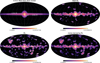 |
Fig. 18 Comparison between the reconstructed 0.511 MeV images with different methods. The images are in the unit of ph/cm2/s/sr. The top left shows the injected thin model, while the reconstructed images with the proposed method, the conventional RL, and the RL using a Gaussian filter are shown on the top right, bottom left, and bottom right panels, respectively. Following the same discussion in Section 5.2.1, each pixel suffers from the Poisson fluctuation of ∼1000 background events (= 2.09 × 10⁶/3072) with a typical exposure of 3.5 × 105 cm2 s sr on a pixel, which corresponds to a noise level of ∼10−4 ph cm−2 s−1 sr−1 in the reconstructed image. |
Total fluxes of the reconstructed 0.511 MeV images with different algorithms.
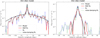 |
Fig. 19 Reconstructed 0.511 MeV fluxes along the Galactic longitude (left) and latitude (right). When plotting the model line, the flux from the point source in Table 1 is blurred with the pixel size of the image (∼3.7 degrees). |
7 Conclusions
In this paper, we presented a modified RL algorithm tailored for image reconstruction in Compton telescope observations, especially focusing on the upcoming COSI mission. Our method addressed key challenges in MeV gamma-ray astronomy by incorporating Bayesian priors for sparseness and smoothness within a maximum a posteriori framework while simultaneously optimizing background components.
Through the above simulations of 44Ti, 26Al, and e+/e−, we demonstrated the effectiveness of our approach in reconstructing both point sources and extended emissions. The sparseness prior effectively suppressed artificial structures in point source reconstructions, while the TSV prior significantly improved the reconstruction of extended sources. The combination of these priors allows for accurate reconstruction of complex emission scenarios, such as the 0.511 MeV sky, where both point-like and diffuse components are present. Our demonstration showed that different spatial models of 0.511 MeV emission can be distinguished even with a three-month early phase of COSI operation.
These results suggest that our modified RL algorithm could improve image reconstruction quality across various astrophysical cases. It addresses the unique challenges of MeV gamma-ray astronomy and paves the way for more accurate and detailed studies of gamma-ray sources. Future improvements, such as spatially varying priors and integration of additional background data, could further enhance the capabilities of our method.
As COSI moves toward its launch in 2027, continued refinement and testing of these techniques are crucial to fully leverage the capabilities of this next-generation Compton telescope, potentially leading to new insights into nucleosynthesis, positron annihilation, and other high-energy phenomena in our Galaxy.
Acknowledgements
HY acknowledges support by the Bundesministerium für Wirtschaft und Klimaschutz via the Deutsches Zentrum für Luftund Raumfahrt (DLR) under contract number 50 OO 2219 and JSPS KAKENHI grant number 23K13136. SM is supported by JSPS KAKENHI Grant Number 23K20232, 20H01895 and JSPS Core-to-Core Program JPJSCCA20200002. SM and TT are supported by JSPS KAKENHI Grant Number 24H00244 and 20H00153. YW is supported by JSPS KAKENHI Grant Number 23KJ0470. SM, TT and YW are supported by the World Premier International Research Center Initiative (WPI), MEXT, Japan (Kavli IPMU). IM is supported by NASA under award number 80GSFC24M0006. Computational resources supporting this work were provided by National High Performance Computing (NHR) South-West at Johannes Gutenberg University Mainz, the Discover supercomputer, which is part of the NASA Center for Climate Simulation (NCCS) at NASA Goddard Space Flight Center, and the NASA High-End Computing (HEC) Program through the NASA Advanced Supercomputing (NAS) Division at Ames Research Center. The Compton Spectrometer and Imager is a NASA Explorer project led by the University of California, Berkeley with funding from NASA under contract 80GSFC21C0059.
References
- Ahmad, I., Greene, J. P., Moore, E. F., et al. 2006, Phys. Rev. C, 74, 065803 [Google Scholar]
- Allain, M., & Roques, J. P., et al. 2006, A&A, 447, 1175 [NASA ADS] [CrossRef] [EDP Sciences] [Google Scholar]
- Beck, A., & Teboulle, M., et al. 2009, SIAM J. Imaging Sci., 2, 183 [CrossRef] [Google Scholar]
- Beechert, J., Lazar, H., Boggs, S. E., et al. 2022a, Nucl. Instrum. Methods Phys. Res. A, 1031, 166510 [Google Scholar]
- Beechert, J., Siegert, T., Tomsick, J. A., et al. 2022b, ApJ, 928, 119 [NASA ADS] [CrossRef] [Google Scholar]
- Bishop, C. M., et al. 2006, Pattern Recognition and Machine Learning (Information Science and Statistics) (Berlin, Heidelberg: Springer-Verlag) [Google Scholar]
- Boggs, S. E., & Jean, P., et al. 2000, A&AS, 145, 311 [NASA ADS] [CrossRef] [EDP Sciences] [Google Scholar]
- Bouchet, L., Jourdain, E., & Roques, J.-P., et al. 2015, ApJ, 801, 142 [NASA ADS] [CrossRef] [Google Scholar]
- Chambolle, A., et al. 2004, J. Math. Imaging Vis., 20, 89 [Google Scholar]
- Cumani, P., Hernanz, M., Kiener, J., Tatischeff, V., & Zoglauer, A., et al. 2019, Exp. Astron., 47, 273 [CrossRef] [Google Scholar]
- Diehl, R., Dupraz, C., Bennett, K., et al. 1995, A&A, 298, 445 [NASA ADS] [Google Scholar]
- Diehl, R., Halloin, H., Kretschmer, K., et al. 2006, Nature, 439, 45 [CrossRef] [PubMed] [Google Scholar]
- Diehl, R., Siegert, T., Greiner, J., et al. 2018, A&A, 611, A12 [NASA ADS] [CrossRef] [EDP Sciences] [Google Scholar]
- Du, Y., & Varadhan, R., et al. 2020, J. Statist. Softw., 92 [CrossRef] [Google Scholar]
- Enßlin, T. A., Frommert, M., & Kitaura, F. S., et al. 2009, Phys. Rev. D, 80, 105005 [Google Scholar]
- Finkbeiner, D. P., & Weiner, N., et al. 2007, Phys. Rev. D, 76, 083519 [Google Scholar]
- Friot-Giroux, L., Peyrin, F., & Maxim, V., et al. 2022, Phys. Med. Biol., 67, 205010 [Google Scholar]
- Górski, K. M., Hivon, E., Banday, A. J., et al. 2005, ApJ, 622, 759 [Google Scholar]
- Green, P. J., et al. 1990, J. Roy. Statist. Soc. Ser. B (Methodological), 52, 443 [Google Scholar]
- Grefenstette, B. W., Harrison, F. A., Boggs, S. E., et al. 2014, Nature, 506, 339 [Google Scholar]
- Gulick, H. C., Neights, E., Nussirat, S. A., et al. 2024, in Space Telescopes and Instrumentation 2024: Ultraviolet to Gamma Ray, 13093, eds. den Herder, J.-W. A., Nikzad, S., & Nakazawa, K., International Society for Optics and Photonics (SPIE), 130932J [Google Scholar]
- Haymes, R. C., Ellis, D. V., Fishman, G. J., Glenn, S. W., Kurfess, J. D., et al. 1969, ApJ, 157, 1455 [Google Scholar]
- Hitomi Collaboration (Aharonian, F., et al.) 2018, PASJ, 70, 113 [Google Scholar]
- Ikeda, S., Odaka, H., Uemura, M., et al. 2014, Nucl. Instrum. Methods Phys. Res. A, 760, 46 [Google Scholar]
- Iyudin, A. F., Diehl, R., Lichti, G. G., et al. 1997, in ESA Special Publication, 382, The Transparent Universe, eds. Winkler, C., Courvoisier, & T. J. L., Durouchoux, P., 37 [Google Scholar]
- Johnson, W. N., Kinzer, R. L., Kurfess, J. D., et al. 1993, ApJS, 86, 693 [Google Scholar]
- Junklewitz, H., Bell, M. R., Selig, M., & Enßlin, T. A., et al. 2016, A&A, 586, A76 [NASA ADS] [CrossRef] [EDP Sciences] [Google Scholar]
- Kamae, T., Enomoto, R., & Hanada, N., et al. 1987, Nucl. Instrum. Methods Phys. Res. A, 260, 254 [Google Scholar]
- Karwin, C. M., Siegert, T., Beechert, J., et al. 2023, ApJ, 959, 90 [CrossRef] [Google Scholar]
- Kierans, C., et al. 2018, Detection of the 511 keV positron annihilation line with the Compton Spectrometer and Imager, https://escholarship.org/uc/item/1244t3h7 [Google Scholar]
- Kierans, C. A., Boggs, S. E., Zoglauer, A., et al. 2020, ApJ, 895, 44 [Google Scholar]
- Knödlseder, J., Dixon, D., Bennett, K., et al. 1999, A&A, 345, 813 [NASA ADS] [Google Scholar]
- Knödlseder, J., Jean, P., Lonjou, V., et al. 2005, A&A, 441, 513 [NASA ADS] [CrossRef] [EDP Sciences] [Google Scholar]
- Kurfess, J. D., Johnson, W. N., Kroeger, R. A., & Phlips, B. F., et al. 2000, in American Institute of Physics Conference Series, 510, The Fifth Compton Symposium, eds. McConnell, M. L., Ryan, J. M. (AIP), 789 [Google Scholar]
- Lowell, A. W., Boggs, S. E., Chiu, C. L., et al. 2017, ApJ, 848, 119 [Google Scholar]
- Lucy, L. B., et al. 1992, AJ, 104, 1260 [Google Scholar]
- Maeda, K., Röpke, F. K., Fink, M., et al. 2010, ApJ, 712, 624 [CrossRef] [Google Scholar]
- Martinez, I., et al. 2023, in Proceedings of 38th International Cosmic Ray Conference – PoS(ICRC2023), ICRC2023 (Sissa Medialab), 858 [CrossRef] [Google Scholar]
- Morii, M., Ikeda, S., & Maeda, Y., et al. 2019, PASJ, 71, 24 [Google Scholar]
- Morii, M., Maeda, Y., Awaki, H., et al. 2024, PASJ, 76, 272 [Google Scholar]
- Nomoto, K., Tominaga, N., Umeda, H., Kobayashi, C., & Maeda, K., et al. 2006, Nucl. Phys. A, 777, 424 [CrossRef] [Google Scholar]
- Norris, T. L., Gancarz, A. J., Rokop, D. J., & Thomas, K. W., et al. 1983, Lunar Planet. Sci. Conf. Proc., 88, B331 [Google Scholar]
- Oberlack, U., Bennett, K., Bloemen, H., et al. 1996, A&AS, 120, 311 [NASA ADS] [Google Scholar]
- Oberlack, U. G., Aprile, E., Curioni, A., Egorov, V., & Giboni K.-L., et al. 2000, SPIE Conf. Ser., 4141, 168 [Google Scholar]
- Odaka, H., Asai, M., Hagino, K., et al. 2018, Nucl. Instrum. Methods Phys. Res. A, 891, 92 [Google Scholar]
- Okuta, R., Unno, Y., Nishino, D., Hido, S., & Loomis, C., et al. 2017, in Proceedings of Workshop on Machine Learning Systems (LearningSys) in The Thirty-first Annual Conference on Neural Information Processing Systems (NIPS), http://learningsys.org/nips17/assets/papers/paper_16.pdf [Google Scholar]
- Pleintinger, M. M. M., Diehl, R., Siegert, T., Greiner, J., & Krause, M. G. H., et al. 2023, A&A, 672, A53 [NASA ADS] [CrossRef] [EDP Sciences] [Google Scholar]
- Purcell, W. R., Cheng, L. X., Dixon, D. D., et al. 1997, ApJ, 491, 725 [Google Scholar]
- Richardson, W. H., et al. 1972, J. Opt. Soc. Am., 62, 55 [NASA ADS] [CrossRef] [Google Scholar]
- Roberts, J. M., Boggs, S., Siegert, T., et al. 2025, ApJ, 979, 116 [Google Scholar]
- Rudin, L. I., Osher, S., & Fatemi, E., et al. 1992, Physica D: Nonlinear Phenomena, 60, 259 [NASA ADS] [CrossRef] [MathSciNet] [Google Scholar]
- Sakai, Y., Yamada, S., Sato, T., et al. 2023, ApJ, 951, 59 [NASA ADS] [CrossRef] [Google Scholar]
- Schönfelder, V., et al. 2004, New Astron. Rev., 48, 193 [Google Scholar]
- Schoenfelder, V., Aarts, H., Bennett, K., et al. 1993, ApJS, 86, 657 [NASA ADS] [CrossRef] [Google Scholar]
- Selig, M., Bell, M. R., Junklewitz, H., et al. 2013, A&A, 554, A26 [NASA ADS] [CrossRef] [EDP Sciences] [Google Scholar]
- Selig, M., Vacca, V., Oppermann, N., & Enßlin, T. A., et al. 2015, A&A, 581, A126 [NASA ADS] [CrossRef] [EDP Sciences] [Google Scholar]
- Siegert, T., et al. 2023, Ap&SS, 368, 27 [Google Scholar]
- Siegert, T., Diehl, R., Krause, M. G. H., & Greiner, J., et al. 2015, A&A, 579, A124 [NASA ADS] [CrossRef] [EDP Sciences] [Google Scholar]
- Siegert, T., Diehl, R., Khachatryan, G., et al. 2016, A&A, 586, A84 [NASA ADS] [CrossRef] [EDP Sciences] [Google Scholar]
- Siegert, T., Diehl, R., Weinberger, C., et al. 2019, A&A, 626, A73 [NASA ADS] [CrossRef] [EDP Sciences] [Google Scholar]
- Siegert, T., Boggs, S. E., Tomsick, J. A., et al. 2020, ApJ, 897, 45 [Google Scholar]
- Siegert, T., Pleintinger, M. M. M., Diehl, R., et al. 2023, A&A, 672, A54 [NASA ADS] [CrossRef] [EDP Sciences] [Google Scholar]
- Skinner, G., Diehl, R., Zhang, X.-L., Bouchet, L., & Jean, P., et al. 2015, in Proceedings of 10th INTEGRAL Workshop: A Synergistic View of the High-Energy Sky – PoS(Integral2014), Integral2014 (Sissa Medialab), 054 [CrossRef] [Google Scholar]
- Sleator, C. C., Zoglauer, A., Lowell, A. W., et al. 2019, Nucl. Instrum. Methods Phys. Res. A, 946, 162643 [Google Scholar]
- Strong, A. W., et al. 2003, A&A, 411, L127 [NASA ADS] [CrossRef] [EDP Sciences] [Google Scholar]
- Strong, A. W., Bennett, K., Bloemen, H., et al. 1996, A&AS, 120, 381 [Google Scholar]
- Takashima, S., Odaka, H., Yoneda, H., et al. 2022, Nucl. Instrum. Methods Phys. Res. A, 1038, 166897 [Google Scholar]
- The Event Horizon Telescope Collaboration (Akiyama, K., et al.) 2019, ApJ, 875, L4 [Google Scholar]
- Thielemann, F.-K., Hashimoto, M.-A., & Nomoto, K., et al. 1990, ApJ, 349, 222 [CrossRef] [Google Scholar]
- Tibshirani, R., et al. 1996, J. Roy. Statist. Soc. Ser. B (Methodological), 58, 267 [Google Scholar]
- Tomsick, J., Boggs, S., Zoglauer, A., et al. 2023, in Proceedings of 38th International Cosmic Ray Conference — PoS(ICRC2023), ICRC2023 (Sissa Medialab), 745 [CrossRef] [Google Scholar]
- Tsuji, N., Inoue, Y., Yoneda, H., Mukherjee, R., & Odaka, H., et al. 2023, ApJ, 943, 48 [Google Scholar]
- Vedrenne, G., Roques, J. P., Schönfelder, V., et al. 2003, A&A, 411, L63 [NASA ADS] [CrossRef] [EDP Sciences] [Google Scholar]
- von Ballmoos, P., Diehl, R., & Schoenfelder, V., et al. 1989, A&A, 221, 396 [Google Scholar]
- Wang, W., & Gindi, G., et al. 1997, Phys. Med. Biol., 42, 2215 [Google Scholar]
- Weidenspointner, G., Varendorff, M., Oberlack, U., et al. 2001, A&A, 368, 347 [NASA ADS] [CrossRef] [EDP Sciences] [Google Scholar]
- Wilderman, S., Clinthorne, N., Fessler, J., & Rogers, W., et al. 1998, in 1998 IEEE Nuclear Science Symposium Conference Record. 1998 IEEE Nuclear Science Symposium and Medical Imaging Conference (Cat. No.98CH36255), 3, 1716 [Google Scholar]
- Yoneda, H., Odaka, H., Ichinohe, Y., et al. 2023, Astropart. Phys., 144, 102765 [Google Scholar]
- Zoglauer, A., & Boggs, S. E., et al. 2007, in 2007 IEEE Nuclear Science Symposium Conference Record, 6, 4436 [Google Scholar]
- Zoglauer, A., Andritschke, R., & Schopper, F., et al. 2006, New A Rev., 50, 629 [Google Scholar]
- Zoglauer, A., Boggs, S. E., Andritschke, R., & Kanbach, G., et al. 2007, in Mathematics of Data/Image Pattern Recognition, Compression, Coding, and Encryption X, with Applications, 6700, eds. Ritter, G. X., Schmalz, M. S., Barrera, J., Astola, J. T., International Society for Optics and Photonics (SPIE), 67000I [Google Scholar]
- Zoglauer, A., Siegert, T., Lowell, A., et al. 2021, ApJ, submitted [arXiv:2102.13158] [Google Scholar]
Appendix A Conditions for approximation accuracy in the modified RL algorithm
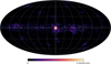 |
Fig. A.1 Map of the left term in Equation A.4. It shows the last iteration of the MAP RL solution in Figure 18. |
Here, we provide a more detailed discussion of the conditions under which the approximation introduced in Section 3.1 is valid. We focus on the TSV prior as an example. It is described as
 (A.1)
(A.1)
Its first and second derivatives can be calculated a
 (A.2)
(A.2)
 (A.3)
where N(σj) is the number of elements in σj. We note that for each pair (j, j′ ∈ σj), the term (λj − λj′)2 appears twice in the sum in Equation A.1, resulting in the coefficient 4 in the first derivative.
(A.3)
where N(σj) is the number of elements in σj. We note that for each pair (j, j′ ∈ σj), the term (λj − λj′)2 appears twice in the sum in Equation A.1, resulting in the coefficient 4 in the first derivative.
If we can assume that the first derivative and the sum of the response matrix change smoothly over the image  ), the condition that the updated image should satisfy (Equation 16) can be described as
 (A.4)
(A.4)
Figure A.1 shows the map of the left-hand term over the sky at the last iteration for the result with the 0.511 MeV thin disk model shown in Figure 18. The maximum value was ∼5 × 10⁻³, confirming that the condition for the approximation was satisfied in this case.
Appendix B Reconstructed 0.511 MeV images with different parameters
Figure B.1 shows the reconstructed 0.511 MeV images using various parameter values in the prior. The images surrounded by red boxes are candidates for the optimal solution derived from the L-curve method. The solid line surrounds the optimal solution, while the dashed line surrounds the second candidate.
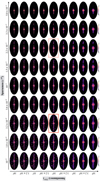 |
Fig. B.1 Reconstructed images of 0.511 MeV with different values for cTSV and cSP. |
Appendix C Comparison between the model and the data in the CDS
Here, we check how well the reconstructed image (shown in the top right panel of Figure 18) reproduces the observed data in the CDS for the 511 keV thin disk model. Since the CDS is multidimensional, we projected the expected counts onto two axes: the Compton scattering angle (ϕ) and the scattered gamma-ray direction (ψξ).
Figure C.1 and C.2 compare these projected histograms with the actual simulation data. In both figures, the top panels show the expected counts from the background and signal (purple) and those from the signal alone (green), overlaid with the observed counts (black). The middle panels show the residuals between the model prediction and the data. The bottom panels show the difference between expected counts and data divided by the square root of the expected counts, denoted as χ in the figures.
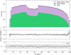 |
Fig. C.1 Comparison between model predictions and observed data for the 511 keV thin disk model, projected onto the ϕ axis. |
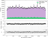 |
Fig. C.2 Same as Figure C.1, but projected onto the ψξ axis. For better visualization, the histograms are rebinned every 16 bins. |
The unbinned analysis, or the photon list approach, is also possible but will be subject of future publications.
The presented algorithm is implemented in the cosipy library, a highlevel analysis software for COSI. The codes are available at https://github.com/cositools/cosipy
These datasets are publicly available as a part of the second data challenge of the COSI project (Martinez 2023). The details are described at https://github.com/cositools/cosi-data-challenge-2
SAA particles could cause non-negligible background events, which will be addressed in future work. The simulation includes the veto shield by the BGO detectors. More details about the background simulations can be seen at https://github.com/cositools/cosi-data-challenge-2/tree/main/backgrounds
All Tables
Number of events filled in a histogram for the three-month simulation of each source distribution.
All Figures
|
Fig. 1 COSI payload design (top) and a schematic of the mass model used in our simulation (bottom). |
| In the text | |
|
Fig. 2 Schematic of Compton Data Space (Kierans 2018). The left panel shows a photon scattering in a detector with the scattering angle ϕ and the scattered gamma-ray direction (ψ, χ). The source position (ψ0, χ0) and photon interaction points are shown. Photons from this source make a cone with a 90° opening angle in the CDS, as shown on the right panel. The apex of the cone corresponds to the source location. |
| In the text | |
|
Fig. 3 Exposure maps for the three targets with three-month observations in Galactic coordinates. The exposures for 44Ti, 26Al, and 0.511 MeV are shown from top to bottom. The values represent the effective area integrated over both the observation time and the solid angle of each pixel. The solid angle per pixel is 4.1 × 10⁻³ sr, and the number of pixels is 3072. The range of the color bar is different in each case. It should be noted that the color bars of the images shown in this paper are in the log scale. |
| In the text | |
|
Fig. 4 Reconstructed images of 44Ti with different values for cSP. The left top panel shows the injected model for 44Ti. From the next to bottom right, cSP is set to 10−4, 10−2, 3 × 10⁻², 1 × 10⁻¹, and 2 × 10⁻¹. |
| In the text | |
|
Fig. 5 L-curve for the sparse prior. The x-axis shows the sparseness defined as ∑j log λj, while the y-axis shows the resulting log-likelihood. |
| In the text | |
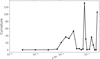 |
Fig. 6 Curvature of the L-curve shown in Figure 5 plotted against cSP. |
| In the text | |
|
Fig. 7 Log-posterior and log-likelihood for each iteration. Here, cSP is set to 10−2. |
| In the text | |
|
Fig. 8 Reconstructed flux compared with the simulated one. The solid line corresponds to using the flat prior distribution for the background normalization, while the dashed line is for the prior distribution with 0.1% accuracy. |
| In the text | |
|
Fig. 9 Flux outside the source. |
| In the text | |
|
Fig. 10 Optimization of the background normalization. |
| In the text | |
|
Fig. 11 Reconstructed images of 26Al with different values for cTSV. From top left to bottom right, cTSV is set to 104, 105, 3.16 × 10⁵, 106, 3.16 × 10⁶, and 107. The injected model is shown in Figure 14. |
| In the text | |
|
Fig. 12 L-curve for the smooth prior. The x-axis shows the total squared variation, while the y-axis shows the resulting log-likelihood. |
| In the text | |
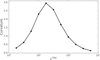 |
Fig. 13 Curvature of the L-curve shown in Figure 12 plotted against cTSV. |
| In the text | |
|
Fig. 14 Comparison between the reconstructed images obtained with different methods. The images are in the units of ph/cm2/s/sr. The top shows the injected model for the 26Al map, while the middle and bottom show the reconstructed image with the proposed algorithm and the conventional RL algorithm, respectively. |
| In the text | |
|
Fig. 15 Reconstructed 26Al fluxes along the Galactic longitude (top) and latitude (bottom). |
| In the text | |
|
Fig. 16 Two-dimensional L-curve for the sparse and smooth priors. The bottom plane corresponds to the smoothness and sparseness, while the z-axis shows the resulting log-likelihood. The black point corresponds to the optimal solution we presented in the main text. |
| In the text | |
|
Fig. 17 Curvature plots for the two-dimensional L-curve shown in Figure 16. Top: Curvature along cTSV with cSP fixed at its optimal value (3.2 × 10⁻²). Bottom: curvature along cSP with cTSV fixed at its optimal value (104). |
| In the text | |
|
Fig. 18 Comparison between the reconstructed 0.511 MeV images with different methods. The images are in the unit of ph/cm2/s/sr. The top left shows the injected thin model, while the reconstructed images with the proposed method, the conventional RL, and the RL using a Gaussian filter are shown on the top right, bottom left, and bottom right panels, respectively. Following the same discussion in Section 5.2.1, each pixel suffers from the Poisson fluctuation of ∼1000 background events (= 2.09 × 10⁶/3072) with a typical exposure of 3.5 × 105 cm2 s sr on a pixel, which corresponds to a noise level of ∼10−4 ph cm−2 s−1 sr−1 in the reconstructed image. |
| In the text | |
|
Fig. 19 Reconstructed 0.511 MeV fluxes along the Galactic longitude (left) and latitude (right). When plotting the model line, the flux from the point source in Table 1 is blurred with the pixel size of the image (∼3.7 degrees). |
| In the text | |
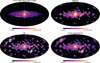 |
Fig. 20 Same as Figure 18 but for the thick disk model. |
| In the text | |
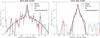 |
Fig. 21 Same as Figure 19 but for the thick disk model. |
| In the text | |
|
Fig. A.1 Map of the left term in Equation A.4. It shows the last iteration of the MAP RL solution in Figure 18. |
| In the text | |
|
Fig. B.1 Reconstructed images of 0.511 MeV with different values for cTSV and cSP. |
| In the text | |
|
Fig. C.1 Comparison between model predictions and observed data for the 511 keV thin disk model, projected onto the ϕ axis. |
| In the text | |
|
Fig. C.2 Same as Figure C.1, but projected onto the ψξ axis. For better visualization, the histograms are rebinned every 16 bins. |
| In the text | |
Current usage metrics show cumulative count of Article Views (full-text article views including HTML views, PDF and ePub downloads, according to the available data) and Abstracts Views on Vision4Press platform.
Data correspond to usage on the plateform after 2015. The current usage metrics is available 48-96 hours after online publication and is updated daily on week days.
Initial download of the metrics may take a while.