| Issue |
A&A
Volume 697, May 2025
|
|
|---|---|---|
| Article Number | A154 | |
| Number of page(s) | 13 | |
| Section | Stellar structure and evolution | |
| DOI | https://doi.org/10.1051/0004-6361/202452817 | |
| Published online | 14 May 2025 | |
Connections between the cycle-to-cycle light curve and O−C variations of non-Blazhko RR Lyrae stars
1
Konkoly Observatory, HUN-REN Research Centre for Astronomy and Earth Sciences, MTA Centre of Excellence, Konkoly Thege u. 15-17., 1121 Budapest, Hungary
2
Department of Astrophysical Sciences, Princeton University Peyton Hall, 4 Ivy Lane, Princeton, NJ 08544, USA
3
ELTE Eötvös Loránd University, Institute of Physics and Astronomy, 1117, Pázmány Péter sétány 1/A, Budapest, Hungary
⋆ Corresponding author: This email address is being protected from spambots. You need JavaScript enabled to view it.
Received:
30
October
2024
Accepted:
22
March
2025
Abstract
Context. It is widely known that if the durations of the consecutive cycles of a pulsating star vary in a random fashion, the O−C diagram could show quasi-periodic or irregular variations, even when the actual average period is constant. It has been hypothesised that the period variation observed in many RR Lyrae stars, which are much faster and stronger than would otherwise be explained by an evolutionary origin, could actually be caused by this cycle-to-cycle (C2C) variation effect. So far, quantitative studies have been scarce and space data have not been used to investigate this topic.
Aims. Our primary goal is to quantitatively analyse the O−C diagrams of RR Lyrae stars obtained from space photometry and explained by quasi-periodic or irregular periodic variations to see whether they can be explained by random fluctuations in pulsation cycle length, without assuming real period variations.
Methods. We fit statistical models to the O−C diagrams and tested their validity and fit. The necessary analysis of the light curves was performed using standard Fourier methods.
Results. We found that the vast majority of the O–C curves can be satisfactorily explained by assuming timing noise and the C2C variation without a real mean period variation. We have shown that the strength of the C2C variation is strongly dependent on the pulsation period and metallicity. These correlations suggest that turbulent convection may be behind the C2C variation. The additional frequencies of some RR Lyrae stars and their variation over time play only a marginal role in O−Cs. We have established new arguments to support the idea that the phase jump phenomenon in RRc stars is, in fact, a continuous change; moreover, we find it could also be caused by the C2C variation.
Key words: methods: data analysis / techniques: photometric / stars: oscillations / stars: variables: RR Lyrae
© The Authors 2025
 Open Access article, published by EDP Sciences, under the terms of the Creative Commons Attribution License (https://creativecommons.org/licenses/by/4.0), which permits unrestricted use, distribution, and reproduction in any medium, provided the original work is properly cited.
This article is published in open access under the Subscribe to Open model. This email address is being protected from spambots. You need JavaScript enabled to view it. to support open access publication.
1. Introduction
The period changes that characterise variable stars have been extensively studied and this is also the case for classical radially pulsating variable stars, such as Cepheids or RR Lyrae stars. These studies are typically aimed at finding period changes due to stellar evolution, detecting possible companions, and so on. These variations are long time-scales and/or are strictly periodic. However, pulsating variables are not precise clocks. Their consecutive pulsation cycles may slightly differ from each other. The fact that this might be the case has been suspected for a very long time, but for most variable types, it could only be proven by the latest, highly precise space photometric measurements.
The random period changes were investigated first by Eddington & Plakidis (1929). For long-period Mira variables, it was shown early on that successive pulsation cycle durations actually fluctuate randomly by 1–2% (Plakidis 1932, 1933). For shorter period variables, however, we had to wait for space photometry to find similar variations. Derekas et al. (2012) detected a period jitter on V1154 Cyg, which is the only classical Cepheid star investigated as part of the original Kepler mission (Borucki et al. 2010). Then, the cycle-to-cycle (C2C) variations were shown for further different sub-types of Cepheids in the data of the K2 (Howell et al. 2014), MOST (Evans et al. 2015), and TESS (Ricker et al. 2015) missions (Plachy et al. 2017, 2021). RR Lyrae stars have shorter periods than Cepheids, therefore, only high-cadence measurements are suitable for the direct detection of the C2C variation effect, even in space photometry, as this is the guarantee for a proper coverage of the light curve. Using 32-second (over-sampled) data of CoRoT (Baglin et al. 2006) and 1-minute short-cadence (SC) observations of Kepler space telescopes, C2C light curve variations were definitively found for non-Blazhko RRab stars by Benkő et al. (2016, 2019).
Traditionally, O−C diagrams have been used to detect period changes. The basic principle is simple: we let Ci be the time of the ith well-defined phase of a light curve (e.g. maximum, midpoint of the ascending branch, minimum), calculated by taking i cycles from a starting time, t0, with a constant period, P. The actual observed time of the same phase is denoted by Oi. Plotting the difference (O − C)i as a function of time gives us the O−C diagram. For a more detailed overview of the method, we refer to Sterken (2005). Using the O − C diagram, we are actually exploiting the fact that a period change always causes a change in the observed phase. If the period, P, varies over time, t, it is easy to see from the definition of O−C that
 (1)
(1)
where ⟨P⟩ indicates the average period. This formula illustrates the cumulative nature of O–C diagrams, which are helpful in detecting small changes by accumulating them over many pulsation cycles.
It is true that period changes cause changes in the observed phase (and, hence, changes in the O−C), but the O−C diagram could also show systematic changes when the average period is constant. This is an established phenomenon and Sterne (1934) was perhaps the first to point out that a random period fluctuation could cause O−Cs to change in a way that could be described by a random walk process. Balázs-Detre & Detre (1965) already used this phenomenon to explain the strong, irregular O−C variations observed in many RR Lyrae stars, which cannot be explained on the basis of an evolutionary origin. Subsequently, a series of papers have been published to discuss in detail the various mathematical and practical aspects of the problem (Lombard & Koen 1993; Koen & Lombard 1993; Koen 1996, 2006).
Recently, O−C diagrams of RR Lyrae stars from space photometric data series were published, showing quasi-periodic and irregular variations in addition to periodic ones (Benkő et al. 2019, 2023). In this paper, we address the extent to which these phenomena can be related to C2C variations of the light curves, with the aim of getting closer to determining the origin of these variations.
2. Method
Koen (2006) has shown that a quantitative analysis of the O−C diagrams can discriminate between the individual effects: the noise due to the phase determination error, the C2C variation of the light curve, and the actual period variation. The steps of the analysis are described in detail in Koen (2006) and only the necessary information is briefly summarised here. We begin with Koen’s statistical model for the instantaneous period Pi of the ith pulsation cycle, which is:
 (2)
(2)
where ⟨P⟩ is the constant average period. The sum represents a general model for the smooth period variation, where ξi are zero-mean uncorrelated random variables with a variance of σξ2; while the C2C variation is modelled by a zero-mean uncorrelated random variable, ηi, with a variance of ση2. Furthermore, we assume that the ei error in the timing of the phases is random, with a constant variance of σe2. Thus, we have:
 (3)
(3)
where Ti indicates the error-free timing value. The statistical model therefore depends on three random variables (ξ, η, and e) and three associated parameters (σξ, ση, and σe). In this framework, the O−C curves can be described in a fairly general way as
 (4)
(4)
where Ni and N indicate the ith and the total (N = Nk + 1) cumulative cycle numbers, respectively. Using the relation in Eq. (4) and applying different σ parameters, we find that curves that are very similar to the observed irregular O–C diagrams can be generated (see the figures in Koen 2005, 2006).
When modelling our observed O−C diagrams, we considered four scenarios for the possible phase changes. Since the determination of the data points is always subject to error the phase (or timing), noise is unavoidable: σe > 0. For the first model (M1), we assumed that only this timing noise is present, nothing else (ση = σξ = 0). In the second case (M2), we suppose that although the mean period does not change (σξ = 0), there is a random C2C variation in the light curve causing variation of the pulsation cycle duration (ση > 0). In the next model (M3), the average period varies (σξ > 0), but there is no C2C variation (ση = 0). Finally (M4), a period variation and C2C fluctuation are permitted simultaneously (ση > 0 and σξ > 0).
For each model, we needed to maximise the Gaussian log-likelihood function, as per
 (5)
(5)
where Σ = covZ,Z) is the covariance matrix of Z and its elements are defined as Zi = (O − C)i. Then we had to to calculate the Akaike (AIC) or Bayesian information criteria (BIC):
 (6)
(6)
 (7)
(7)
where p denotes the number of the free parameters of a certain model (p = 1, 2, or 3). The probability of the model is then:
 (8)
(8)
This procedure leads to the best-fitting (most likely) model. When fitting models, Koen (2006) defines the pseudo-residual as
 (9)
(9)
which plays a role similar to that of, for example, residuals in Fourier fits of light curves; for an optimal fitting, the pseudo-residual is a zero-mean, uncorrelated, random variable.
We developed a PYTHON code that implements the method described above. We have intensively relied on the NUMPY and SCIPY extensions of PYTHON (Harris et al. 2020; Virtanen et al. 2020). The input of the program is the O−C diagram, which is formed by a linear transformation if necessary to satisfy (O − C)0 = (O − C)k + 1 = 0. The programme tests the four statistical models maximising the log-likelihood functions with the unknown σ parameters. We tried several bound-constrained maximization algorithms and the Nelder-Mead method of SCIPY (Gao & Han 2012) was found to be suitable to address our problem. We calculated the statistical probability (Eq. (8)) of each model using both the AIC and BIC. The program also examines the fit of each model and provides an estimate of the normality of the pseudo-residuals using the SCIPY.STATS.SHAPIRO routine (Shapiro & Wilk 1965; Royston 1995).
3. Statistical models for RRab stars
A significant fraction of RR Lyrae stars show a characteristic simultaneous amplitude and frequency variation with a period (or periods) that is much longer than the pulsation period. For a detailed discussion of this so-called Blazhko effect, we refer to Smolec et al. (2016) or Kovács (2016). The effect usually dominates the O−C diagram of these stars, showing (multi)periodic signal shapes (Benkő et al. 2014). Throughout this paper, we focus on non-Blazhko stars, as we are now mainly interested in non-periodic phenomena.
3.1. O–C curves of RRab stars
When Benkő et al. (2019) detected the C2C light curve variation of non-Blazhko Kepler RRab stars directly, the amplitude and light curve shape variation were found to sufficient for detecting such C2C variation. It is important to point out that variation in the shape of the light curve does not necessarily imply an O−C variation. To verify that this type of variation is indeed at work, the light curve must change to the extent that the length of the pulsation cycle changes, which can then be detected on the O−C diagram. However, experience has shown that the C2C light curve changes of pulsating variables always occur in this way. The O−C diagrams calculated from the Kepler long-cadence (LC, ∼29.5 min) data and their slightly transformed forms have also been published (see Figs. 13 and 14 in Benkő et al. 2019) and their Fourier analyses have been performed. Since most of the found frequencies appeared in more than one star, it was thought that they might be instrumental frequencies. However, Li et al. (2023a) presented several valuable arguments against these identifications: (i) from a statistical analysis of these frequencies (see their Fig. 7), it has been concluded that the identification of all such frequencies with instrumental frequencies is unlikely; and (ii) the slopes of O−C curves containing similar (considered identical within error) frequencies are also very different, which would not be the case with respect to an instrumental effect.
We excluded V346 Lyr from the sample after it turned out to be a Blazhko star and we tested the remaining 18 stars with the statistical model described above. We used the original O−C curves; that is, in contrast to the diagrams presented in Benkő et al. (2019), we did not transform out any longer term changes. On the contrary, the four significant high-frequency (f > 0.01 d−1) signals published for NR Lyr, FN Lyr, and V1510 Cyg were pre-whitened from the data, since these signals are definitely related to some periodic phenomenon and as such are not the subject of the present study.
The results of the analysis are summarised in Table 1 and Fig. A.1. The name and main pulsation period of the star are given in the first two columns of Table 1. The next two columns contain the σe and ση parameters of the optimal model. The optimal model is M2 in 16 out of 18 cases (89%), that is, the O−C curve can be described by C2C variation and phase noise. In two cases (V175 Cyg and KIC 9717032), the combined M4 model proved to be the best. In both cases, there is a strong linear trend in the O−C curves. However, a very similar change can be seen in the O−C curves of V368 Lyr, V1510 Cyg and AW Dra; however, for these stars, the M2 model is the most likely. This underlines the need for quantitative analysis of O−C curves beyond simple visual inspection.
Kepler non-Blazhko RRab stars.
We note that the probabilities, pjC, obtained for the M2 model are between 0.63 and 0.85, while for the same stars the probability of the M4 model is between 0.15 and 0.37. When calculating the pjC probabilities, the use of AIC and BIC suggests a different model in only one case: for KIC 9717032, AIC suggests the model M4 (p4AIC = 0.85), while BIC suggests the model M2 (p2BIC = 0.66). In this case, following Koen (1996), we accepted the model obtained from the AIC formula. The last column shows the additional frequencies that appear permanently for these stars, with the temporary ones given in parentheses.
In addition to Table 1, Fig. A.1 illustrates the analysis performed in this work. The first columns of the figures show the input data for the untransformed O−C curves. The panels in the second column show the values of ui, the pseudo-residuals defined by the formula in Eq. (9) for the best model. If a model is optimal, the pseudo-residuals are zero-mean uncorrelated random variables. A possible verification of this is shown in the panels of the third column: here, we give the normalised distribution of the pseudo-residuals compared to the probability density function of the standard normal distribution with σ = 1 variance. The p-value of the Shapiro-Wilk test is also indicated in each panel. The test is usually used so that if the p-value is greater than 0.05, it suggests that the data does not significantly deviate from normality. In our case 0.09 < p < 0.96, which means that all the pseudo-residuals are a good approximation of a random variable with normal distribution. In principle, it is possible that the pseudo-residual associated with the optimal model is not white noise. In this case, further tests would be needed to accept or reject the model; fortunately, this was not the case for our samples.
3.2. C2C variation and the physical parameters of RRab stars
On the one hand, our statistical model gives the value of the phase noise σe for each O−C diagram. On the other hand, when the O−C values were calculated from the light curves, the error of the individual O−C points was also estimated. It may be worth comparing these two error estimates. We calculated the average and the standard deviation of the individual O−C point errors for each star and denoted this by ⟨σ(O − C)⟩ and μO − C, respectively. In the horizontal axis of Fig. 1, we show the σe values for each RRab star; whereas on the vertical axis we show the values of ⟨σ(O − C)⟩ and their standard deviation, μO − C, with the error bars, as defined above. We see that the two error estimates give similar values; namely, within 3μO − C they are identical and for the majority, the difference is within 1μO − c.
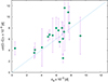 |
Fig. 1. Estimations of the phase noise σe from the statistical fit (horizontal scale) with respect to the averaged O−C determination error (vertical scale) for each RRab star in the sample (dots). The solid blue line shows a linear with slope one for comparison. |
To unravel the origin of the C2C variation, we plotted the dependence of the ση parameter characterising the strength of the effect on some important physical parameters in Fig 2. In Fig. 2, we show the dependences on the main period, P0, metallicity, [M/H], effective temperature, Teff, surface gravitational acceleration, log g, micro-turbulence, ξt and macro-turbulence, νmac. Except for the period, the other parameter values were taken from Table 9 of Nemec et al. (2013), determined from high-resolution spectra obtained with CFHT and Keck telescopes. The stars are marked with different symbols according to their additional frequency contents. The presence of low-amplitude additional frequencies does not exclude stars from the analysis because, as shown by Benkő et al. 2019, they do not significantly affect C2C detections. Filled circles indicate stars that do not show additional frequencies, while stars containing the f1 and f2 radial first and second overtone frequencies are represented by rectangles and triangles, respectively. The sizes of the symbols indicate the approximate errors.
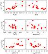 |
Fig. 2. Strength of C2C variation as a function of the main period and some physical parameters for Kepler RRab stars. The stars with no additional frequencies, f1 and f2 frequencies are plotted as filled circles, rectangles and triangles, respectively. The green line shows the significant correlation between period and ση. |
Some of the panels in Fig. 2 suggest relations. Since the parameters given here are not independent, a standard multiple linear regression was used to find true significant relationships. In practice, we used the statsmodels PYTHON package (Seabold & Perktold 2010). First, all six parameters (P0, [M/H], Teff, log g, ξt, νmac) were fitted simultaneously. The obtained p-value of the F-statistic (pF = 0.012) indicates that at least one of the fitted parameters has a significant effect on the dependent variable, ση. Looking at the results for each parameter, we see that there is indeed a positive correlation with the period. The probability of the t-statistic is pt = 0.021. For other variables we do not see a significant correlation (all other pt > 0.05). The obtained linear relationship for the period is
 (10)
(10)
shown by the green line in the top left panel of Fig. 2. Here, the amplitude of the C2C variation is higher for stars with longer periods. Both ση and the period, P0, are given in units of days.
As mentioned in the introduction, it has long been known that the C2C variation of the longest period pulsating variables (e.g. Miras) is the strongest relative to the pulsation cycle, compared to other pulsators (e.g. Cepheids). A linear period dependence within a variable type was published also for the case of Mira stars (Koen & Lombard 2004). Balázs-Detre & Detre (1965) suggested that for RRab stars, the effect is strongest at intermediate periods (0.11% between 0.52 and 0.58 d) and smaller (0.09 and 0.05%) at shorter and longer periods. These percentages represent ∼3.3 – 6 × 10⁻⁴ d, which is about an order of magnitude larger than the ones we obtained, but their statistical model was simpler than the one used here; they did not account for phase noise, but attributed the entire random variation to the C2C effect.
Unfortunately, no significant correlations with the real physical parameters were obtained. One reason for this is likely the small number of elements in our sample. This is supported by the fact that if we omit AW Dra data from the fit (that appear to be outliers), we do not get significant correlations with any of the variables; however, P0, Teff and [M/H] give similar probabilities (pt ∼ 0.16 − 0.19).
4. RRc stars
4.1. Possible C2C variation in RRc stars
Direct photometric detections of the C2C variations have not been reported for any RR Lyrae stars that pulsate in the first radial overtone mode (RRc stars). After reviewing the available data series, we focussed on the well-sampled ones where there is no other variation (caused by additional modes or the Blazhko effect) than the main pulsation, which could interfere with our analysis. Despite the fact that Benkő et al. (2019) found that the additional frequencies and C2C variations interact only marginally in RRab stars, this is not known for RRc stars, as the additional frequencies in these stars are of different types and have larger relative amplitudes compared to the main frequency. Therefore, to detect C2C directly, it is necessary to first look for ‘clean’ cases, namely, those that are free of additional frequencies. On the additional frequency content of RR Lyrae stars and their differences by subtypes, we refer, for instance, to the reviews by Molnár et al. (2017) or Plachy et al. (2021).
Checking the available high cadence data from CoRoT (Baglin et al. 2006) and the original Kepler mission (Borucki et al. 2010), we found no RRc star that did not show an additional frequency and/or the Blazhko effect. The Kepler extended mission, K2 (Howell et al. 2014), however, observed several such RRc stars in 1-minute short-cadence (SC) mode. A review of guest observer (GO) data targeting RR Lyrae SC observations found 34 candidates. The candidates were compared with the results of Netzel et al. (2023) and two stars were identified, showing neither the Blazhko effect nor any additional frequencies: EPIC 212640806 (Kp = 15.889 mag) and EPIC 249685909 (Kp = 12.724 mag). To produce the best possible light curves, the automated extended aperture photometry method (Bódi et al. 2022) was applied to the original CCD frame parts (i.e. ‘pixel data’) of both stars.
The light curves for the fluxes were analysed with the Period04 software package (Lenz & Breger 2005). After pre-whitening the data of EPIC 212640806 with the main frequency and its significant harmonics, side peaks appear around the harmonics in the Fourier spectrum. From the residual light curve, it is clear that these side peaks are not caused by the Blazhko effect, but by some other effect, such as an instrumental problem. Otherwise, there is no structure in the residual light curve, only noise. This is consistent with the fact that C2C variations can only be detected up to a certain brightness limit (Benkő et al. 2019). The brighter candidate, EPIC 249685909, was found to have low amplitude but significant frequencies in its residual spectrum after a more detailed analysis. In other words, we have not found any RRc stars in K2 that are suitable for direct detection of C2C variation.
The initial half-hour exposure time of the full-frame images of the TESS space telescope (Ricker et al. 2015) gave inadequate phase coverage for our purposes. Although five non-Blazhko RRc stars were measured by TESS at the request of the RR Lyrae working group GO proposal with a sample of 120 seconds, unfortunately, they all contain additional frequencies. However, after the second extension of the mission (from 1 September 2022), the default exposure time was reduced to 200 s. This sampling density may be sufficient. From the TESS RRc sample of Benkő et al. (2023), we selected stars that did not show any extra signals beyond the main frequency and their harmonics. We found 27 such stars brighter than 13.5 mag, for which the quick look pipeline photometry is available (Huang et al. 2020a,b; Kunimoto et al. 2021, 2022). These photometric data series were examined to look for signs of C2C variation.
Taking into account the difference in apertures (10.5 cm for TESS, 95 cm for Kepler) and exposure times (58.9 s for Kepler SC and 200 s for TESS), we estimated the detection limit of TESS to be about 3.5 mag brighter than Kepler. For the Kepler RRab stars, the detection limit of the effect was found to be Kp ∼ 15 mag (Benkő et al. 2019) which means that only the brightest TESS RRc stars are candidates for the detection of the C2C effect. The C2C variations are well traced on the residual light curves, from which the main frequency and its significant (10–15) harmonics have been pre-whitened; this is illustrated in Figs. 1 and 2 in the paper by Benkő et al. (2019). Figure 3 shows the 5-day chunks of the residual light curves of the three brightest stars in our sample. Unfortunately, none of them show any definite structure. In the case of RRab stars, because of the different strengths of the C2C variation in different phases of the light curve, we can see a defined structure in the residuals (see Figs. 1 and 2 in Benkő et al. 2019).
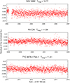 |
Fig. 3. Segments (of five days) of the residual flux curves of the three brightest TESS RRc stars after the main frequency and its significant harmonics that have been pre-whitened from the data. The relative flux scale is the same for all three stars. There is no detectable structure indicating a C2C variation. |
Thus, it appears that there is currently no photometric data set from which the C2C variation of RRc stars can be directly detected. However, indirect analysis of C2C variations using O−C diagrams can be done in a similar way to the approach for RRab stars.
4.2. O−C diagrams of RRc stars
Benkő et al. (2023) published phase variations on a one-year timescale for 32 RRc stars (see their Fig. 14) in the TESS Continuous Viewing Zone (CVZ). From these phase variations, we constructed the O−C diagrams for the 26 non-Blazhko stars. Similarly to the RRab stars, the evident short-period signals (with a frequency of f > 0.03 d−1) were also removed. From the O−C curves of each star, 1–5 (on average 2) such frequencies were pre-whitened (for the frequency values see Table 6. in Benkő et al. 2023). The resulting curves were used to fit the statistical models described above for RRab stars. The O−C diagrams, the pseudo-residuals corresponding to the best-fitting models, and their distributions are shown in Fig. B.1. The numerical results are summarised in Table 2.
TESS RRc stars.
Remarkably, the value of ση is (on average) an order of magnitude larger than for RRab stars, namely: ⟨σ(RRc)η⟩ = 1.20 × 10⁻⁴ versus ⟨σ(RRab)η⟩ = 1.76 × 10⁻⁵. The study of Balázs-Detre & Detre (1965) gave 0.04% for the estimated C2C period variation of RRc stars, which means ση ≈ 1.0 − 1.6 × 10⁻⁴, which is thus in agreement with the result obtained here.
For 21 of the 26 RRc stars, the optimal model, M2 (81%), that is the O−C curve, can be described by the C2C variation and the phase noise. For three cases (Gaia DR2 1650042086261498880, Gaia DR2 5285510178935677312, and [SHM2017] J285.32992+67.89109) the combined (M4) model proved to be the best; whereas for two stars (Gaia DR2 5476969341269561344 and Gaia DR2 5486632674089049472), the combination of phase noise and a real period variation was found to be the most probable.
4.3. C2C variation and the physical parameters for RRc stars
For RRab stars, we found a correlation between the strength of the C2C variations and the main pulsation period. We also attempted to find correlations for the RRc sample.
Unfortunately, high-resolution spectroscopy is not available for our RRc stars. Therefore, we used the calibration of Li et al. (2023b), who determined [Fe/H] values from Gaia DR3 G-band photometry. Since not all of our stars were included in their table, we used the Li et al. formula:
![Mathematical equation: $$ \begin{aligned} \mathrm{[Fe/H]} =-1.737 - 9.968(P_1-0.3) - 5.041(R_{21}-0.2) .\end{aligned} $$](/articles/aa/full_html/2025/05/aa52817-24/aa52817-24-eq11.gif) (11)
(11)
Here, the P1 is the mean period calculated from the TESS light curves and R21 = A(2f1)/A(f1) is the amplitude ratio of the G-band light curves. For the stars in the Li et al. (2023b) table, our calculated and published [Fe/H] values agree within a few hundredths of a percent, well below the 1σ error limit (∼0.2–0.3 dex). The applied [Fe/H] values are listed in column 9 in Table 2.
The effective temperatures were determined by the algorithm of Casagrande et al. (2021) using Gaia DR3 and 2MASS colours and shown in column 7 of Table 2. The values are rounded to ten, the average error is ∼150 K. In the most recent publication of the LAMOST Survey of RR Lyrae (Wang et al. 2024), only two stars from our sample are included, so the log g values are taken from Gaia DR3 (Gaia Collaboration 2023) as the most extensive homogeneous source; even so, we do not have data on six of our stars (column 8 in Table 2). We used the ‘GSP-Phot’ values estimated from the BP − RP colour indices.
In the panels of Fig. 4, we plotted the C2C variation strength parameter, ση, as a function of the main period, P1, the metallicity, [Fe/H], the effective temperature, Teff, and the surface gravitational acceleration, log g. The physical parameters used are listed in Table 2. The stars are marked with different symbols according to their additional frequency content. Filled circles, squares, triangles, or diamonds represent stars with no additional frequency, one additional frequency (f60 or f61), a f68 frequency, and two frequencies (both f61 and f63), respectively.
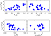 |
Fig. 4. Parameter ση characterising the C2C variation for the stars of the RRc sample as a function of the main pulsation period, P1, metallicity, [Fe/H], effective temperature, Teff, and log g. The different symbols show the additional frequency content of the stars (see text for the details). |
To search for relations, as for the RRab stars, we first performed simultaneous multiple linear regressions with all four parameters: P1, [Fe/H], Teff, and log g. Strong (pt < 0.001) significant linear dependence results with period and metallicity were obtained according to the following formula:
![Mathematical equation: $$ \begin{aligned} \sigma _\eta =-5.67(\pm 0.86)+27.87(\pm 3.04)P_1+1.42(\pm 0.21)\mathrm{[Fe/H]} . \end{aligned} $$](/articles/aa/full_html/2025/05/aa52817-24/aa52817-24-eq12.gif) (12)
(12)
ση and P1 are measured in days and [Fe/H] in the usual dimensionless quantity (dex). No correlation was found for effective temperature or log g. However, we note that stars with two additional frequencies (diamonds in Fig. 4) are grouped at lower temperatures (bottom left panel). This was previously mentioned by Benkő et al. (2023), based on the period distribution of these stars, but has yet not been investigated in detail. The lack of correlation with log g may also be due to the known fact that the Gaia physical data for horizontal branch stars such as RR Lyrae (cf. Table 2 data and Fig. 14 in Molnár et al. 2023) are not entirely accurate.
4.4. The ‘phase jump’ phenomenon
Longer-term ground-based observations of some RRc stars, observing the stars over several seasons, have found that while the shape of the light curve appears to be constant, no single period can describe the light curves. However, assuming that a phase jump occurred in the unobserved time interval, the light curves can be folded perfectly (e.g. Wils et al. 2007; Wils 2008; Odell & Sreedhar 2016; Berdnikov et al. 2017). This behaviour is known as phase jump phenomenon. The long continuous data series of the Kepler space telescope suggested that the phenomenon is most likely not the consequence of a sudden jump, but rather the result of a continuous phase change (Moskalik et al. 2015; Sódor et al. 2017). For example, in the case of KIC 4064484, the phase is almost constant for ∼100 d and then it changes by 0.3 rad on a similar time scale of 100 days. After that, it stays at this level for about ∼200 d and then returns to almost the initial value again in 150–200 days (see Fig. 9 in Moskalik et al. 2015). Such a phase change from the Earth’s surface, observed seasonally, could be modelled by at least two abrupt phase jumps. Continuous phase changes similar to KIC 4064484 can be seen on our several TESS O−C curves (e.g. CRTS J165523.7+573029, NSVS 3117163, or CRTS J165930.9+650919 in Fig. B.1).
The above explanation of the phase jump phenomenon was first proposed by Benkő et al. (2023). Here we decided to take two further steps to understand what causes the observed phenomenon. We find that (i) the times corresponding to the phase jumps range from a few seconds to tens of minutes, that is: between ∼10−4 and ∼10−2 d. The vertical scales of the O−C diagrams in Fig. B.1 are located exactly in this interval. In other words, the phenomenon is not only qualitatively possible, but the observed O−C values are also quantitatively appropriate; (ii) since we found that the majority of the O−Cs can be explained by the C2C variations of the light curve, we can conclude that the jumps observed in the ground-based data are nothing more than the result of incomplete observations of (continuous) phase changes due to C2C variations. This hypothesis is supported by the fact that the shape of the light curve of phase jump stars (by definition) does not change, at least within the accuracy of ground-based measurements.
5. Discussion
As we seen in this paper, 81–89% of the O−C variations in our RR Lyrae sample (16 stars out of 18 RRab and 21 stars out of 26 RRc) can be explained purely on the basis of timing noise and C2C variations of the light curves without assuming a real period change. Thus, we consider a plausible explanation for the physical origin of the C2C variation phenomenon. The one-dimensional theoretical pulsation models (Buchler et al. 1997; Feuchtinger 1999; Smolec & Moskalik 2008) is not able to reproduce the C2C variations: after reaching the limit cycle, these models are strictly repetitive. Sweigart & Renzini (1979) explained the effect by random mixing events in the semi-convective layer around the convective core. The hypothetical mechanism is as follows: mixing causes a change in the layering of the chemical composition. As a result, the hydrostatic equilibrium of the star changes: the radius of the star (and, hence, the pulsation period) changes. Deasy & Wayman (1985) mentioned several explanations for the random periodic variations in Cepheids: one is the interaction of turbulent convection and pulsation, while the other is the mass loss. They have not carried out quantitative studies of either, but Cox (1998) has shown via theoretical calculations that small changes in the He gradient at the bottom of the H and He convection zones can indeed cause sufficient period changes.
The correlations between the parameter ση, indicating the strength of C2C variation, and the period calculated via Eqs. (10) and (12) might be explained qualitatively on the basis of convection. As shown by Bellinger et al. (2020), the period (and amplitude) of an RR Lyrae star is mostly determined by the effective temperature. Our own analysis showed well that there was a strong multi-colinearity in the simultaneous regression of period and effective temperature, demonstrating that these are highly correlated parameters. This is illustrated in Fig. 5, where we plot the fundamentalised period (Pfund = P0, or P1/0.745) of the stars in our sample as a function of log Teff. It can be seen that both the RRab and RRc samples are relatively small individually, but taken altogether, a strong non-linear relationship is evident: longer periods are typically associated with lower temperatures and vice versa. Then, by relating ση(P) functions to temperature, we find that the strength of the C2C variation increases towards lower temperatures. However, we know that the strength of convection also increases with decreasing temperature. Furthermore, there is no such obvious explanation for the correlation with metallicity. Metallicity affects the internal structure of the star and the correlation reported here might be a consequence of that.
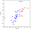 |
Fig. 5. Relation between the fundamentalised period, Pfund, and the effective temperature for the stars in our sample. Red rectangles: RRab stars, blue circles: RRc stars. |
Thus, indications suggest that convection may be behind the C2C variation phenomenon. This is supported by the fact that despite their shorter pulsation periods and higher effective temperatures, RRc stars show (on average) stronger C2C variations by an order of magnitude. Indeed, it is known that while convection interacting with pulsation is significant only in certain pulsation phases in RRab stars, convection is continuously present in RRc stars (Gautschy 2019). The theoretical description of the interaction between pulsation and convection is still a topic of ongoing research (Kovács et al. 2023, 2024). This question can only be satisfactorily resolved in the future using multidimensional pulsation codes. Significant initial steps have been made with such codes (Geroux & Deupree 2015; Mundprecht et al. 2015; Kupka & Muthsam 2017), but the descriptions are far from complete. Hopefully, these studies will be able to reproduce C2C variations in a natural way.
To describe the O−C curves, we had to assume actual period variation (models M3 or M4) for two RRab stars (11%) and five RRc stars (19%) among our studied stars. These period changes are rather slow, with a minimum timescale of half-a-year. If these are periodic variations, their period can vary from about a half a year to several years. The measured period variation is between 7.3 × 10⁻³ and 3.3 × 10⁻² d. Assuming periodic variation, these values are lower limits. Several explanations have been proposed for such long-period phase variations. Li & Qian (2014), Li et al. (2023a) explained the variation of FN Lyr, V894 Cyg, and V838 Cyg by low-mass companions around the stars; whereas Benkő et al. (2019) hypothesised that it could be an instrumental effect. FN Lyr and V894 Cyg are included in our sample and C2C variations seem to be a satisfactory explanation in both cases (noting that V838 Cyg shows a Blazhko effect and was therefore omitted by this work.) However, the assumption of binarity or a companion should always be considered for these types of changes. Since we are dealing with a strictly periodic signal in this case, with a time series of sufficient length (covering several complete cycles), such an assumption can be confirmed. If TESS does indeed continue its observations for 10-15 years, this could allow for the hypothesis to be tested for some stars.
6. Conclusions
Firstly, we start with the work of Benkő et al. (2019), who used the SC data of Kepler non-Blazhko RRab stars to show that the light curves of these stars vary slightly from cycle to cycle. In the current work described in this paper, we performed a statistical modelling of the O−C curves calculated from the LC data of the same stars. On this basis, we show that the vast majority of the O−C curves (16 out of 18 stars) can be satisfactorily explained by assuming timing noise and the C2C variation phenomenon without having to include a true mean period change.
Secondly, the statistical fits were not sensitive to the additional frequencies that appear in certain stars. This is consistent with the finding of Benkő et al. (2019) that the C2C variation effect dominates over the influence of the additional frequencies.
Thirdly, we have shown that the strength of the C2C variation is strongly dependent on the pulsation period: the effect is stronger for longer periods. The strength of the C2C variation in RRc stars depends also on metallicity. From the nature of the connections, we can suspect that turbulent convection may be behind the C2C variation.
Furthermore, the C2C variation of RRc stars could not be detected directly by comparing the successive pulsation cycles of the light curves (as was done for RRab stars) because no data series was found to meet all the necessary criteria. However, the long-term effects of the C2C variation on the O−C diagrams could be used to estimate the strength of the C2C variation, as for RRab stars. This was found to be on average an order of magnitude larger than for RRab stars, but the dependence on pulsation period is similar to the correlations found for RRab stars. Again, for 81% of the stars, the timing noise and the C2C variation were sufficient to explain the observed O−Cs.
Finally, considering the timescale and shape of the O−C variation in RRc stars, we suspect that the phase jumps found in ground-based observations are likely due to non-continuous observations of continuous phase variations caused by C2C variations.
Acknowledgments
This paper includes data collected by the Kepler and TESS missions. Funding for the missions are provided by the NASA Science Mission Directorate. The research was partially supported by the ‘SeismoLab’ KKP-137523 Élvonal grant of the Hungarian Research, Development and Innovation Office (NKFIH) and by the NKFIH excellence grant TKP2021-NKTA-64. Some PYTHON codes were developed with the help of ChatGPT 3.5. The authors thank the reviewer for her/his helpful suggestions and J. Bienias for his correction to the language.
References
- Baglin, A., Auvergne, M., Barge, P., et al. 2006, in The CoRoT Mission Pre-Launch Status - Stellar Seismology and Planet Finding, eds. M. Fridlund, A. Baglin, J. Lochard, & L. Conroy, ESA Spec. Publ., 1306, 33 [NASA ADS] [Google Scholar]
- Balázs-Detre, J., & Detre, L. 1965, Veroeffentlichungen der Remeis-Sternwarte zu Bamberg, 27, 184 [Google Scholar]
- Bellinger, E. P., Kanbur, S. M., Bhardwaj, A., & Marconi, M. 2020, MNRAS, 491, 4752 [NASA ADS] [CrossRef] [Google Scholar]
- Benkő, J. M., Plachy, E., Szabó, R., Molnár, L., & Kolláth, Z. 2014, ApJS, 213, 31 [CrossRef] [Google Scholar]
- Benkő, J. M., Szabó, R., Derekas, A., & Sódor, Á. 2016, MNRAS, 463, 1769 [CrossRef] [Google Scholar]
- Benkő, J. M., Jurcsik, J., & Derekas, A. 2019, MNRAS, 485, 5897 [CrossRef] [Google Scholar]
- Benkő, J. M., Plachy, E., Netzel, H., et al. 2023, MNRAS, 521, 443 [Google Scholar]
- Berdnikov, L. N., Dagne, T., Kniazev, A. Y., & Dambis, A. K. 2017, Inf. Bull. Variable Stars, 6212, 1 [Google Scholar]
- Bódi, A., Szabó, P., Plachy, E., Molnár, L., & Szabó, R. 2022, PASP, 134, 014503 [CrossRef] [Google Scholar]
- Borucki, W. J., Koch, D., Basri, G., et al. 2010, Science, 327, 977 [Google Scholar]
- Buchler, J. R., Kolláth, Z., & Marom, A. 1997, Ap&SS, 253, 139 [Google Scholar]
- Casagrande, L., Lin, J., Rains, A. D., et al. 2021, MNRAS, 507, 2684 [NASA ADS] [CrossRef] [Google Scholar]
- Cox, A. N. 1998, ApJ, 496, 246 [NASA ADS] [CrossRef] [Google Scholar]
- Deasy, H. P., & Wayman, P. A. 1985, MNRAS, 212, 395 [NASA ADS] [CrossRef] [Google Scholar]
- Derekas, A., Szabó, G. M., Berdnikov, L., et al. 2012, MNRAS, 425, 1312 [NASA ADS] [CrossRef] [Google Scholar]
- Eddington, A. S., & Plakidis, S. 1929, MNRAS, 90, 65 [NASA ADS] [CrossRef] [Google Scholar]
- Evans, N. R., Szabó, R., Derekas, A., et al. 2015, MNRAS, 446, 4008 [CrossRef] [Google Scholar]
- Feuchtinger, M. U. 1999, A&AS, 136, 217 [NASA ADS] [CrossRef] [EDP Sciences] [Google Scholar]
- Gaia Collaboration (Vallenari, A., et al.) 2023, A&A, 674, A1 [NASA ADS] [CrossRef] [EDP Sciences] [Google Scholar]
- Gao, F., & Han, L. 2012, Computat. Optim. Appl., 51, 259 [Google Scholar]
- Gautschy, A. 2019, ArXiv e-prints [arXiv:1909.10444] [Google Scholar]
- Geroux, C. M., & Deupree, R. G. 2015, ApJ, 800, 35 [NASA ADS] [CrossRef] [Google Scholar]
- Harris, C. R., Millman, K. J., van der Walt, S. J., et al. 2020, Nature, 585, 357 [NASA ADS] [CrossRef] [Google Scholar]
- Howell, S. B., Sobeck, C., Haas, M., et al. 2014, PASP, 126, 398 [Google Scholar]
- Huang, C. X., Vanderburg, A., Pál, A., et al. 2020a, Res. Notes Am. Astron. Soc., 4, 204 [Google Scholar]
- Huang, C. X., Vanderburg, A., Pál, A., et al. 2020b, Res. Notes Am. Astron. Soc., 4, 206 [Google Scholar]
- Koen, C. 1996, MNRAS, 283, 471 [Google Scholar]
- Koen, C. 2005, in The Light-Time Effect in Astrophysics: Causes and cures of the O-C diagram, ed. C. Sterken, ASP Conf. Ser., 335, 25 [Google Scholar]
- Koen, C. 2006, MNRAS, 365, 489 [Google Scholar]
- Koen, C., & Lombard, F. 1993, MNRAS, 263, 287 [Google Scholar]
- Koen, C., & Lombard, F. 2004, MNRAS, 353, 98 [Google Scholar]
- Kovács, G. 2016, Commmun. Konkoly Obs. Hungary, 105, 61 [NASA ADS] [Google Scholar]
- Kovács, G. B., Nuspl, J., & Szabó, R. 2023, MNRAS, 521, 4878 [CrossRef] [Google Scholar]
- Kovács, G. B., Nuspl, J., & Szabó, R. 2024, MNRAS, 527, L1 [Google Scholar]
- Kunimoto, M., Huang, C., Tey, E., et al. 2021, Res. Notes Am. Astron. Soc., 5, 234 [Google Scholar]
- Kunimoto, M., Tey, E., Fong, W., et al. 2022, Res. Notes Am. Astron. Soc., 6, 236 [Google Scholar]
- Kupka, F., & Muthsam, H. J. 2017, Liv. Rev. Comput. Astrophys., 3, 1 [Google Scholar]
- Lenz, P., & Breger, M. 2005, Commun. Asteroseismol., 146, 53 [Google Scholar]
- Li, L. J., & Qian, S. B. 2014, MNRAS, 444, 600 [CrossRef] [Google Scholar]
- Li, L. J., Qian, S. B., Shi, X. D., & Zhu, L. Y. 2023a, AJ, 166, 83 [Google Scholar]
- Li, X.-Y., Huang, Y., Liu, G.-C., Beers, T. C., & Zhang, H.-W. 2023b, ApJ, 944, 88 [NASA ADS] [CrossRef] [Google Scholar]
- Lombard, F., & Koen, C. 1993, MNRAS, 263, 309 [Google Scholar]
- Molnár, L., Plachy, E., Bódi, A., et al. 2023, A&A, 678, A104 [NASA ADS] [CrossRef] [EDP Sciences] [Google Scholar]
- Molnár, L., Plachy, E., Klagyivik, P., et al. 2017, Eur. Phys. J. Web Conf., 160, 04008 [CrossRef] [EDP Sciences] [Google Scholar]
- Moskalik, P., Smolec, R., Kolenberg, K., et al. 2015, MNRAS, 447, 2348 [NASA ADS] [CrossRef] [Google Scholar]
- Mundprecht, E., Muthsam, H. J., & Kupka, F. 2015, MNRAS, 449, 2539 [NASA ADS] [CrossRef] [Google Scholar]
- Nemec, J. M., Cohen, J. G., Ripepi, V., et al. 2013, ApJ, 773, 181 [CrossRef] [Google Scholar]
- Netzel, H., Molnár, L., Plachy, E., & Benkő, J. M. 2023, A&A, 677, A177 [NASA ADS] [CrossRef] [EDP Sciences] [Google Scholar]
- Odell, A. P., & Sreedhar, Y. H. 2016, Inf. Bull. Variable Stars, 6180, 1 [Google Scholar]
- Plachy, E., Molnár, L., Jurkovic, M. I., et al. 2017, MNRAS, 465, 173 [NASA ADS] [CrossRef] [Google Scholar]
- Plachy, E., Pál, A., Bódi, A., et al. 2021, ApJS, 253, 11 [NASA ADS] [CrossRef] [Google Scholar]
- Plakidis, S. 1932, Ann. Obs. Nat. d’Athenes, 12, A36 [Google Scholar]
- Plakidis, S. 1933, MNRAS, 93, 373 [Google Scholar]
- Ricker, G. R., Winn, J. N., Vanderspek, R., et al. 2015, J. Astron. Telescopes Instrum. Syst., 1, 014003 [Google Scholar]
- Royston, P. 1995, J. Royal Stat. Soc. Ser. C (Appl. Stat.), 44, 547 [Google Scholar]
- Seabold, S., & Perktold, J. 2010, in 9th Python in Science Conference [Google Scholar]
- Shapiro, S. S., & Wilk, M. B. 1965, Biometrika, 52, 591 [Google Scholar]
- Smolec, R. 2016, in 37th Meeting of the Polish Astronomical Society, ed. A. Różańska, & M. Bejger [Google Scholar]
- Smolec, R., & Moskalik, P. 2008, Acta Astron., 58, 193 [NASA ADS] [Google Scholar]
- Sódor, Á., Skarka, M., Liška, J., & Bognár, Z. 2017, MNRAS, 465, L1 [CrossRef] [Google Scholar]
- Sterken, C. 2005, in The Light-Time Effect in Astrophysics: Causes and cures of the O-C diagram, ed. C. Sterken, ASP Conf. Ser., 335, 3 [NASA ADS] [Google Scholar]
- Sterne, T. E. 1934, Harvard College Observatory Circular, 386, 30 [Google Scholar]
- Sweigart, A. V., & Renzini, A. 1979, A&A, 71, 66 [NASA ADS] [Google Scholar]
- Virtanen, P., Gommers, R., Oliphant, T. E., et al. 2020, Nat. Methods, 17, 261 [Google Scholar]
- Wang, J., Shi, J., Fu, J., Zong, W., & Li, C. 2024, ApJS, 272, 31 [Google Scholar]
- Wils, P. 2008, Peremennye Zvezdy, 28, 1 [Google Scholar]
- Wils, P., Otero, S. A., & Hambsch, F. J. 2007, Inf. Bull. Variable Stars, 5765, 1 [Google Scholar]
Appendix A: Statistical fitting of the O−C curves of the non-Blazhko RRab stars of the original Kepler mission.
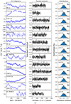 |
Fig. A.1. First column: ‘Raw’ O−C diagrams, namely, without subtracting the quadratic fit performed by Benkő et al. (2019). Note: there are very different vertical scales shown in each panel. Second column: Pseudo-residuals (see formula (9)) associated with the best statistical model. Third column: Normalised distribution of pseudo-residual values (blue histograms) compared to the standard normal distribution (orange curves). In the upper right corner of the panels, the resulting optimal model (M1-M4) is indicated. In the upper left corner, the p-value of the normality test is given. |
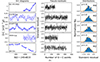 |
Fig. A.1. Continued. |
Appendix B: Statistical fitting of the O−C curves of TESS RRc stars.
 |
Fig. B.1. First column: O−C diagrams calculated from the phase variation functions of Benkő et al. (2023), from which the short-period signals are pre-whitened. Second column: Pseudo-residuals (see formula (9)) associated with the best statistical model. Third column: Normalised distribution of pseudo-residual values (blue histograms) compared to the standard normal distribution (orange curves). In the upper right corner of the panels, the resulting optimal model (M1-M4) is indicated. In the upper left corner, the p-value of the normality test is given. |
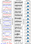 |
Fig. B.1. Continued. |
All Tables
All Figures
|
Fig. 1. Estimations of the phase noise σe from the statistical fit (horizontal scale) with respect to the averaged O−C determination error (vertical scale) for each RRab star in the sample (dots). The solid blue line shows a linear with slope one for comparison. |
| In the text | |
|
Fig. 2. Strength of C2C variation as a function of the main period and some physical parameters for Kepler RRab stars. The stars with no additional frequencies, f1 and f2 frequencies are plotted as filled circles, rectangles and triangles, respectively. The green line shows the significant correlation between period and ση. |
| In the text | |
|
Fig. 3. Segments (of five days) of the residual flux curves of the three brightest TESS RRc stars after the main frequency and its significant harmonics that have been pre-whitened from the data. The relative flux scale is the same for all three stars. There is no detectable structure indicating a C2C variation. |
| In the text | |
|
Fig. 4. Parameter ση characterising the C2C variation for the stars of the RRc sample as a function of the main pulsation period, P1, metallicity, [Fe/H], effective temperature, Teff, and log g. The different symbols show the additional frequency content of the stars (see text for the details). |
| In the text | |
|
Fig. 5. Relation between the fundamentalised period, Pfund, and the effective temperature for the stars in our sample. Red rectangles: RRab stars, blue circles: RRc stars. |
| In the text | |
|
Fig. A.1. First column: ‘Raw’ O−C diagrams, namely, without subtracting the quadratic fit performed by Benkő et al. (2019). Note: there are very different vertical scales shown in each panel. Second column: Pseudo-residuals (see formula (9)) associated with the best statistical model. Third column: Normalised distribution of pseudo-residual values (blue histograms) compared to the standard normal distribution (orange curves). In the upper right corner of the panels, the resulting optimal model (M1-M4) is indicated. In the upper left corner, the p-value of the normality test is given. |
| In the text | |
|
Fig. A.1. Continued. |
| In the text | |
|
Fig. B.1. First column: O−C diagrams calculated from the phase variation functions of Benkő et al. (2023), from which the short-period signals are pre-whitened. Second column: Pseudo-residuals (see formula (9)) associated with the best statistical model. Third column: Normalised distribution of pseudo-residual values (blue histograms) compared to the standard normal distribution (orange curves). In the upper right corner of the panels, the resulting optimal model (M1-M4) is indicated. In the upper left corner, the p-value of the normality test is given. |
| In the text | |
|
Fig. B.1. Continued. |
| In the text | |
Current usage metrics show cumulative count of Article Views (full-text article views including HTML views, PDF and ePub downloads, according to the available data) and Abstracts Views on Vision4Press platform.
Data correspond to usage on the plateform after 2015. The current usage metrics is available 48-96 hours after online publication and is updated daily on week days.
Initial download of the metrics may take a while.