| Issue |
A&A
Volume 696, April 2025
|
|
|---|---|---|
| Article Number | A142 | |
| Number of page(s) | 15 | |
| Section | Cosmology (including clusters of galaxies) | |
| DOI | https://doi.org/10.1051/0004-6361/202453376 | |
| Published online | 11 April 2025 | |
A universal, physically motivated threshold for Hessian-based cosmic web identification: The V-Web case
1
Departamento de Física Teórica, Módulo 15, Facultad de Ciencias, Universidad Autónoma de Madrid, 28049 Madrid, Spain
2
Center for Theoretical Physics, Polish Academy of Sciences, al. Lotników 32/46, Warsaw, Poland
3
Centro de Investigación Avanzada en Física Fundamental (CIAFF), Facultad de Ciencias, Universidad Autónoma de Madrid, 28049 Madrid, Spain
4
International Centre for Radio Astronomy Research, University of Western Australia, 35 Stirling Highway, Crawley, Western Australia 6009, Australia
⋆ Corresponding author; This email address is being protected from spambots. You need JavaScript enabled to view it.
Received:
10
December
2024
Accepted:
24
February
2025
Abstract
Context. The study of large-scale structure benefits from an accurate and robust identification of the cosmic web. Having access to such classifications can facilitate a more complete extraction of cosmological information encoded therein. This information can then help us to improve the mapping and our understanding of galaxy-environment interactions. Classification methods such as T-web and V-web, based on the Hessian matrix, are widely used to single out voids, sheets, filaments, and knots. However, these techniques depend on a threshold parameter whose value is chosen without physical justification and usually rely on a user’s visual impression. Thus, the universality of these results will be limited.
Aims. In this paper, we focus on the V-web method. Our aim is to find a physical motivation for deriving a universal threshold that can be applied across different cosmic scales and epochs.
Methods. V-web classifies the large-scale structure using the eigenvalues of the velocity shear tensor. Using a set of gravity-only simulations, we have introduced a normalization that incorporates the standard deviation of the velocity divergence field, isolating the beyond-Gaussian evolution of cosmic web elements.
Results. In the Zeldovich approximation, the probability of presence of each cosmic web element remains constant at a threshold equal to 0. For the first time, we reveal that this behaviour also holds in the non-linear regime for a normalized positive ‘constant volume threshold’ that depends on both the redshift and the applied smoothing scale. The conservation of volume fractions is valid for the studied redshifts between 0 and 2, regardless of cosmic variance, and it is most precise for intermediate smoothing scales around 3 Mpc/h. The properties of the cosmic web derived using this approach in the V-web align with expectations from other methods, including visual impressions. We provide a general fit formula to compute the constant volume threshold for any standard cosmological simulation, regardless of its specific properties.
Key words: methods: numerical / cosmology: theory / dark matter / large-scale structure of Universe
© The Authors 2025
 Open Access article, published by EDP Sciences, under the terms of the Creative Commons Attribution License (https://creativecommons.org/licenses/by/4.0), which permits unrestricted use, distribution, and reproduction in any medium, provided the original work is properly cited.
This article is published in open access under the Subscribe to Open model. This email address is being protected from spambots. You need JavaScript enabled to view it. to support open access publication.
1. Introduction
It is well understood that dark matter (DM) governs the large-scale distribution of the Universe, as the most gravitationally dominant component of all matter (Planck Collaboration VI 2020). Baryonic matter falls into the gravitational potential of DM and in recent decades, it has been possible to trace its underlying distribution by means of galaxy surveys, ranging from the first small samples from Huchra et al. (1983) and Geller & Huchra (1989) to modern, larger, and deeper catalogs such as Euclid Collaboration (2022). The formation and evolution of this inhomogeneous matter distribution is dominated by the gravitational instability mechanism. The process can be treated analytically using linear and quasi-linear approximations that predict the early stages of DM evolution (Zel’dovich 1970; Peebles 1980). In the subsequent non-linear regime, the DM forms halos by gravitational collapse, where the observed galaxies are located (White & Rees 1978). In turn, these galaxies are immersed in a larger web-like structure called the cosmic web (CW, Bond et al. 1996). Both the properties and evolution of the CW can be studied directly in cosmological simulations and are key to understanding the connection between the DM halos and their environment (e.g. Hahn et al. 2007; Macció et al. 2007; Cautun et al. 2014; Alpaslan et al. 2014; Hellwing et al. 2021; Markos Hunde et al. 2024). In addition, the structure around the galaxies affects their star formation (e.g. Peng et al. 2012; Darvish et al. 2017; Aragon Calvo et al. 2019; Jaber et al. 2024), spin (e.g. Zhang et al. 2015; Pahwa et al. 2016; Ganeshaiah Veena et al. 2019), accretion of satellites (e.g. Knebe et al. 2004; Karachentsev & Kaisina 2019), morphology (e.g. Dressler 1980), and origin (e.g. Codis et al. 2012). Moreover, the CW can shed light on the standard cosmological model (Codis et al. 2018; Bonnaire et al. 2022) and alternatives to general relativity (e.g. Falck et al. 2015; Dome et al. 2023; Gupta et al. 2024).
The classification of the CW elements can be carried out analytically in the linear regime using the Zel’dovich (1970) approximation, which divides the structure into voids, sheets, filaments, and knots, depending on the value of the eigenvalues of the linear deformation tensor. The classification is performed taking into account the sign of the three available eigenvalues and interpreting it as a collapse (‘+’) or expansion (‘−’) in the direction of the corresponding eigenvector. Therefore, the element type can be assigned using only the density field, classifying each region of space into void, sheet, filament, or knot. This strategy has also been used to study the non-linear regime in cosmological simulations using other tensors such as the Hessian of the gravitational potential, which is also known as the tidal field (T-web; Hahn et al. 2007; Aragón-Calvo et al. 2007; Forero-Romero et al. 2009), and the velocity shear tensor (V-web; Hoffman et al. 2012). Other strategies are based on the shear of the Lagrangian displacement field (DIVA; Lavaux & Wandelt 2010) or on the number of orthogonal axes in the Lagrangian phase space sheet (ORIGAMI; Falck et al. 2012). The density field is also widely used in several studies based on segmentation (Spineweb; Aragón-Calvo et al. 2010), finding its topological structures using Morse theory (Colombi et al. 2000), or applying adaptive scaling methods to search for filaments (NEXUS; Cautun et al. 2012). We refer to Libeskind et al. (2017) for a summary and comparison of the CW identification methods.
The benefit of the CW studies using the T-web and V-web (and any of their variations based on Hessian matrix eigenvalues) relies on its easy and straightforward application. The additional advantages consist of their generalization in various types of cosmological simulations and the analytical formulation for T-web in the linear and quasi-linear regime (Ayçoberry et al. 2024). In addition, there is the possibility of applying both methods to observations, using the projected galaxy distribution for T-web (Alonso et al. 2016) and radial peculiar velocities for the V-web (Pomaréde et al. 2017). T-web and V-web are equivalent in the linear regime because at the first perturbative order, the velocity of matter is proportional to its gravitational field.
Although Zeldovich’s approach suggests separating collapse and expansion using the sign of the eigenvalues, subsequent studies in the non-linear regime show better agreement with the distribution of the fields using a positive number between 0 and 1 to separate both situations. Thus, the ‘threshold problem’ arises: the results of T-web and V-web depend on a free parameter, λth, called the threshold, which depends (in most of the cases) on the visual impression of each author. In the literature, several values have been used for the T-web, among which λth = 0 was used by Hahn et al. (2007) as in the linear case, λth = 0.01 by Cui et al. (2017), λth = 0.2 by Libeskind et al. (2014), and λth ∈ [0.2, 0.4] by Forero-Romero et al. (2009), among others. For the V-web, the range λth ∈ [0, 0.6] was used by Pfeifer et al. (2022) and λth = 0.44 by Hoffman et al. (2012) and Libeskind et al. (2014), among others. In many cases, the authors have to study their results based on various thresholds since the conclusions may change with respect to this free parameter. This fact has hindered the use of eigenvalue-based methods to study the time evolution of the CW as well as its generalization across scales, since for each situation, a different threshold would have to be used to visually adjust the matter distribution. It has become an important goal to find a physical motivation to justify a concrete threshold value for T-web and V-web – not only to regularize the results of these methods, but also to build a complete non-linear physical model of the CW without the need for free parameters.
For this purpose, in this paper, we mainly focus on V-web. We study a wide range of possible λth values in a suite of gravity-only ΛCDM simulations with different initial conditions. In each simulation, we make λth proportional to the variance of the velocity field divergence. This normalization allows for a direct comparison of the volume fractions (or probabilities) of each CW element across different redshifts. When analyzing the time evolution, instead of considering each redshift independently, a single threshold value λCV consistently arises across all simulations, at which the fractions of all CW elements remain approximately constant. However, although the volume fraction of each element is conserved, this is not the case for its mass fraction, which shows a time evolution in line with what is expected (see e.g. Cautun et al. 2014; Zhu & Feng 2017). To give a more universal solution that would be applicable to any independent simulation, we provide a fit to obtain λCV depending on the scale and redshift. Testing the fit with an off-set simulation run (with a different baseline cosmology) recovers the expected result, thus confirming the generality of our solution. This fact allows us to analyze the characteristics of the CW and its evolution with V-web, which does not require us to select an arbitrary λth value based on a visual impression. Moreover, it sheds light on possible new physical behaviour in the large-scale distribution of DM related to the conservation of the CW volume fractions.
This paper is organized as follows: In Sect. 2 we summarize the basis of Hessian methods for CW classification and we describe the set of cosmological simulations used in this work. In Sect. 3, we detail how the conservation of volume fractions arises naturally from a suitable eigenvalue normalization and in Sect. 4, we show its consequences in general CW statistics. In Sect. 5, we give indications to the application of the constant volume threshold to generic simulations. In Sect. 6, we offer a brief discussion of the results and some general conclusions.
2. Hessian-based CW classification
By constructing a grid in a gravity-only simulation snapshot, discrete fields located along the volume such as the density contrast, δ(r), gravitational potential, ϕ(r), and velocity, v(r), can be obtained. T-web (Forero-Romero et al. 2009) uses the Hessian of ϕ(r),
 (1)
(1)
to classify each grid cell located in a given position, r, into four types according to how many eigenvalues of the Tij tensor are above a certain threshold, λth. These eigenvalues are labelled according to the order λ1 ≤ λ2 ≤ λ3. If at r no eigenvalue is greater than λth, the cell volume is considered to be a void. If only the largest one, λ1, is above the threshold, the point is classified as a sheet; for the first two, a filament; and for all three, a knot. Intuitively, if we have λi < λth along a certain direction, it indicates expansion in that direction. Conversely, if λi > λth, it signifies compression along that axis. Expansion along all three dimensions implies extensive voids, whereas in contrast, compression along all three directions signifies dense knots. The intermediate situations depend on whether the expansion is in one dimension (filaments) or in two (sheets). Table 1 shows a summary of this classification.
Classification of the CW by eigenvalues used in the T-web and V-web methods.
Alternatively, V-web (Hoffman et al. 2012) uses the eigenvalues of the velocity shear tensor defined as
 (2)
(2)
where the Hubble parameter H(z) scales the tensor for each redshift and makes it dimensionless (Libeskind et al. 2014). The ‘−’ sign included in the definition (2) makes the collapse and expansion conditions the same as in Table 1. For each grid cell, we can further take the trace of the velocity shear tensor tr(Σ), resulting in the velocity divergence field θ(z):
 (3)
(3)
Prior to diagonalization, a smoothing is performed to mitigate the effects of the grid discretization. For this purpose, we use a Gaussian kernel of the form:
 (4)
(4)
where Rs is a co-moving smoothing scale in Mpc/h units, also referred to as smoothing length. This distance has to be greater than twice the grid spacing used, since at smaller distances, the convolution would not affect contiguous cells. It should also not exceed half the side of the simulated box.
We can calculate the standard deviation of the divergence field ⟨θ2⟩1/2 = σθ, with a value that is lower for early times with a homogeneous velocity distribution and higher for late times involving larger non-Gaussianities. This relationship follows from ∇ ⋅ v ∝ −δ in the linear regime (Peebles 1980; Chodorowski 1997). Similarly, σθ is smaller at higher smoothing lengths, Rs, since in the linear regime, we have σθ ∝ σδ and
 (5)
(5)
where P(k) is the matter power spectrum. If we assume that the contrast density field δ is Gaussian, then θ is also Gaussian and therefore we can compute the joint probability of the eigenvalues of Σij using Doroshkevich’s formula (Doroshkevich 1970):
![Mathematical equation: $$ \begin{aligned} p(\lambda _{1},\lambda _{2},\lambda _{3})&= \frac{3375}{8\sqrt{5}\pi \sigma _{\theta }^{6}}\exp \bigg [-\frac{3}{\sigma _{\theta }^{2}}\left(\sum _{i=1}^{3}\lambda _{i}\right)^2 \nonumber \\&+\frac{15}{2\sigma _{\theta }^{2}}\sum _{i>j}\lambda _{i}\lambda _{j}\bigg ]\, \vert \Pi _{i >j}(\lambda _{i}-\lambda _{j})\vert .\end{aligned} $$](/articles/aa/full_html/2025/04/aa53376-24/aa53376-24-eq6.gif) (6)
(6)
Therefore, the probability, PE, of having an element type E in the V-web classification in the Gaussian case depends on the joint probability given by Eq. (6) and the condition determined for each element in Table 1 (Ayçoberry et al. 2024):
 (7)
(7)
where CE is the function that contains the Boolean condition of each element, being 1 if it is satisfied or 0 if not. The integral PE depends not only on the threshold, but also on parameters such as redshift, smoothing length, and cosmology due to the presence of σθ in Eq. (6). The equivalent of the probability of an environment E in cosmological simulations is the volume fraction  , which is obtained by summing the volume occupied by element E and dividing by the total volume of the box. Under periodic boundary conditions,
  . To investigate the non-Gaussian regime where this equality no longer applies, we generated a set of cosmological simulations designed to accurately reproduce the CW at low redshift.
We employed the COmoving Lagrangian Accelerator (COLA) method (Tassev et al. 2013) to obtain our set of N-body simulations. The parallel implementation of the COLA algorithm called L-PICOLA (see Howlett et al. 2015) allows us to run large simulations at a reduced computational cost, with the trade-off of limited spatial and temporal resolution. Specifically, we used a publicly available optimized branch of the L-PICOLA family, the MG-COLA, developed by Winther et al. (2017). COLA achieves the significant speed-up mostly at the expense of the accuracy of DM halo properties. For example, the method is known to weakly bias the resulting halo velocities. This bias is small (up to ∼5% for our case) and mainly concerns the small-scale halo velocity field (see more in Munari et al. 2017). However, the COLA simulations convergence to the full N-body results is very good for the large-scale smooth density and velocity fields for the scales and epoch we consider in this paper. We used a set of ten gravity-only simulations in MG-COLA with a box size of L = 250 Mpc/h and with Np = 5123 particles each representing mp = 8.6 × 10⁹ M⊙/h matter element, under periodical boundary conditions. All simulations have different initial phases. To ensure a sufficient level of accuracy for the COLA method at small scales, we used a total of 15 time steps from the initial conditions (three steps linearly distributed between the redshifts z = 0, 0.3, 0.5, 1, 2, 10). The cosmological parameters we used are: Ωm = 0.267, Ωb = 0.049, h = 0.71, σ8 = 0.8, and n = 0.966.
3. CW evolution
The typical way V-web and T-web are applied is to perform a static classification at a given redshift, using a preselected threshold, λth, chosen by a visual inspection. This approach prohibits both methods from being used for a consistent analysis of the CW evolution. We show that accounting for the time evolution of the large-scale cosmic fields, including their associated Hessian eigenvalues, enables the determination of a unique, time-dependent mapping for the optimal (and natural) V-web threshold, λCV. We find that this mapping is robust and universal and can be used for consistent V-web components identification across redshift, simulations, and cosmologies.
3.1. The threshold problem
An example of an N-body simulation of our set where V-web was applied is shown in Fig. 1. Using a smoothing length of Rs = 1 Mpc/h, the density and velocity fields are computed on a Ng = 5123 grid, as well as the classification of the CW elements according to the value of the eigenvalues of Eq. (2). Panels a and b contain the logarithm of the DM density distribution log10(δ + 1) computed on a ∼1.5 Mpc/h thick slice (or three times the grid spacing), for z = 2 and z = 0, respectively. For both redshifts, it is possible to distinguish zones with higher matter density, which usually end up forming galaxy clusters, and zones with lower density that tend to empty as the matter flows towards the regions with higher concentrations. It can be noted that the CW must be mostly occupied by voids, with the denser knot-like zones bound by thin sheets and filaments.
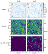 |
Fig. 1. Density and V-web classification of a gravity-only ΛCDM simulation. The cube is divided into a Ng = 5123 cells grid on which both the density and the eigenvalues of the shear velocity tensor have been calculated, applying a smoothing of Rs = 1 Mpc/h. Panels a and b show the logarithm of the DM density at redshifts 2 and 0 respectively (in a slice that has a thickness of ∼1.5 Mpc/h). Panels c and d contain, for the previous redshifts, the classification into CW elements performed by the V-web method for an λth = 0 (in a middle slice that is one grid cell thick). Panels e and f contain the same as the previous two, but for the λth = 0.44 proposed by Hoffman et al. (2012). |
The classification made by the V-web in the slice formed by the cells in the middle is shown in the rest of the panels. For c and d, where we have applied a threshold λth = 0, there is an excess of structure that leaves voids as a minority element compared to filaments and sheets. This feature contradicts the primary observations that predict a Universe mostly full of voids (see Gregory & Thompson 1978; Jôeveer et al. 1978; Tully & Fisher 1978, for first detections), making use of λth = 0 unfavorable. In panels e and f, we have applied λth = 0.44 motivated by Hoffman et al. (2012), which significantly improves the closeness to the visual impression at z = 0. However, a constant threshold cannot account for the non-linear evolution of the eigenvalues λi, as it neglects the fact that these values are generally closer to 0 in a younger Universe with more homogeneous density and velocity fields. Consequently, it results in an overly high threshold for z = 2, leading to a scenario, where almost the entire simulated space is classified as a void, thereby losing the structural details.
Table 2 contains the volume fractions computed for the simulation shown in Fig. 1. The scarce presence of voids in the case of λth = 0 occurs because they occupy less than 15% of the total volume at all times, as opposed to filaments and sheets, which occupy more than 80% of the space. In contrast, when λth = 0.44 is applied at z = 2, most of the λi values fall below λth, resulting in over 99% for the void fraction. The threshold problem extends not only to the redshift evolution, but also to the smoothing scales used, as we have to adjust the λth value when the scale is changed. This issue prevents us from using V-web (and T-web) in an automated and self-consistent way.
3.2. The dependence of the volume fractions evolution on the threshold
Since the volume fractions can also be understood in the probabilistic sense, we present the values of PE defined in (7) for the selected thresholds in parentheses in Table 2. Since Eq. (6) only works for Gaussian fields, the linear result can only give a slight approximation of the values obtained for the simulation. We note that for the value suggested by Zeldovich’s approximation of λth = 0, the linear volume fractions do not change along the redshift; thus, this is the only value for which this conservation is satisfied.
If we slightly increase the value of λth above 0, it is more likely that λ2 and λ3 are smaller than the threshold, so we expect an increase in the volume fraction of both the sheets and voids. If we continue to increase λth, there is a certain moment when λth is above all λi so the fraction of voids is greater than that of the sheets. Finally, for a λth > λ1 ≥ λ2 ≥ λ3 case, the voids occupy all of the space. The left panel of Fig. 2 shows the evolution of the V-web volume fraction fv(z, λth) at Rs = 3 Mpc/h for the simulation presented in the previous figure. For λth > 0, the behaviour described for sheets and voids can be observed. In the case of λth < 0, a similar behaviour is seen for filaments and knots.
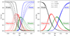 |
Fig. 2. Volume fractions of the CW elements obtained with V-web from a simulation shown in Fig. 1. The left panel show the results using the same threshold for all redshifts, while in the right panels, Eq. (8) has been used to normalize λth. The applied smoothing length is Rs = 3 Mpc/h. |
In the left panel of Fig. 2, we can see that the solid lines representing z = 2 are closer to λth = 0 than the other redshifts because the distribution of eigenvalues is more restricted for a younger (i.e. more homogeneous) Universe. As the non-linear evolution progresses, the variance of the velocity field grows, and the eigenvalues can take a larger range of values. This causes the volume fractions to stretch at lower redshifts, extending their presence to threshold values farther from zero. We can normalize λth with the variance of the velocity divergence σθ(z) to partially account for this effect. Therefore, we studied the volume fractions using a normalized  defined as:
 (8)
(8)
This normalization allows us to cancel the linear evolution of the CW because using  as a threshold in the V-web is equivalent to multiplying λi by the factor σθ(z)/σθ0 in the conditions of Table 1. We note that although we chose z = 0 as the reference redshift, picking another value in the re-scaling would not change the results since the threshold
  applied to V-web would always be the same (see Appendix C for proof). The above transformation applied to Doroshkevich’s formula (6) and to the differentials of Eq. (7) cancels all σθ(z) terms of the PE function and replaces them with σθ0, which implies the loss of time dependence and
 (9)
(9)
for a Gaussian case. Thus, we can expect similar (but not identical) behaviour for the volume fractions, fv, of the CW fields extracted from cosmological simulations.
In the following, when we consider z > 0 snapshots, we apply  as a threshold in the V-web to extract volume fractions or other quantities. To compare properties obtained using different
  , we use λth common to all redshifts by Eq. (8). The right panel of Fig. 2 contains the volume fractions for the threshold values after normalization (8). The x-axis represents λth; therefore, for each snapshot at redshift, z, the volume fraction,
  is obtained using the
  threshold in V-web. This strategy reduces the difference between the redshifts and brings all the volume fractions in each element closer to those obtained at z = 0. However, there are still small differences depending on z and λth, stemming from non-linear gravitational evolution that drives the cosmic fields away from a Gaussian distribution for late times and/or small scales.
This can be better seen in Fig. 3, where we show the difference between the volume fractions at the present time fv0(λth)≡fv(z = 0, λth) minus the volume fractions at the four other redshifts, for the same initial conditions and smoothing length as in Fig. 2. At the extreme λth, the differences tend to be zero for all elements because, at all redshifts, there is a dominance of knots at λth < 0, and the dominance of voids at λth > 0. However, the intermediate values contain information on how the volume fractions vary over time in mixed regimes with all CW elements present in the Universe, so we restricted the analysis to thresholds where no single element exceeds a volume fraction of 0.99.
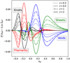 |
Fig. 3. Evolution of the difference in volume fractions after λth normalization defined in Eq. (8). Each line is the volume fraction at z = 0 minus the volume fraction at other redshifts (differentiated with the type of pattern), as a function of λth. The colour code, simulation, and RS value is the same as the one used in Fig. 2. The magenta circle marks the constant volume threshold λCV in which the volume fractions of each element become approximately constant over time. |
In Fig. 3, we note that there is a special λth value that (despite it being intermediate between the two extreme situations) cancels out the volume differences at this value for all redshifts and CW elements. Indicated by the magenta circle, the volume fraction differences of all CW elements reach a minimum in this ‘constant volume’ threshold, λCV. This means that if we choose as threshold the related value  for the V-web, we always have approximately the same volume fractions for z and z = 0. This effect occurs because the curve for voids, filaments, and sheets changes sign at this λCV. Regarding the knot line, it appears that it tends to very low values from λth less than λCV to the extreme dominated by voids. The same behaviour was found for Rs between 1 and 6.5 Mpc/h, but with different values of λCV depending on the case.
We note that λCV may be redshift-dependent because its value differs slightly depending on the z at which the volume fractions are computed. To locate λCV in a multitude of different simulations and redshifts, we define the function S as:
 (10)
(10)
Thus, using the sum of the differences for all CW elements.
Function S is shown in Fig. 4 for different redshifts. The threshold λCV, marked with a magenta circle, corresponds to a local minimum of S in the intermediate zone between extremes. This minimum also appears for the other redshifts in a similar threshold. Given any gravity-only simulation, it is possible to find an approximate value of λCV by first calculating its fv with threshold  as a function of λth for different redshifts, and then computing the local minimum of S between 0 and 1. Once λCV is found for a given z, it is possible to perform a V-web analysis by applying λCV to the z = 0 snapshot and
  for the snapshot at a redshift, z.
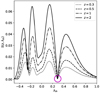 |
Fig. 4. Function S defined in Eq. (10) calculated for the simulation of the previous figures (Rs = 3 Mpc/h). The magenta circle marks S(λCV). |
We have used the same methodology for ten gravity-only ΛCDM simulations (described in Sect. 2), where the V-web was applied on a grid of 5123 cells. The only difference between the simulations is the random seed used to pick the phases in the initial conditions. In all of them, we have found a conservation of the volume fractions at a specific λCV, similar to the behaviour seen in Fig. 3, where the differences of each CW element tend to 0 at a similar threshold value.
3.3. Constant volume threshold, λCV
By repeating the entire process described in the previous subsection for all simulations in the set, Fig. 5 presents the mean λCV as a solid line across different redshifts for a specific Rs. The shaded regions with fainter colours represent the standard deviation σ for the set of simulations. We note that the mean value of λCV shows a slight variation with redshift. However, it exhibits a clear dependence on the Rs used to compute the V-web eigenvalues.
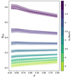 |
Fig. 5. Mean of λCV computed using the minimum of the function S in each simulation of our set, shown as solid lines. The dashed lines correspond to the fit defined in Eq. (13), as explained in Sect. 5.1. The different colours correspond to the smoothing length used in the analysis, with the shading indicating the σ region of the set. |
Figure 6 shows the mean value of λCV as a function of Rs, highlighting its decrease with increasing smoothing length. For a large value of Rs, the eigenvalues tend to have a Gaussian distribution more centered on 0, so λCV tends to the same central value (i.e. λCV → 0). We have not considered Rs larger than 6.5 Mpc/h, since from this value, the voids satisfy  ; thus the value of
  would be left out of the delimited intermediate regime. On the other hand, the resolution of the grid limits the smoothing length to:
 (11)
(11)
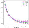 |
Fig. 6. Mean of λCV for different redshifts, as a function of the smoothing length, Rs. The error bars indicate the σ region of the set. |
where L is the box size and Ng is the number of cells per grid dimension.
Just as the volume fractions are not exactly conserved because S(z, λCV) is never exactly 0, neither is the value of λCV exactly the same for different redshifts. This is more evident from Fig. 5 for Rs = 1 Mpc/h, where λCV seems to tend to smaller values for higher z. On the contrary, for higher values of Rs the constant volume threshold appears to increase slightly with z. Details on the accuracy of the volume fraction conservation as a function of z and Rs are given in Appendix A. In the next section, we examine in detail how this approximate conservation influences the CW classification and volume fractions across different scales and redshifts.
4. CW at a constant volume fraction
Taking into account the evolution of the CW enables the selection of a specific threshold to be used with V-web for analyzing the spatial distribution of each element. It is crucial to assess whether this classification is consistent with the fundamental properties expected in the CW.
4.1. The evolution of the cosmic web at λCV
A first intuitive approach is to visually inspect how V-web classifies the CW elements when the threshold is  . Figure 7 shows this classification for the same simulation as shown in Fig. 1. This time, we have shown the case for constant volume threshold in three different smoothing lengths. The visual effect of using different Rs values is the level of small scale detail we can achieve. For all three cases we see a clear evolution of the CW components, from more homogeneous structures at z = 2 to formations with more complexity at z = 0. We note that although each region naturally changes type over time, the use of λCV ensures that the volume fraction remains nearly constant.
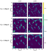 |
Fig. 7. V-web classification of the simulation shown in Fig. 1, applying in this case the threshold |

In the particular case of Rs = 3 Mpc/h, it is remarkable how the sheets subdivide with time, going from a homogeneous distribution at z = 2, to increasing number of connections at the present time. Also, as for the filaments, it seems that with time new connections are generated between different knots that allow for the exchange of matter between more regions. This is repeated for smaller scales at Rs = 1 Mpc/h and for larger scales at Rs = 5 Mpc/h. In some cases, in the three smoothing lengths the knots and filaments seem to appear and disappear erratically between one time or another. However, this can be explained by the fact that due to their small size they are sensitive to peculiar movements, which can cause them to be lost or included in the two-dimensional slice we use to represent the CW. This effect has to be taken into account also for the other elements, thus limiting the ability of the 2D projections to diagnose the evolutionary behaviour. In the following sections, we deal with global quantities of the simulations such as the volume fraction (Sect. 4.2) or mass fraction (Appendix B).
4.2. Volume fractions at λCV
The volume fractions calculated for Fig. 7 using the constant volume threshold  are listed in Table 3. Note the precise conservation of volume fractions for the case Rs = 3 Mpc/h between z = 2 and z = 0 (satisfied to three significant digits in voids, sheets and knots). For the values Rs = 1 Mpc/h and Rs = 5 Mpc/h, the volume fractions vary slightly from one redshift to another, especially for elements with less statistical presence such as filaments and knots. From Table 3 it can also be seen that the volume fractions vary with respect to the Rs used at the same z.
The analysis for the set of ten simulations is presented in Fig. 8, showing the volume fractions calculated in the constant volume threshold (we leave the discussion of mass fractions for Appendix B). For Rs values lower than ∼3 Mpc/h, we see that void volume fraction and Rs are inversely correlated. At larger values of Rs, the correlation is reversed and there is a greater presence of voids given a larger smoothing. This trend seems to be inverted for the other elements
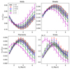 |
Fig. 8. Mean volume fractions for different CW elements computed using |

We can understand this behaviour by looking at the dominant element. At first glance, Fig. 7 shows that below Rs ∼ 3 Mpc/h, the amount of space occupied by voids increases as Rs decreases. This is due to the fact that as we increase the complexity of the structure, the filaments, sheets, and knots are subdivided into finer and smaller parts separated from each other by voids. If we assume a Rs tending to 0, the field structure disappear except for the small regions of DM halos, which are stationary under eigenvalue formalism. In this case, we see a dominance with respect to voids, since all halos and nodes are contracted effectively to volume-less points. If we increase in Rs above ∼3 Mpc/h, the voids tend to increase, but for another reason. As the variance of the Gaussian window function increases, the Universe tends to become more and more homogeneous and inhomogeneities tend to be smaller. Since the perturbations are where the sheets, filaments, and knots originate, this implies an increase of voids against them.
We note that in Fig. 8 the case for z = 0 has been included, but in principle it is not possible to define  since we need to use a non-zero redshift in the function S(z, λth). However, as λCV shows a slight variation with time, we can consider that
  for a z close to 0 can be valid also for z = 0, thus drawing the volume fraction for this redshift from the
  . The results in this extrapolation have very similar values for voids and sheets, although they differ for more sensitive elements such as filaments and knots. Considering all redshifts, the volume fractions are observed to be of similar order of magnitude, although they exhibit slight variations across different z values. This is due to the fact that volume conservation is not perfect and λCV is not strictly constant over time (see Appendix A). In fact, the regime where λCV is most stable over time (between 2 and 4 Mpc/h depending on the element) is also the regime in which appears the best volume conservation, with there being a crossover of all lines at those values of Rs. This effect indicates that both the volume fraction and λCV conservation tend to occur more accurately over a range of intermediate values of the smoothing length. Since the Gaussian and top-hat smoothing windows also have no fixed choice in the standard analysis, the logic of the constant volume threshold may also help resolve this ambiguity.
If we compare the volume fractions from the V-web using λCV with those obtained by other widely used techniques, such as Nexus+ (Cautun et al. 2014), we get very similar results. For z = 0, the mean fractions for smoothing lengths where conservation is more accurate (Rs = 3 Mpc/h) are [0.77, 0.20, 0.031,0.0015] for voids, sheets, filaments and knots, respectively. For Nexus+, these values are [0.77,0.18,0.06,< 0.001], with both methodologies differing mainly in the most sensitive elements such as filaments and knots.
5. Application of the λCV threshold to generic N-body simulations
The objective of this section is to provide a generic fit of λCV that can be used in different types of cosmological simulations that are not necessarily restricted to the characteristics of the set used in this work. The idea is to give the community an easy way to obtain the value of λCV(z, Rs) for a generic cosmological simulation based only on the redshift and Gaussian smoothing scale specified. An example application is presented in Sect. 5.2, applying the fitting function obtained as the V-web threshold in a full N-body simulation with different initial conditions, box size, number of particles, and cosmology than those used in the main set.
5.1. Approximating the dependence on scale and redshift
Given the reduced redshift dependence of λCV, we approximate  for each Rs to a line of slope a and vertical intercept b:
 (12)
(12)
where a and b depend on the Rs used. The function a quantifies the deviation from the constant value in z, being negative for small Rs and positive for high Rs. Function b contains the general behaviour of λCV as a function of scale. Figure 9 shows the values of a (left panel) and b (right panel) measured for the main set of simulations, as well as the non-linear least squares fit applied. An exponential function can be used to approximate the dependence of both parameters on Rs, so the fit equations give the following results:
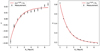 |
Fig. 9. Parameters a and b defined in Eq. (12) and measured by least squares applied to each value of Rs used to obtain λCV in the MG-COLA set of simulations. The error bars (small in the right panel) are given by the square root of the diagonal elements in the covariance matrix. Both parameters have been approximated to an exponential type function plotted in red, whose constants are given in Table 4. The result of the approximation is a fit |

 (13)
(13)
 (14)
(14)
with the parameters values obtained from our set and given in Table 4. The standard deviation errors of the fit parameters are calculated by the square root of the diagonal of the covariance matrix.  is represented by dashed lines in Fig. 5, confirming that the fit falls within the σ cosmic variance at all represented Rs values. The procedure for using the fit is as follows: first, substitute in Eqs. (13) and (14) the Rs used, and input the redshift into Eq. (12) to get
  . Next, since
  has the role of λth in Eq. (8), compute σθ0 and σθ(z) to obtain
  . This is the threshold to be used in the V-web for the snapshot at redshift, z. We note that if z = 0, then the second step is not necessary.
For example, to determine the threshold for Rs = 4 Mpc/h and z = 0 it is sufficient to calculate b(Rs) from Eq. (14), yielding  . If, instead, z = 2 is considered for same Rs, the procedure requires calculating a(Rs) from Eq. (13), followed by applying the re-scaling (8) to the resulting
  . Applying this approach to the simulation from our set shown in Fig. 1, where σθ0 = 0.30 and σθ(z = 2) = 0.10 for Rs = 4 Mpc/h, the resulting threshold for V-web at snapshot z = 2 is
  .
.
5.2. λCV in a N-body simulation outside the set
We have reproduced the whole process of λCV calculation for an example full N-body simulation. Since the normalization of Eq. (7) deals with σθ ratios, the dependence of λCV on similar cosmological parameters is very small and its value can be approximated by  for off-set ΛCDM simulations. This is because the first term of the Taylor expansion of the velocity field variance captures the main bulk effect of varying cosmology (see e.g. Nusser & Colberg 1998).
As a working example of the N-body simulation, we have taken a run done with Gadget-2 code (Springel 2005) with a use of Np = 12803 particles each representing mp = 1.8 × 10¹⁰ M⊙/h matter element, placed in a periodic box of L = 800 Mpc/h (Hellwing et al. 2017). The cosmological parameters used to generate the initial conditions and fix the expansion history were that of the 7-year data release of the WMAP mission (Komatsu et al. 2011). Figure 10 shows the volume fraction differences for the Gadget simulation in a similar way to that drawn in Fig. 3 for a simulation from the MG-COLA set. In the first three panels, a particular redshift is depicted and for each one, the corresponding  is represented by the vertical black line (whose thickness matches three times the propagated uncertainty, σfit). It can be seen that the volume fractions of all elements remain constant at a specific threshold value, confirming the existence of the constant volume threshold in the off-set simulation. The right panel shows with red stars the value of λCV calculated for the N-body simulation using the standard procedure of minimizing the S(z, λth) function. This falls within the values expected by
  for the represented redshifts.
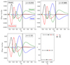 |
Fig. 10. Differences in volume fractions at different redshifts (shown in the first three panels) calculated for an off-set Gadget simulation. The constant volume threshold phenomenon appears for all classified elements despite the fact that the cosmology, box size, initial conditions, and code are different from those of the MG-COLA set used in the rest of the work. The black vertical area shows the calculated range for |


6. Concluding remarks
The study of the cosmic web is essential for a comprehensive understanding of large-scale structure, so its analysis requires a consistent classification based upon solid physical principles. Among the various existing techniques for identifying the structures that make up the cosmic web, Hessian matrix-based methods stand out for their simplicity, theoretical motivation, and potential applicability to observations. These methods allow for the identification of voids, sheets, filaments, and knots, depending on the principal axes of collapse of the gravitational potential (T-web) or the velocity field (V-web). However, both classifications rely on a threshold, λth, that has not been assigned with a physical value and has so far been chosen primarily through visual inspection.
In this work, we address this problem for the case of the V-web classification by using the statistical principles governing Gaussian eigenvalues (e.g. Doroshkevich’s formalism), focusing our analysis on the probability of each cosmic web element’s presence quantified by its volume fraction. To analyze the non-linear evolution we use a set of ten ΛCDM simulations generated by MG-COLA under different initial conditions. In this set, the V-web method is applied using a threshold normalized by the standard deviation of the velocity divergence field. As shown in Fig. 3, this approach reveals a unique positive threshold at which all volume fractions remain constant over time. Figures 5 and 6 indicate that this constant volume threshold λCV depends on scale but shows little variation with cosmic variance or redshift. The resulting classification (Fig. 1) agrees with the choice by visual inspection reported in previous works, such as Hoffman et al. (2012). Moreover, the volume fractions obtained using λCV at scales close to Rs = 3 Mpc/h, where conservation is most precise, are consistent with those predicted by other methods, such as Nexus+ (Cautun et al. 2014). Similarly, the evolution of the mass distribution across different cosmic web elements aligns with previous findings.
As an alternative to the arbitrary threshold in the V-web method, we provide a fit for λCV. This fit depends on the applied Gaussian smoothing length, Rs, and the redshift, z, for which V-web is used. If z = 0, then the threshold  that keeps the volume constant is equal to the function b(Rs) of Eq. (14). If z > 0, then we must also calculate the function a(Rs) of Eq. (13) and substitute both in Eq. (12) to obtain
  , to finally calculate the V-web threshold by means of the re-scaling defined by Eq. (8). Finally, we test the universality of this fit using a Gadget simulation with characteristics distinct from those of the MG-COLA set. As shown in Fig. 10, the simulation outside the set demonstrates volume fraction conservation that aligns with
  .
.
The clear manifestation of λCV motivates a universal threshold for the V-web, which would be both physically motivated and independent of user choice. Our results hint also towards a new fundamental physical behaviour in this type of Hessian classification. The origin of the volume conservation observed in this work is still unknown, although there are several possible explanations. Some studies of the topological properties (the Betti numbers and the Genus) show that these features are fixed for any given Gaussian field (e.g. Pranav et al. 2016; Wilding et al. 2021). This indicates that a gravitational evolution up to a weakly non-linear regime should not drastically change the underlying topology, so we can also expect that a similar conservation could be present for the V-web elements. Other authors have suggested that a more realistic description of the protohalo boundary is one that minimizes the enclosed energy while preserving the volume (Musso & Sheth 2023) and this concept can be studied in the cosmic web by means of the energy shear tensor (Musso et al. 2024).
The next step will be the construction of an analytical framework based on the quasi-linear approximation that can be used to explain the conservation of probability in the V-web. In addition, we will test whether this behaviour appears only for ΛCDM or holds also for significant changes to the cosmological parameters or even beyond-ΛCDM models. Both perspectives will allow us to get closer to a general theory of the cosmic web, which has yet to be constructed, and to get a deeper understanding of the relationships between dark matter halos and large-scale structure.
Acknowledgments
All authors thank the referee for their constructive comments that helped to improve the paper. The authors are grateful for inspiring discussion and comments from Adi Nusser and Mariana Bravo Jaber, received at early stage of this work. EO thanks Yehuda Hoffman for his advice and Anastasia Hrabarchuk for her insistence. EO and AK are supported by the Ministerio de Ciencia e Innovación (MICINN) under research grant PID2021-122603NB-C21. EO received predoctoral fellowship from MICINN (FPI program, Ref. PRE2022-102254). AK further thanks Portishead for dummy. WAH acknowledges the support from the research projects funded by the National Science Center, Poland, under agreement number #2018/30/E/ST9/00698 and #2018/31/G/ST9/03388.
References
- Alonso, D., Hadzhiyska, B., & Strauss, M. A. 2016, MNRAS, 460, 256 [NASA ADS] [CrossRef] [Google Scholar]
- Alpaslan, M., Robotham, A. S. G., Obreschkow, D., et al. 2014, MNRAS, 440, L106 [Google Scholar]
- Aragón-Calvo, M. A., Jones, B. J. T., van de Weygaert, R., & van der Hulst, J. M. 2007, A&A, 474, 315 [NASA ADS] [CrossRef] [EDP Sciences] [Google Scholar]
- Aragón-Calvo, M. A., Platen, E., van de Weygaert, R., & Szalay, A. S. 2010, ApJ, 723, 364 [Google Scholar]
- Aragon Calvo, M. A., Neyrinck, M. C., & Silk, J. 2019, The Open Journal of Astrophysics, 2, 7 [Google Scholar]
- Ayçoberry, E., Barthelemy, A., & Codis, S. 2024, A&A, 686, A276 [NASA ADS] [CrossRef] [EDP Sciences] [Google Scholar]
- Bond, J. R., Kofman, L., & Pogosyan, D. 1996, Nature, 380, 603 [NASA ADS] [CrossRef] [Google Scholar]
- Bonnaire, T., Aghanim, N., Kuruvilla, J., & Decelle, A. 2022, A&A, 661, A146 [NASA ADS] [CrossRef] [EDP Sciences] [Google Scholar]
- Cautun, M., van de Weygaert, R., & Jones, B. J. T. 2012, MNRAS, 429, 1286 [Google Scholar]
- Cautun, M., van de Weygaert, R., Jones, B. J. T., & Frenk, C. S. 2014, MNRAS, 441, 2923 [Google Scholar]
- Chodorowski, M. J. 1997, MNRAS, 292, 695 [NASA ADS] [CrossRef] [Google Scholar]
- Codis, S., Pichon, C., Devriendt, J., et al. 2012, MNRAS, 427, 3320 [NASA ADS] [CrossRef] [Google Scholar]
- Codis, S., Pogosyan, D., & Pichon, C. 2018, MNRAS, 479, 973 [Google Scholar]
- Colombi, S., Pogosyan, D., & Souradeep, T. 2000, Phys. Rev. Lett., 85, 5515 [Google Scholar]
- Cui, W., Knebe, A., Yepes, G., et al. 2017, MNRAS, 473, 68 [Google Scholar]
- Darvish, B., Mobasher, B., Martin, D. C., et al. 2017, ApJ, 837, 16 [Google Scholar]
- Dome, T., Fialkov, A., Sartorio, N., & Mocz, P. 2023, MNRAS, 525, 348 [NASA ADS] [CrossRef] [Google Scholar]
- Doroshkevich, A. G. 1970, Astrophysics, 6, 320 [Google Scholar]
- Dressler, A. 1980, ApJ, 236, 351 [Google Scholar]
- Euclid Collaboration (Scaramella, R., et al.) 2022, A&A, 662, A112 [NASA ADS] [CrossRef] [EDP Sciences] [Google Scholar]
- Falck, B. L., Neyrinck, M. C., & Szalay, A. S. 2012, ApJ, 754, 126 [Google Scholar]
- Falck, B., Koyama, K., & Zhao, G.-B. 2015, JCAP, 2015, 049 [CrossRef] [Google Scholar]
- Forero-Romero, J. E., Hoffman, Y., Gottlöber, S., Klypin, A., & Yepes, G. 2009, MNRAS, 396, 1815 [Google Scholar]
- Ganeshaiah Veena, P., Cautun, M., Tempel, E., van de Weygaert, R., & Frenk, C. S. 2019, MNRAS, 487, 1607 [NASA ADS] [CrossRef] [Google Scholar]
- Geller, M. J., & Huchra, J. P. 1989, Science, 246, 897 [NASA ADS] [CrossRef] [Google Scholar]
- Gregory, S. A., & Thompson, L. A. 1978, ApJ, 222, 784 [NASA ADS] [CrossRef] [Google Scholar]
- Gupta, S., Pfeifer, S., Ganeshaiah Veena, P., & Hellwing, W. A. 2024, Phys. Rev. D, 110, 083520 [Google Scholar]
- Hahn, O., Porciani, C., Carollo, C. M., & Dekel, A. 2007, MNRAS, 375, 489 [NASA ADS] [CrossRef] [Google Scholar]
- Hellwing, W. A., Nusser, A., Feix, M., & Bilicki, M. 2017, MNRAS, 467, 2787 [NASA ADS] [Google Scholar]
- Hellwing, W. A., Cautun, M., van de Weygaert, R., & Jones, B. T. 2021, Phys. Rev. D, 103, 063517 [NASA ADS] [CrossRef] [Google Scholar]
- Hoffman, Y., Metuki, O., Yepes, G., et al. 2012, MNRAS, 425, 2049 [Google Scholar]
- Howlett, C., Manera, M., & Percival, W. J. 2015, Astron. Comput., 12, 109 [NASA ADS] [CrossRef] [Google Scholar]
- Huchra, J., Davis, M., Latham, D., & Tonry, J. 1983, ApJS, 52, 89 [NASA ADS] [CrossRef] [Google Scholar]
- Jaber, M., Peper, M., Hellwing, W. A., Aragón-Calvo, M. A., & Valenzuela, O. 2024, MNRAS, 527, 4087 [Google Scholar]
- Jôeveer, M., Einasto, J., & Tago, E. 1978, MNRAS, 185, 357 [NASA ADS] [CrossRef] [Google Scholar]
- Karachentsev, I. D., & Kaisina, E. I. 2019, Astrophysical Bulletin, 74, 111 [NASA ADS] [CrossRef] [Google Scholar]
- Knebe, A., Gill, S. P. D., & Gibson, B. K. 2004, PASA, 21, 216 [Google Scholar]
- Komatsu, E., Smith, K. M., Dunkley, J., et al. 2011, ApJS, 192, 18 [Google Scholar]
- Lavaux, G., & Wandelt, B. D. 2010, MNRAS, 403, 1392 [NASA ADS] [CrossRef] [Google Scholar]
- Libeskind, N. I., Hoffman, Y., & Gottlöber, S. 2014, MNRAS, 441, 1974 [CrossRef] [Google Scholar]
- Libeskind, N. I., van de Weygaert, R., Cautun, M., et al. 2017, MNRAS, 473, 1195 [Google Scholar]
- Macció, A. V., Dutton, A. A., Van Den Bosch, F. C., et al. 2007, MNRAS, 378, 55 [NASA ADS] [CrossRef] [Google Scholar]
- Markos Hunde, F., Newton, O., Hellwing, W. A., Bilicki, M., & Naidoo, K. 2024, A&A, submitted [arXiv:2409.09226] [Google Scholar]
- Munari, E., Monaco, P., Koda, J., et al. 2017, JCAP, 7, 050 [CrossRef] [Google Scholar]
- Musso, M., & Sheth, R. K. 2023, MNRAS, 523, L4 [NASA ADS] [CrossRef] [Google Scholar]
- Musso, M., Despali, G., & Sheth, R. K. 2024, A&A, 690, A214 [NASA ADS] [CrossRef] [EDP Sciences] [Google Scholar]
- Nusser, A., & Colberg, J. M. 1998, MNRAS, 294, 457 [NASA ADS] [CrossRef] [Google Scholar]
- Pahwa, I., Libeskind, N. I., Tempel, E., et al. 2016, MNRAS, 457, 695 [NASA ADS] [CrossRef] [Google Scholar]
- Peebles, P. J. E. 1980, The Large-scale Structure of the Universe (Princeton: Princeton University Press) [Google Scholar]
- Peng, Y.-J., Lilly, S. J., Renzini, A., & Carollo, M. 2012, ApJ, 757, 4 [NASA ADS] [CrossRef] [Google Scholar]
- Pfeifer, S., Libeskind, N. I., Hoffman, Y., et al. 2022, MNRAS, 514, 470 [NASA ADS] [CrossRef] [Google Scholar]
- Planck Collaboration VI 2020, A&A, 641, A1 [NASA ADS] [CrossRef] [EDP Sciences] [Google Scholar]
- Pomaréde, D., Hoffman, Y., Courtois, H. M., & Tully, R. B. 2017, ApJ, 845, 55 [CrossRef] [Google Scholar]
- Pranav, P., Edelsbrunner, H., van de Weygaert, R., et al. 2016, MNRAS, 465, 4281 [Google Scholar]
- Springel, V. 2005, MNRAS, 364, 1105 [Google Scholar]
- Tassev, S., Zaldarriaga, M., & Eisenstein, D. J. 2013, JCAP, 6, 036 [CrossRef] [Google Scholar]
- Tully, R. B., & Fisher, J. R. 1978, in Large Scale Structures in the Universe, eds. M. S. Longair, & J. Einasto, 79, 31 [NASA ADS] [CrossRef] [Google Scholar]
- White, S. D. M., & Rees, M. J. 1978, MNRAS, 183, 341 [Google Scholar]
- Wilding, G., Nevenzeel, K., van de Weygaert, R., et al. 2021, MNRAS, 507, 2968 [NASA ADS] [CrossRef] [Google Scholar]
- Winther, H. A., Koyama, K., Manera, M., Wright, B. S., & Zhao, G.-B. 2017, JCAP, 2017, 006 [CrossRef] [Google Scholar]
- Zel’dovich, Y. B. 1970, A&A, 5, 84 [NASA ADS] [Google Scholar]
- Zhang, Y., Yang, X., Wang, H., et al. 2015, ApJ, 798, 17 [Google Scholar]
- Zhu, W., & Feng, L.-L. 2017, ApJ, 838, 21 [NASA ADS] [CrossRef] [Google Scholar]
Appendix A: Volume fraction differences in λCV
To understand why the volume fractions may not be exactly conserved, we can first assume that it is in fact conserved for a certain constant λCV. We can suppose z1 and z2 as arbitrary redshifts different from zero, for which we have obtained a constant volume threshold λCV1 and λCV2, respectively, thus satisfying S(z1, λCV1) = 0 and S(z2, λCV2) = 0. Since we assume that conservation is satisfied for all elements one by one, then
 (A.1)
(A.1)
 (A.2)
(A.2)
for any CW element E. If the constant volume threshold is equal for all redshifts, then the difference of the above equations is
 (A.3)
(A.3)
with the volume fractions being equal over all time. Equation (A.3) may not be satisfied for two reasons. The first is that the one-to-one conservation of Eqs. (A.1) and (A.2) is not exact, so also in general S(z, λCV)≠0. Figure A.1 represents this effect in the set of MG-COLA simulations by the value of S(z, λCV) at different smoothing lengths. We note that for higher redshifts S(z, λCV) is closer to 0 at intermediate smoothing lengths near Rs = 3 Mpc/h.
The second reason why Eq. (A.3) may not be fulfilled is that  , so the first terms of Eq. (A.1) and Eq. (A.2) would not cancel. This causes that even if we had exact pairwise cancellation, it would not be fulfilled among all redshifts. As shown in Fig. 5, the different λCV are not always exactly constant, accentuating this effect for small and large Rs. Figure A.2 represents the ratio between different λCV(z), where we have arbitrarily chosen z = 2 as a reference. It can be noticed more clearly how this fraction moves away from unity, again for extreme Rs and more markedly for z farther away from the reference value. In the case of Rs smaller than 2 Mpc/h λCV grows for small z, while for Rs larger than 2 Mpc/h it grows for large z, as can also be seen in Fig. 5.
The combination of both effects produces the differences in  between redshifts in Fig. 8, complying for all elements the existence of a narrow regime of Rs between 2 and 3 Mpc/h in which the volume fraction is constant in a more precise manner.
In this work, we have analyzed redshifts between 0 and 2 since we have focused on the most nonlinear regime, but it will be interesting to check whether the conservation of volume fractions extends to higher redshifts. To give a first intuition of what may occur in the early stages of structure formation, we can start from the linear approximation. As already mentioned, if we apply rescaling to Doroshkevich’s formula, the probability, PE, will not change for any threshold, thereby satisfying Eq. (9). This tells us that the probability of the presence of a cosmic web element E remains constant under our formalism for all thresholds, including λCV. If we assume this to be true in the early epoch of the Universe and advance time to more non-linear states, then only λCV will continue to fulfill the condition of keeping the volume fractions constant.
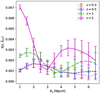 |
Fig. A.1. Function S defined in Eq. (10), evaluated at the constant volume threshold, λCV, for different redshifts and co-moving smoothing lengths, Rs. The error bars indicate the σ region of the cosmic variance. |
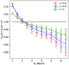 |
Fig. A.2. Ratio between λCV calculated for a snapshot with redshift, z, and the λCV value calculated for a snapshot with redshift z = 2. The black line shows the value 1. |
Appendix B: CW density
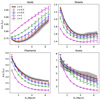 |
Fig. B.1. Total density of each CW element, defined as mass fraction divided by volume fraction computed using |

In the same way that we have used the volume fraction as a measure of the statistical presence, the mass fraction gives us clues about the evolution of the dark matter distribution in CW. More specifically, measuring the time dependence gives us information on the mass transfer between the different elements, as well as which of them are more populated with matter than others. We can define the mass fraction of a CW element as the total mass that is classified as that element divided by the total mass inside the simulated box. If we divide the mass fraction fm by the volume fraction fv, we get an estimate of the total density Δ occupied by a certain element:
 (B.1)
(B.1)
Figure B.1 shows the density of each of the CW components at constant volume threshold. When applying the methodology of Sect. 3 to mass fractions instead of volume fractions there is no conservation at any threshold. This causes the density to have a clear evolution as can be seen in Fig. B.1, including the extrapolation to z = 0. As Δ decreases with time for voids in all Rs values, the opposite occurs for sheets and filaments. Similar behaviour has also been observed in other works on mass evolution in the CW (e.g. Cautun et al. 2014; Zhu & Feng 2017).
Appendix C: Reference redshift
We have used z = 0 as the reference for the re-scaling (8), but our results and conclusions will also hold for any other reference redshift. A simple proof of this is given in this appendix.
Suppose we use as a reference z = 0. We denote the use of this reference by “|z = 0”. Let be a certain threshold value at the reference redshift λth|z = 0. We can calculate the equivalent of this threshold at another redshift z by the re-scaling (8), which we will denote as  . Therefore, while z = 0 is the reference (as has been done throughout the paper), clearly
 (C.1)
(C.1)
If in this reference we want to find the threshold λth|z = 0 from a threshold at a specific redshift, zr:
 (C.2)
(C.2)
Suppose now that we change the reference redshift to zr. To find its equivalent at z = 0, we use the re-scaling
 (C.3)
(C.3)
Since we are dealing with the same two numbers, we can compare Eqs. (C.2) and (C.3):
 (C.4)
(C.4)
To find  in the reference of zr we use
 (C.5)
(C.5)
 (C.6)
(C.6)
finally proving that
 (C.7)
(C.7)
which means that the classification obtained by applying  to the V-web in snapshot z remains unchanged for different reference redshifts.
All Tables
All Figures
|
Fig. 1. Density and V-web classification of a gravity-only ΛCDM simulation. The cube is divided into a Ng = 5123 cells grid on which both the density and the eigenvalues of the shear velocity tensor have been calculated, applying a smoothing of Rs = 1 Mpc/h. Panels a and b show the logarithm of the DM density at redshifts 2 and 0 respectively (in a slice that has a thickness of ∼1.5 Mpc/h). Panels c and d contain, for the previous redshifts, the classification into CW elements performed by the V-web method for an λth = 0 (in a middle slice that is one grid cell thick). Panels e and f contain the same as the previous two, but for the λth = 0.44 proposed by Hoffman et al. (2012). |
| In the text | |
|
Fig. 2. Volume fractions of the CW elements obtained with V-web from a simulation shown in Fig. 1. The left panel show the results using the same threshold for all redshifts, while in the right panels, Eq. (8) has been used to normalize λth. The applied smoothing length is Rs = 3 Mpc/h. |
| In the text | |
|
Fig. 3. Evolution of the difference in volume fractions after λth normalization defined in Eq. (8). Each line is the volume fraction at z = 0 minus the volume fraction at other redshifts (differentiated with the type of pattern), as a function of λth. The colour code, simulation, and RS value is the same as the one used in Fig. 2. The magenta circle marks the constant volume threshold λCV in which the volume fractions of each element become approximately constant over time. |
| In the text | |
|
Fig. 4. Function S defined in Eq. (10) calculated for the simulation of the previous figures (Rs = 3 Mpc/h). The magenta circle marks S(λCV). |
| In the text | |
|
Fig. 5. Mean of λCV computed using the minimum of the function S in each simulation of our set, shown as solid lines. The dashed lines correspond to the fit defined in Eq. (13), as explained in Sect. 5.1. The different colours correspond to the smoothing length used in the analysis, with the shading indicating the σ region of the set. |
| In the text | |
|
Fig. 6. Mean of λCV for different redshifts, as a function of the smoothing length, Rs. The error bars indicate the σ region of the set. |
| In the text | |
|
Fig. 7. V-web classification of the simulation shown in Fig. 1, applying in this case the threshold |
| In the text | |
|
Fig. 8. Mean volume fractions for different CW elements computed using |
| In the text | |
|
Fig. 9. Parameters a and b defined in Eq. (12) and measured by least squares applied to each value of Rs used to obtain λCV in the MG-COLA set of simulations. The error bars (small in the right panel) are given by the square root of the diagonal elements in the covariance matrix. Both parameters have been approximated to an exponential type function plotted in red, whose constants are given in Table 4. The result of the approximation is a fit |
| In the text | |
|
Fig. 10. Differences in volume fractions at different redshifts (shown in the first three panels) calculated for an off-set Gadget simulation. The constant volume threshold phenomenon appears for all classified elements despite the fact that the cosmology, box size, initial conditions, and code are different from those of the MG-COLA set used in the rest of the work. The black vertical area shows the calculated range for |
| In the text | |
|
Fig. A.1. Function S defined in Eq. (10), evaluated at the constant volume threshold, λCV, for different redshifts and co-moving smoothing lengths, Rs. The error bars indicate the σ region of the cosmic variance. |
| In the text | |
|
Fig. A.2. Ratio between λCV calculated for a snapshot with redshift, z, and the λCV value calculated for a snapshot with redshift z = 2. The black line shows the value 1. |
| In the text | |
|
Fig. B.1. Total density of each CW element, defined as mass fraction divided by volume fraction computed using |
| In the text | |
Current usage metrics show cumulative count of Article Views (full-text article views including HTML views, PDF and ePub downloads, according to the available data) and Abstracts Views on Vision4Press platform.
Data correspond to usage on the plateform after 2015. The current usage metrics is available 48-96 hours after online publication and is updated daily on week days.
Initial download of the metrics may take a while.