| Issue |
A&A
Volume 661, May 2022
|
|
|---|---|---|
| Article Number | A146 | |
| Number of page(s) | 14 | |
| Section | Cosmology (including clusters of galaxies) | |
| DOI | https://doi.org/10.1051/0004-6361/202142852 | |
| Published online | 24 May 2022 | |
Cosmology with cosmic web environments
I. Real-space power spectra
1
Université Paris-Saclay, CNRS, Institut d’Astrophysique Spatiale, 91405 Orsay, France
e-mail: This email address is being protected from spambots. You need JavaScript enabled to view it.
2
Université Paris-Saclay, TAU team INRIA Saclay, CNRS, Laboratoire Interdisciplinaire des Sciences du Numérique, 91190 Gif-sur-Yvette, France
3
Laboratoire de Physique de l’École normale supérieure, ENS, Université PSL, CNRS, Sorbonne Université, Université de Paris, 75005 Paris, France
4
Departamento de Física Téorica I, Universidad Complutense, 28040 Madrid, Spain
Received:
7
December
2021
Accepted:
19
February
2022
Abstract
We undertake the first comprehensive and quantitative real-space analysis of the cosmological information content in the environments of the cosmic web (voids, filaments, walls, and nodes) up to non-linear scales, k = 0.5 h Mpc−1. Relying on the large set of N-body simulations from the Quijote suite, the environments are defined through the eigenvalues of the tidal tensor and the Fisher formalism is used to assess the constraining power of the spectra derived in each of the four environments and their combination. Our results show that there is more information available in the environment-dependent power spectra – both individually and when combined – than in the matter power spectrum. By breaking some key degeneracies between parameters of the cosmological model such as Mν–σ8 or Ωm–σ8, the power spectra computed in identified environments improve the constraints on cosmological parameters by factors of ∼15 for the summed neutrino mass Mν and ∼8 for the matter density Ωm over those derived from the matter power spectrum. We show that these tighter constraints are obtained for a wide range of the maximum scale, from kmax = 0.1 h Mpc−1 to highly non-linear regimes with kmax = 0.5 h Mpc−1. We also report an eight times higher value of the signal-to-noise ratio for the combination of environment-dependent power spectra than for the matter spectrum. Importantly, we show that all the results presented here are robust to variations of the parameters defining the environments, suggesting a robustness to the definition we chose to extract them.
Key words: cosmology: theory / large-scale structure of Universe / cosmological parameters
© T. Bonnaire et al. 2022
 Open Access article, published by EDP Sciences, under the terms of the Creative Commons Attribution License (https://creativecommons.org/licenses/by/4.0), which permits unrestricted use, distribution, and reproduction in any medium, provided the original work is properly cited.
1. Introduction
One of the successes of modern cosmology is the observation of the matter distribution at megaparsec scales, for which both data and simulations are available. This impressive pattern, commonly referred to as the cosmic web (Klypin & Shandarin 1983; Bond et al. 1996), was first observed in galaxy surveys like the Center for Astrophysics Redshift Survey (de Lapparent et al. 1987) and was recently traced more precisely by other redshift surveys like the Sloan Digital Sky Survey (SDSS, York et al. 2000) or the Two-Micro All Sky Survey (2MASS, Skrutskie et al. 2006). In this multi-scale pattern, isolated clumps of matter residing in empty under-dense parts of the Universe are flowing into flattened planar-like regions and are then funnelled into tubular elongated structures to finally end their journey by feeding large and massive anchors. The formation of these cosmic structures, called voids, walls, filaments, and nodes, respectively, was predicted by pioneering analytical models in the seventies (Zel’dovich 1970; Doroshkevich & Shandarin 1978), which linked the gravitational collapse of the primordial density fluctuations, assumed and observed to be Gaussian distributed, to the formation of anisotropic structures. This non-linear gravitational evolution yields a non-Gaussian distribution of the matter at late time with strong mode couplings in which the information is spread over higher order correlations. It is well established that the way matter evolves and clusters through time and under the effect of gravity is highly impacted by the initial density perturbations and by the underlying cosmological model described by the values of the cosmological parameters.
Despite the non-Gaussian nature of the matter distribution at low redshifts, basic summary statistics like the one-point probability distribution function and the two-point correlation function, or the Fourier-equivalent power spectrum, constitute a wealthy source of information about the cosmological model that can be used in practice through the sparse and biased observation of tracers such as galaxies to constrain cosmological parameters (e.g., Cole et al. 2005; Tinker et al. 2012; Alam et al. 2017; Gruen et al. 2016, 2018; Gil-Marín et al. 2017; Uhlemann et al. 2020).
Numerous works also show that the first higher order term, namely the bispectrum, carries non-negligible information able to improve the constraints (Sefusatti et al. 2006; Yankelevich & Porciani 2019; Hahn et al. 2020; Hahn & Villaescusa-Navarro 2021; Agarwal et al. 2021; Gualdi et al. 2021). However, because of the difficulties of directly measuring and computing higher order statistics (see e.g., Schmittfull et al. 2013; Philcox 2021), alternative methods were proposed to account only partially, or indirectly, for higher order terms. Example of these methods are the minimum spanning tree analysis from Naidoo et al. (2020, 2022) and ‘marked statistics’ (Stoyan 1984). The latter enables the computation of a weighed version of the two-point information in which a mark is assigned to each tracer, for example a galaxy, halo, or particle, based for instance on the local luminosity (Beisbart & Kerscher 2000; Sheth et al. 2005) or density (White 2016). More recently, the wavelet scattering transform (Mallat 2012) also introduced a non-linear transformation of the input density field to extract further information by cascading convolutions with directional wavelet filters and was successfully applied to cosmological simulations (see e.g., Allys et al. 2019, 2020; Cheng et al. 2020; Cheng & Ménard 2021). These last two approaches were shown to improve the constraints over the real-space matter power spectrum by Massara et al. (2021) and Valogiannis & Dvorkin (2021), respectively. Other works make use of direct additional observables to the density field, such as the velocity, to improve the constraints on cosmological models and parameters (e.g., Mueller et al. 2015; Kuruvilla & Aghanim 2021; Kuruvilla 2022).
While substantial efforts are being made to link the properties of cosmic web elements (mainly clusters and filaments) to the formation and evolution of matter tracers like galaxies (see e.g., Alpaslan et al. 2014; Malavasi et al. 2017, 2022; Codis et al. 2018; Bonjean et al. 2018, 2020), little is currently known about the information these environments carry about the underlying cosmological model. Strong focus has been placed on the use of the densest and therefore most easily identified elements of the cosmic web, namely nodes. The hierarchical structure formation makes them particularly interesting for probing not only the matter and dark energy contents of the Universe (e.g., Bahcall et al. 1997; Bahcall & Fan 1998; Holder et al. 2001; Salvati et al. 2018; Marulli et al. 2018) but also the amplitude of the initial density fluctuations (for a review, see Allen et al. 2011). The clustering properties of the other extreme environment represented by voids also drew the attention of cosmologists, who used these to probe the accelerated expansion of the Universe and the summed neutrino mass (Lee & Park 2009; Lavaux & Wandelt 2012; Pisani et al. 2015). The extent of void clustering as well as their size, shape, number, bias, and corresponding evolution with redshift are therefore key quantities probing the underlying cosmological model (van de Weygaert & Platen 2011; Hamaus et al. 2014, 2015; Massara et al. 2015; Schuster et al. 2019; Kreisch et al. 2019). The constraints brought by these two extreme environments, that is voids and nodes, are for example combined in Bayer et al. (2021) and Kreisch et al. (2021), who show that the information provided by the halo mass function and the void size function leads to considerable improvement of the matter power spectrum constraints in real space.
However, cosmic web complexity and its full pattern go beyond the picture provided by the properties of voids and nodes. We can expect that, when splitting the matter into the various environments, a simple two-point statistical analysis would deliver different information, which when combined may break degeneracies and improve the constraints on cosmological parameters. These expectations are in line with the recent findings of Paillas et al. (2021) in which the two-point correlation function computed from galaxies in several density bins improves the cosmological constraints in redshift space. In the present paper, we present a first thorough analysis of the cosmological information of the matter distribution in the several cosmic web environments identified by means of the eigenvalues of the tidal tensor and through the power spectrum statistic in the derived density fields. From the intrinsic differences in densities, tidal force, and anisotropies exhibited by these environments, we explore their distinct sensitivities to the variations of cosmological parameters. After introducing the N-body simulations used in our analysis in Sect. 2, we present our methodological approach in Sect. 3, presenting and assessing the environments definition and defining the power spectrum estimator. In Sect. 4, we then present the Fisher formalism and report the constraints obtained on the six studied cosmological parameters using the power spectrum derived from each environment individually and from their combination. In Sect. 5, we discuss the obtained results and compare them with other recent findings. After drawing some conclusions from this work and offering future and perspectives in Sect. 6, we present a study of the convergence and assumptions of the analysis in the Appendices.
2. The Quijote simulations
Quijote (Villaescusa-Navarro et al. 2020) is a publicly available1 large suite of N-body simulations. With 44 100 simulations spanning more than a thousand cosmological models, each with multiple realisations, it is an ideal dataset with which to perform statistical cosmological analyses as it allows us to build accurate covariance matrices and compute derivatives for any cosmological representation. Each simulation consists of a set of 5123 particles (and 5123 neutrinos in massive neutrinos cases) that are evolved forward in time from z = 127 to z = 0 using a tree-PM Gadget-3 code (Springel 2005) in a box of L = 1 Gpc h−1 in size initialised with the second-order Lagrangian perturbation theory for massless neutrino simulations and with the Zel’dovich approximation for massive neutrino simulations. The fiducial cosmology is a flat ΛCDM cosmology with parameters consistent with Planck Collaboration VI (2020): Ωm = 0.3175, Ωb = 0.049, h = 0.6711, ns = 0.9624, and σ8 = 0.834. With these parameters, and assuming zero mass for neutrinos (Mν = 0), 15 000 random realisations are computed. The Quijote suite then provides 500 realisations by varying each parameter individually, fixing the others at their fiducial values. The step sizes are: dΩm = 0.010, dΩb = 0.002, dh = 0.020, dns = 0.020, and dσ8 = 0.015. Additionally, 500 realisations using several sums of neutrino mass are also computed, with Mν = ∑mν = {0.1, 0.2, 0.4} eV, which we refer to as  ,
,  and
and  cosmologies, respectively. Because massive neutrino simulations are initialised with the Zel’dovich approximation, we also use, for consistency, a massless neutrino simulation initialised this way for the computation of derivatives with respect to Mν.
3. Cosmic web environments: segmentation and statistics
3.1. Cosmic web segmentation
Over the past decades, several methods have been proposed to identify cosmic structures in either simulations or observations. Some algorithms directly rely on the density field as an input and base their definition on the curvature of the density or the gravitational field (such as Hahn et al. 2007; Forero-Romero et al. 2009; Aragon-Calvo et al. 2010a; Cautun et al. 2013) or on its topological description (Aragón-Calvo et al. 2010b; Sousbie 2011). Other algorithms rely on more observable inputs, such as the sparse distribution of galaxies (or halos in simulations), to identify structures such as filaments through geometrical principles (Stoica et al. 2007; Chen et al. 2015; Tempel et al. 2016) or based on graph theory (such as Barrow et al. 1985; Alpaslan et al. 2014; Bonnaire et al. 2020, 2021; Pereyra et al. 2020). In the present theoretical work, we aim to study all the cosmic web environments (voids, walls, filaments, and nodes) based on the dark matter particles of the Quijote simulations. To achieve that, we choose a web finder that defines environments in a physical way based on the local level of tidal anisotropy using prescriptions originating from the linear growth of perturbations in the Zel’dovich approximation (Zel’dovich 1970). Following the formalism introduced in Hahn et al. (2007), and later extended by Forero-Romero et al. (2009), we identify the environments in the simulations through the tidal tensor T, hereafter referred to as T-web formalism. From the discrete set of particle positions, we first rely on a B-spline interpolation scheme (Hockney & Eastwood 1981; Sefusatti et al. 2016) to estimate the density field ρ(x) on an  regular grid. For our purposes, we adopt an interpolation of order four, namely the piecewise-cubic spline (PCS) scheme, in which the mass of a particle is spread over the 43 = 64 closest cells. By noting d = Ng∥x − xp∥2/L with x being the centre of a grid cell, xp the particle position, and L the size of the box length (assuming a cubic box), PCS weights are given by
 (1)
(1)
This choice of interpolation order is a good trade-off between the accuracy of the reconstructed field and its computational time.
From the density field ρ, we derive the gravitational potential Φ by solving the Poisson equation
 (2)
(2)
where Δ is the Laplacian operator and G is the gravitational constant. It is convenient to write this equation in terms of the reduced gravitational potential  , with
  being the averaged density, so that Eq. (2) satisfies ΔΦr(x)=δ(x), with
  the overdensity. Solving this reduced version of the Poisson equation in Fourier space using a discrete approximation of the Laplacian operator (in our case, a seven-point approximation) holds an estimate of Φ(x) on the grid. From the gravitational potential, we obtain the tidal tensor in each grid cell x as
 (3)
(3)
leading to the field of eigenvalues λ1(x) ≤ λ2(x) ≤ λ3(x). The cosmic environment associated with a grid cell x is finally obtained depending on the number of eigenvalues below a given threshold λth, as defined in Table 1.
Cosmic web classification rules in the cell x depending on the eigenvalues λ1 ≤ λ2 ≤ λ3 of the tidal tensor.
We then use the segmentation of the density field obtained at the cell level to build individual overdensity fields for each environment. To do so, we simply propagate the classes at the particle level by assigning the same environment signature to all hosted particles in a given cell. Even though more sophisticated schemes have been proposed (see e.g., Wang et al. 2020), we expect this approach to be sufficiently robust for the particles at hand, but other methods could be of use when applying the procedure to coarser structures like halos. Based on the PCS interpolation scheme, we then build four corresponding overdensity fields {δv, δw, δf, δn} where the subscripts respectively refer to void, wall, filament, and node environment. The matter density field δm is therefore decomposed into the four environmental fields and fulfils the linear combination
 (4)
(4)
where fα denotes the mass fraction of the environment α, where Nα/N is the number of particles in the α environment and N the total number of particles2. In Fig. 1 we show this decomposition with the contribution of each environment to the overall matter density field for a thin 2.77 Mpc h−1 depth slice. As expected, nodes describe a discrete set of dense objects found at the intersections of filaments and voids cover most of the surface with large low-density areas.
 |
Fig. 1. Overdensity fields computed in the different environments. From top to bottom: set of five 2.77 Mpc h−1 depth slices showing the fields δm, δv, δf, δw, and δn, respectively. Overdensity fields in cosmic web environments are computed from the T-web classification of particles and are normalised such that δm = ∑αfαδα. |
3.2. Choice of the parameters
In our implementation of the T-web formalism, the potential is smoothed with a Gaussian of standard deviation σ𝒩 Mpc h−1 before the classification. The full segmentation procedure therefore depends on three parameters, which are: σ𝒩, the Gaussian smoothing scale, Ng, the total number of grid cells, and λth, the threshold for the eigenvalues of the tidal tensor. Both Ng and σ𝒩 are related to a smoothing effect of the fields and can be combined in an effective smoothing scale defined as  . The choice of Ng represents a trade-off between the minimum scales involved in the analysis and the resolution of the simulation containing, in the present case, 5123 particles. To be able to probe non-linear scales up to around 0.5 h Mpc−1, we find that Ng = 360 is a good choice, leading to a half-Nyquist frequency of kNyq/2 = 0.57 h Mpc−1, with kNyq = πNg/L. In practice, we set kmax = 0.5 h Mpc−1, allowing us to take into account both large and non-linear scales without introducing bias induced by aliasing effects occurring when k > kNyq/2. On the other hand, σ𝒩 blurs out structures at scales below this value. Physically, the sizes of the structures (radii of nodes, widths of filaments and walls) spread over a few Mpc h−1 (Cautun et al. 2014). If we want to accurately describe the structures whilst still aiming at a target scale of 12.5 Mpc h−1 in configuration space (corresponding to a Fourier mode of 0.5 h Mpc−1), Reff should be limited so that some voxels can be used to probe it. Consequently, for Reff to be below 4 Mpc h−1 and with Ng = 360, σ𝒩 should be below 3 Mpc h−1. In practice, we adopt σ𝒩 = 2 Mpc h−1, leading to an effective smoothing scale of Reff = 3.4 Mpc h−1. After assessing several reasonable values of σ𝒩 ∈ [1.5,2.5] Mpc h−1, we find that the volume fractions are changed by less than a percent while the mass fractions are modified by around 3%. The chosen fiducial value of the smoothing scale is also coherent with previous usage of Gaussian smoothing for continuous fields before applying Hessian-based classification methods (e.g., Hahn et al. 2007; Cautun et al. 2013, 2014; Martizzi et al. 2019).
However, the λth parameter has a greater effect on the classification of environments, both in terms of volume and mass fraction (Forero-Romero et al. 2009). The impact of this parameter is illustrated in Fig. 2, which shows the averaged mass fractions ⟨fα⟩ for each cosmic web environment as drawn by the T-web formalism with three values of  . The fiducial value of 0.3 corresponds roughly to the threshold at which voids percolate for the cosmological volume of L3 = 1 (Gpc/h)3 (Forero-Romero et al. 2009). Figure 2 reports the mass fractions obtained with these three values of λth, showing that an increasing number of particles is associated with voids and less with filaments and nodes when the threshold is increased. More quantitatively, varying λth from 0.2 to 0.4 leads to a factor of two difference between the obtained mass fractions in voids.
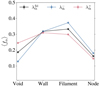 |
Fig. 2. Averaged mass fractions ⟨fα⟩ in the different cosmic web environments for distinct values of |
In order to derive constraints from environments that are robust to the identification of the environments and therefore indirectly robust to changes in the definitions of the various web-finder methods (see e.g., Libeskind et al. 2017), we embed both σ𝒩 and λth as nuisance parameters in the analysis such that all presented cosmological constraints are marginalised over them.
3.3. Cosmological sensitivity of the classification
Figure 3 shows the ratio between the averaged mass fractions in each environment when a cosmological parameter varies and the average obtained with the fiducial cosmology,  . The error bars (represented by the bars around points and crosses, and by the grey shaded area for fiducial simulations) are the 3σ confidence intervals. Many cosmological parameters cause sizeable changes in these proportions, and parameters related to matter density, like σ8 and Ωm, are among those having the greatest impact, together with ns. The most notable variations are induced by σ8, where an increase (respectively decrease) leads to a larger (respectively smaller) mass fraction in dense environments (nodes and filaments). This is in agreement with the definition of σ8 that is measuring how matter clusters at a scale of 8 Mpc h−1. The impact of neutrino mass, even though smaller in comparison, is significant with fraction ratios lying outside the 3σ confidence regions when varying this parameter. The right panel of Fig. 3 shows that, similarly to the effect of σ8, increasing Mν makes dense environments even denser. All these different effects observed in the mass fractions already suggest that each cosmological parameter has a different impact on the environments; these effects can be further refined when inspecting the information contained in the power spectra.
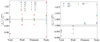 |
Fig. 3. Ratios between mass fractions in the cosmic web environments and mass fractions obtained with fiducial cosmology for an eigenvalue threshold of |

3.4. Power spectra in cosmic web environments
The auto power spectrum Pαα(k) is defined as the covariance of Fourier modes of the overdensity field δα, with α ∈ {v, w, f, n} denoting voids, walls, filaments, and nodes, respectively. For an overdensity field δα, the power spectrum is given by
 (5)
(5)
with k = ∥k1∥2,  referring to the Fourier transform of δ, and
  is the Dirac delta distribution in ℝ3. For simulations with Mν > 0, power spectra are computed based on the total matter density fields containing both dark matter and neutrino particles, δm = fCDMδCDM + fνδν, where δν is the neutrino field and δCDM is the field of dark matter particles. The fraction fν is computed as Ων/Ωm with Ων = Mνh−2/93.14 eV and fν + fCDM = 1.
However, the PCS smoothing scheme used to evaluate the overdensity fields δα deforms the shape of the estimated power spectra (Jing 2005), and we correct for this effect by first deconvolving the fields δα through the application of the window function in Fourier space
![Mathematical equation: $$ \begin{aligned} W(k) = \left[ \prod _i \left(1 - \frac{4}{3} s_i + \frac{2}{5} s_i^2 - \frac{4}{315} s_i^3 \right) \right]^{-1}, \end{aligned} $$](/articles/aa/full_html/2022/05/aa42852-21/aa42852-21-eq20.gif) (6)
(6)
with si = sin(πki/2kNyq) and kNyq the Nyquist frequency. Finally, because of the discrete nature of the input, namely the dark matter particles (or the neutrinos in massive neutrino simulations), we also subtract the shot noise contribution from power spectra estimated with Eq. (5). Even though the number of particles is very large and we expect the shot noise contribution to be small at the scales of interest, auto-spectra Pαα (including also Pmm) are subtracted by the quantity 1/n̄α where n̄α = Nα/L3. In massive neutrino simulations, the shot noise is removed from the two weighed discrete contributions of the dark matter and the neutrino particles. However, this latter is expected to be small on the overall power spectra because of the  weight which is small in the explored values of Mν.
The auto-spectra are computed with a spectral bin size dk = 2kf with kf = 2πNg/L ≃ 0.0126 h Mpc−1. For a maximum scale of kmax = 0.5 h Mpc−1, this yields 40 bins in Fourier space for each environment, as well as for the matter spectra. The various auto-spectra Pαα(k) are shown in Fig. 4 in their normalised versions  in order to better visualise the contributions of each environment to the overall matter spectrum Pmm(k). We qualitatively observe different shapes with Pff(k), which globally resembles a shift of the matter power spectrum, which is emphasised in the bottom panel where the ratios to Pmm(k) are shown. However, node, void, and wall auto-spectra show different shape dependencies. In particular, we note that, at large scales (k < 0.13 h Mpc−1), the dominant contribution is associated with filaments while most of the power is contained in nodes at smaller scales. Also, at large scales, Pvv(k) and Pww(k) share similar amplitudes but the former quickly decreases when k > 0.05 h Mpc−1 with respect to all other environments. These different k-dependencies reflect the dissimilar statistical distributions of the matter in several cosmic web environments.
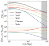 |
Fig. 4. Top panel: real-space normalised power spectra |

4. Cosmological information content of cosmic web environments
4.1. Fisher formalism
Considering a set of model parameters θ ∈ ℝd (cosmological parameters in our case), we assume that the vector s ∈ ℝn is a statistic built from an observable (here, the binned power spectra drawn from the overdensity fields) following a Gaussian distribution  . Its log-likelihood can therefore be written
 (7)
(7)
where the constant comes from the normalisation of the distribution. A common way to quantify the information carried by s on θ is to use the Fisher information matrix I(θ). From the Fréchet-Darmois-Cramér-Rao inequality, its inverse I(θ)−1 corresponds to a lower bound on the variance of any unbiased estimator drawn from s, which can therefore be used to assess the efficiency of the representation. Elements of the Fisher matrix are defined as the variance of the derivative of the log-likelihood, namely
![Mathematical equation: $$ \begin{aligned} \left[ \boldsymbol{I}(\boldsymbol{\theta }) \right]_{i,j} = \mathbb{E} _\theta \left[ \left(\frac{\partial \log p(\boldsymbol{s} \,|\,\boldsymbol{\theta })}{\partial \theta _i}\right)^\mathsf{T }\left( \frac{\partial \log p(\boldsymbol{s} \,|\,\boldsymbol{\theta })}{\partial \theta _j} \right) \right], \end{aligned} $$](/articles/aa/full_html/2022/05/aa42852-21/aa42852-21-eq26.gif) (8)
(8)
which can also be written in terms of the second derivative of the log-likelihood under some smoothness constraints (which are fulfilled in the Gaussian case),
![Mathematical equation: $$ \begin{aligned} \left[ \boldsymbol{I}(\boldsymbol{\theta }) \right]_{i,j} = -\mathbb{E} _\theta \left[ \frac{\partial ^2 \log p(\boldsymbol{s} \,|\,\boldsymbol{\theta })}{\partial \theta _i\partial \theta _j} \right], \end{aligned} $$](/articles/aa/full_html/2022/05/aa42852-21/aa42852-21-eq27.gif) (9)
(9)
where 𝔼θ is the expectation taken over the distribution p(s | θ). This latter equation intuitively explains how the amount of information is measured. A sharp log-likelihood around θ implies a huge increase with small changes of the parameters, making the statistic s very sensitive to variations dθ. On the other hand, a weakly curved log-likelihood with a locally flat behaviour advocates for a poor representative power of the statistic because its sensitivity to changes of the parameters is low. Under the Gaussian assumption described above and by further considering a covariance matrix Σ independent of cosmological parameters θ, mainly because this contribution is expected to be small and a source of underestimation of errors (Carron 2013; Kodwani et al. 2019), the Fisher information matrix reads
![Mathematical equation: $$ \begin{aligned} \left[ \boldsymbol{I}(\boldsymbol{\theta }) \right]_{i,j} = \left(\frac{\partial \bar{\boldsymbol{s}}}{\partial \theta _i}\right)^\mathsf{T }\boldsymbol{\Sigma }^{-1} \left(\frac{\partial \bar{\boldsymbol{s}}}{\partial \theta _j}\right). \end{aligned} $$](/articles/aa/full_html/2022/05/aa42852-21/aa42852-21-eq28.gif) (10)
(10)
The non-linear operation of the inversion to compute the precision matrix Σ−1 leads to a biased estimate, although the covariance can be computed using the classical unbiased estimation. Under the previously established Gaussian assumption, the unbiased estimate of the precision matrix is given by (Kaufman 1967; Hartlap et al. 2007)
 (11)
(11)
where Nfid is the number simulation at the fiducial cosmology, n is the length of the summary statistics vector s, and  is the unbiased estimate of the covariance matrix.
In our study, the partial derivatives of the summary statistics with respect to parameters of the model can be computed numerically using the variations of cosmologies provided by the Quijote suite of simulations. Considering the set of cosmological parameters studied here, {Ωm, Ωb, h, ns, σ8}, we can estimate
 (12)
(12)
In the case of massive neutrino simulations, Mν > 0 with a fiducial value at 0.0 eV. For this parameter, we therefore cannot rely on Eq. (12) and instead estimate the derivative using the four-point forward approximation
 (13)
(13)
Because massive neutrino simulations in Quijote are initialised using the Zel’dovich approximation and fiducial simulations are initialised using the second-order Lagrangian perturbation theory, the quantity  is computed using the fiducial simulations initialised along with the Zel’dovich approximation. In all the presented results, unless stated otherwise, the numerical estimation of derivatives and covariances has been made with Nderiv = 500 and Nfid = 7000 realisations, respectively. In Appendix A, we discuss the impact of these numbers and assess the numerical stability of the results.
4.2. Information content of power spectra in cosmic web environments
The two key ingredients of the Fisher-based quantification of information appear in Eq. (10) as the covariance matrix Σ and the partial derivatives of the statistic with respect to the cosmological parameters. Figure 5 plots a proxy of the first ingredient through the normalised version of the covariance matrix, namely the correlation matrix C, whose elements are defined as
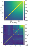 |
Fig. 5. Correlation coefficients Cij for the matter power spectrum (top) and the power spectra in the several environments (bottom). Each submatrix goes from k = 0.1 h Mpc−1 to k = 0.5 h Mpc−1. |
 (14)
(14)
The first striking observation when inspecting the correlation matrix for Pmm in the top panel of Fig. 5 is that it quickly becomes highly non-diagonal with correlation coefficients Ck1, k2 = 0.5 at scales of ∼0.3 h Mpc−1. Such high couplings between scales are expected at low redshifts, with Fourier modes being increasingly correlated with time, as a result of the non-linear evolution of the matter distribution (see Blot et al. 2015). These non-diagonal terms intrinsically reduce the representative power of the matter power spectrum to constrain the cosmological parameters, independently of how it varies with these latter. The power spectra in different environments – shown in the bottom panel of Fig. 5 – display less off-diagonal cross-correlation coefficients of high values, except in the node-node case. Indeed, Fourier modes of Pnn are highly correlated with values Ck1k2 ∼ 0.5 for k1, k2 ∼ 0.2 h Mpc−1, which is a signature of the highly non-linear environment it represents. Other environments display lower values of the correlation coefficients at similar scales, with ∼10−1 for filaments, ∼10−2 for walls, and ∼5 × 10⁻² for voids. Fewer and fewer correlations between modes are therefore observed in environments with decreasing |δ|, from non-linear regions like nodes and filaments, followed by mildly non-linear voids, and finally walls having the distribution of densities closest to zero, being consequently the environment exhibiting the least coupling between Fourier modes, as can be visually appreciated from Fig. 5.
Figure 6 shows the second ingredient of the Fisher-forecast formalism: the partial derivatives for all the studied statistics. Compared to Pmm, the spectra drawn from the cosmic web environments show different patterns in the derivatives, probing broader ranges of amplitudes and exhibiting different features. Taking the example of the Ωm parameter in the top left panel, the change of sign occurs at different scales for each environment, and seems to follow the order of average density, namely from voids to nodes. This pattern is also observed for other parameters like Ωb, h, ns, and Mν. The similar k-dependencies observed between the partial derivatives of the matter power spectrum demonstrates the limitation of this statistic in discriminating between the effects of different cosmological parameters. Showing various dependencies, the power spectra in the cosmic web environments appear to provide different information on the set of cosmological parameters, and when combined all together, they may break degeneracies and allow us to put tighter constraints on the underlying cosmological model.
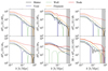 |
Fig. 6. Partial derivatives ∂Pαα(k)/∂θi for the different environmental auto-spectra and for each studied parameter {Ωm, Ωb, h, ns, σ8, Mν}. Dashed (respectively solid) lines correspond to negative (respectively positive) values of the derivative. The grey area depicts the range of k > kmax excluded from the analysis. |
One way to quantify the information gained from the power spectra in the environments is to compute the marginalised 1σ confidence ellipses that can be obtained from the Fisher information matrices (10). These latter are shown in Fig. 7 when using the matter power spectrum or those from each environment either individually or combined. Table 2 gathers the marginalised σθi constraints obtained in the different cases defined as
![Mathematical equation: $$ \begin{aligned} \sigma _{\theta _i} = \frac{1}{\sqrt{\left[\boldsymbol{I}(\boldsymbol{\theta })^{-1}\right]_{i,i}}}, \end{aligned} $$](/articles/aa/full_html/2022/05/aa42852-21/aa42852-21-eq35.gif) (15)
(15)
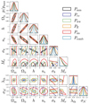 |
Fig. 7. 1σ confidence ellipses for all the pairs of cosmological (Ωm,Ωb,h,ns,σ8,Mν) and nuisance (λth) parameters obtained from the matter power spectrum, or the spectra from the different environments and their combination in real space. The normalised probability density function for each parameter is shown on the diagonal. |
Marginalised 1-σ constraints obtained from the power spectrum in different environments for all cosmological parameters in real space and considering λth and σ𝒩 as nuisance parameters.
where Ii, i is the ith diagonal element of the Fisher information matrix. The corner plot of Fig. 7 exhibits the degeneracies among parameters in almost all panels with black elongated ellipses translating the limitation of Pmm in distinguishing between the effect of varying one or other parameter, which is already suggested by the shapes of the derivatives. This is for instance observed in the Mν–σ8 panel (also reported and studied in previous works such as Villaescusa-Navarro et al. 2013, 2014; Peloso et al. 2015), or the panel showing Ωm–σ8. When inspecting the ellipses obtained from the spectra computed in the individual environments, we clearly distinguish different orientations for several parameters. It is for instance especially striking in the Mν–σ8 plane where Pff and Pvv are showing quasi-orthogonal ellipses, but also in the projected space involving σ8 and h, ns, or Ωb. This illustrates the complementary information delivered by the two-point statistic in cosmic web environments, which, when combined all together, tightens up the constraints as quantitatively shown in Table 2 with improvement factors over the matter power spectrum ranging from 2.9 to 15.7 for the five cosmological parameters considered and 15.2 for the sum of neutrino mass. The different structures observed in the derivatives of Fig. 6 and the individually lower couplings between k modes in the covariance matrices from the bottom panel of Fig. 5 also translate into better constraints for some environments and parameters, except nodes and σ8. The high level of correlation brought by the Pnn coefficients and the small range of amplitudes probed by their derivatives indeed lead to large errors on cosmological parameters when exploiting this environment alone. Without similar high couplings, the other environments perform either equivalently or better than the matter power spectrum in most cases. It is worth noting that these constraints do not take into account any additional prior information coming from other measurements that could improve them even further, such as information from the cosmic microwave background (CMB) experiments (Planck Collaboration VI 2020).
The results presented above were obtained by including λth and σ𝒩 as nuisance parameters. When fixing those to their fiducial values, we obtain the constraints reported in Table C.1, which are quasi-identical for Pcomb on cosmological parameters Ωm, Ωb, h, and ns. Adding the nuisance parameters and marginalising over them mainly impacts σ8 and Mν where the improvement factors are respectively lowered down from 7.2 and 24.3 to 2.9 and 15.2. This is mainly due to the additional degeneracies induced by the two additional parameters, with for instance σ8 and σ𝒩 which have similar effects on the power spectra, mainly a shift (also visible from the corresponding panel in Fig. 7). The obtained results from Pcomb therefore show good robustness to these nuisance parameters, given their impact on the segmentation of the environments and on the derived statistics. Quantitatively, voids, walls, filaments, nodes, and their combination are respectively leading to marginalised error over the threshold of σλth = {0.0050, 0.0133, 0.0133, 0.1785, 0.0013} and over the smoothing parameter of σσ𝒩 = {0.5405, 0.2061, 0.1463, 0.2988, 0.0160}, showing that both are well constrained by the combination of environment-dependent spectra. Even though the choice of λth and σ𝒩 may influence the identified cosmic structures, the analysis of the classification parameters shows us that varying those parameters affects only partially the derived cosmological constraints. This is especially encouraging in the sense that it leaves room for other definitions of cosmic environments to be applied. Even though leading to different detected structures (see e.g., Libeskind et al. 2017), we should end up with similar results at the constraints level. Interestingly, we also report that, when either fixing the T-web formalism parameters or leaving them free, the filament environment provides the best individual constraints. When comparing Tables 2 and C.1, we see that filaments are indeed performing individually better than the matter power spectrum for most parameters, closely followed by the Pvv statistic. We notice that some environments constrain some cosmological parameters particularly well, such as Mν for voids, as theoretically expected and stated in previous works (e.g., Pisani et al. 2015; Massara et al. 2015; Kreisch et al. 2019) but also for filaments, which provides tight constraints on Ωm or Mν compared to Pmm.
The marginalised constraints reported so far were obtained by including all the modes of power spectra below kmax = 0.5 h Mpc−1. Figure 8 illustrates the evolution of σθi for each parameter and studied statistic with the value of the maximum scale involved to derive them kmax ∈ [0.1,0.5] h Mpc−1. The first conclusion we can draw is that the information extracted from Pmm saturates when kmax increases. This saturation of the matter power spectrum, also pointed out by previous analyses (e.g., Takahashi et al. 2010; Blot et al. 2015; Chan & Blot 2017), mostly comes from the degeneracies among parameters which does not lead to any further improvement on the constraints at mildly non-linear scales when kmax > 0.25 h Mpc−1. The smaller errors obtained in the filament and void environments are not observed at all scales. In particular, when restricting the analysis to kmax < 0.2 h Mpc−1, the analyses of individual environments do not better constrain the set of cosmological parameters, even though their combination still leads to an improvement over the matter power spectrum analysis for all considered values of kmax.
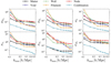 |
Fig. 8. Evolution of the marginalised constraint σθi on cosmological parameters {Ωm, Ωb, h, ns, σ8} and the sum of neutrino mass Mν with the maximum scale used for the Fisher analysis, kmax. σMν is in units of eV. |
An alternative quantity measuring the information carried by a statistic is given by the signal-to-noise ratio (S/N) that describes the reachable accuracy of the statistical measurement given the covariance matrix. In general, the S/N of a summary statistic s ∈ ℝn is defined as
 (16)
(16)
with Σ−1 being the corresponding precision matrix defined by Eq. (11). Figure 9 shows the evolution of the S/N for the matter and environment-dependent power spectra as a function of the maximum scale kmax. We again observe the flattening when kmax approaches non-linear scales at 0.25 h Mpc−1 for S/N(Pmm) (also reported in Angulo et al. 2008; Takahashi et al. 2010; Blot et al. 2015). This feature is also observed for some spectra in environments like filaments but at higher k values and all environment-dependent statistics reach a higher value of S/N, except for nodes. This latter saturates at an S/N 1.5 times smaller than the matter power spectrum at 0.5 h Mpc−1, making it the lowest value among all environments, which is coherent with the findings of the Fisher forecast. Void is the environment performing best individually over a wide range of scales but is overtaken by walls when kmax > 0.35 h Mpc−1. The shapes of the S/N evolution with kmax from the combination of environments also suggest that a further increase is possible when going to even smaller scales, kmax > 0.5 h Mpc−1, thanks to the breaking of degeneracies where the matter analysis is no longer able to improve. Quantitatively, the S/N obtained from the combination of environments is eight times higher than that from Pmm at kmax = 0.5 h Mpc−1.
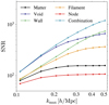 |
Fig. 9. Evolution of the signal-to-noise ratio S/N with kmax ∈ [0.11,0.5] Mpc h−1 for the several studied statistics: the matter power spectrum, the power spectrum computed in the cosmic web environments, and the combination of environment-dependent spectra. |
5. Discussion
The obtained results show that using summary statistics derived after segmenting the matter distribution into the different components of the cosmic web (voids, walls, filaments, and nodes) allows better leverage of cosmological parameters in real space than the matter power spectrum analysis. The derived statistics in individual environments also exhibit less correlations between Fourier modes, except for the highly non-linear environments that are nodes. Alternative approaches like the marked power spectrum and the wavelet scattering transform (WST) were employed in recent analyses of the very same sets of simulations and cosmological parameters by Massara et al. (2021) and Valogiannis & Dvorkin (2021), respectively. Alternatively, Bayer et al. (2021) propose an analysis using information from the halo mass function (HMF) and the void size function (VSF) in real space. All three analyses, together with ours, consider a maximum scale of kmax = 0.5 h Mpc−1 and can therefore be naturally compared. The constraints obtained from these various statistics are summarised in Table 3. The information contained in the power spectra bins in cosmic web environments provides the tightest constraints on Ωm, Ωb, h, and ns, and competitive values for constraints on Mν and σ8; however, these latter are both best constrained by the coefficients derived from the WST. Compared to the partial information from the extreme environments of voids and nodes obtained by Bayer et al. (2021), our environment-dependent statistics are able to tighten the constraints with improvement factors of {0.5, 4.1, 2.9, 3.1, 1.4, 1.7} on the parameters {Ωm, Ωb, h, ns, σ8, Mν}, hence performing better than the VSF + HMF statistic in all cases, except for Ωm.
Comparison of the marginalised 1-σ constraints obtained from different Fisher forecasts using different statistics.
It is however important to note that all these forecasts are performed in real space, and some statistics could be deeply affected by the redshift-space distortions breaking the density field isotropy. This is for instance the case of the WST, which requires adaption of the wavelets to be applied in this setting (Valogiannis & Dvorkin 2021), but also in our case, where the detection of the environment can be affected by the distortions, reducing the representative power of the environment-dependent statistics. Second, it should be noted that the analysis we propose is the only one including extra nuisance parameters related to the cosmic web classification, λth and σ𝒩, consequently artificially increasing the dimension of the parameter space and hence decreasing the constraints on the target parameters through additional degeneracies. As a fairer comparison, the last column of Table 3 shows the constraints we obtain when fixing the parameters of the classification method at their fiducial values. Finally, not only are the obtained values of the constraints important, but so is the physical interpretability of the coefficients encoding the field information. In that regard, the physical interpretability of the power spectra in cosmic web environments, being a simple two-point function, is straightforward, as well as the halo mass and void size functions.
6. Summary and conclusions
In this work, we carried out the first quantitative analysis of the cosmological information content of power spectra from the several cosmic web environments (nodes, filaments, walls, and voids). The derived statistics were computed from density fields associated with the environments identified through the eigenvalues of the Hessian matrix of the gravitational potential. Using the large suite of Quijote simulations, we performed a Fisher forecast by numerically estimating the partial derivatives and the covariance matrices of the extracted statistics in the non-linear regime with kmax = 0.5 h Mpc−1. We then compared the constraints on the cosmological parameters {Ωm, Ωb, h, ns, σ8, Mν} derived from the cosmic web environments to those from the analysis of the matter power spectrum, marginalising over the two parameters of the web-finder method. From this analysis in real space, we report that:
-
Environment-dependent spectra show different shape dependencies when varying cosmological parameters such as Mν, Ωm, and σ8 with respect to each other and to the matter power spectrum. These variations originate from the intrinsic differences in densities and hence evolution histories of each environment, where the observed structures at z = 0 are imprinted differently depending on the cosmology.
-
Power spectra in void, wall, and filament environments are less subject to mode coupling than the one computed from the matter for which overdense regions like nodes induce correlations between Fourier modes at small scales. As a result, voids and filaments for instance perform individually better than a matter power spectrum analysis for all cosmological parameters, except σ8.
-
The combination of power spectra in the environments leads to the breaking of some key degeneracies between parameters of the cosmological model which consequently tightens the constraints with improvement factors of {7.7, 4.5, 6.5, 15.7, 2.9, 15.2} on parameters {Ωm, Ωb, h, ns, σ8, Mν}, respectively, over the matter power spectrum. Such combination of spectra also yields an eight times higher S/N.
-
The constraints obtained from the combination of environments are superior to those obtained from the matter power spectrum for the whole range of maximum scales analysed in the range kmax ∈ [0.1,0.5] h Mpc−1.
-
For the maximum scale involved in the analysis, kmax = 0.5 h Mpc−1, the combination of environment-dependent spectra led to competitive (and better in some cases) constraints compared to other state-of-the-art numerical analyses relying on the same set of simulations, with the advantage of being easily interpreted.
-
The reported constraints are robust to variations of the two main parameters used to classify the environments, λth and σ𝒩. When varying these two parameters, the results are the same at the percentage level for Ωm, Ωb, and h, impacting mainly σ8, and Mν due to additional degeneracies.
In conclusion, we show that there is significantly more information contained in the density field when analysing the cosmic environments individually and using the combination of two-point statistics rather than when directly relying on the matter density field summarised by its power spectrum alone. The sizeable improvements in the constraints on all cosmological parameters brought by our environment-dependent analysis, even in the ideal case addressed in the present study, opens up the possibility to take advantage of the power spectra in environments for the optimal exploitation of future large galaxy redshift surveys such as the Dark Energy Spectroscopic Instrument (DESI, Levi et al. 2013) or Euclid (Laureijs et al. 2011). The present study however focuses on the real-space constraints obtained using information from cosmic web environments, both alone and combined. Applying this approach to observational data would consequently imply the use of biased tracers, analytical modelling of the spectra in the environments, and the inclusion of effects of redshift–space distortions. Physical observations will indeed provide us with biased tracers of the matter distribution, like halos or galaxies, instead of dark matter particles. Relying on such tracers would imply taking into account their relation to the matter distribution through notably the inclusion of additional nuisance parameters related to the so-called bias. These would both increase the dimension of the parameter space and induce additional degeneracies. Analytical modelling of the power spectrum as a function of the environments may be a complex endeavour even when relying on physically grounded web-finder methods such as the one used here, and in particular in the range of modes investigated here. Alternative approaches like simulation-based inference frameworks (see Leclercq 2018; Alsing et al. 2019; Cranmer et al. 2020) or emulators (as proposed in Heitmann et al. 2009, 2010, 2014; Lawrence et al. 2010) can be used to perform parameter estimation. Finally, observations are carried in redshift-space in which the peculiar velocities of matter tracers distort the spatial distribution, especially in dense regions. We still need to assess the information gain in the redshift space, where the multipole decomposition of the power spectrum already allows us to tighten the constraints on the matter component, and this will be the subject of a forthcoming paper (Bonnaire et al., in prep.).
The mass fractions are expressed here in terms of number of particles because they all have the same mass in the N-body simulations.
Acknowledgments
The authors thank the referee for their comments, all members of the ByoPiC team (https://byopic.eu/team) for useful discussions, as well as S. Codis, O. Hahn and M. Cautun for fruitful exchanges about this work. They also thank the Quijote team for making their data publicly available and particularly F. Villaescusa-Navarro for his help and availability regarding the Quijote suite. This research was supported by funding for the ByoPiC project from the European Research Council (ERC) under the European Union’s Horizon 2020 research and innovation program grant number ERC-2015-AdG 695561. A.D. was supported by the Comunidad de Madrid and the Complutense University of Madrid (Spain) through the Atracción de Talento program (Ref. 2019-T1/TIC-13298). T.B. acknowledges funding from the French government under management of Agence Nationale de la Recherche as part of the “Investissements d’avenir” program, reference ANR-19-P3IA-0001 (PRAIRIE 3IA Institute).
References
- Agarwal, N., Desjacques, V., Jeong, D., & Schmidt, F. 2021, JCAP, 2021, 021 [Google Scholar]
- Alam, S., Ata, M., Bailey, S., et al. 2017, MNRAS, 470, 2617 [Google Scholar]
- Allen, S. W., Evrard, A. E., & Mantz, A. B. 2011, ARA&A, 49, 409 [Google Scholar]
- Allys, E., Levrier, F., Zhang, S., et al. 2019, A&A, 629, A115 [NASA ADS] [CrossRef] [EDP Sciences] [Google Scholar]
- Allys, E., Marchand, T., Cardoso, J. F., et al. 2020, Phys. Rev. D, 102, 103506 [Google Scholar]
- Alpaslan, M., Robotham, A. S., Obreschkow, D., et al. 2014, MNRAS, 440, 1 [Google Scholar]
- Alsing, J., Charnock, T., Feeney, S., & Wandelt, B. 2019, MNRAS, 488, 4440 [Google Scholar]
- Angulo, R. E., Baugh, C. M., Frenk, C. S., & Lacey, C. G. 2008, MNRAS, 383, 755 [Google Scholar]
- Aragon-Calvo, M. A., Weygaert, R. V. D., & Jones, B. J. T. 2010a, MNRAS, 408, 2163 [CrossRef] [Google Scholar]
- Aragón-Calvo, M. A., Platen, E., Van De Weygaert, R., & Szalay, A. S. 2010b, ApJ, 723, 364 [CrossRef] [Google Scholar]
- Bahcall, N. A., & Fan, X. 1998, Am. Astron. Soc., 504, 1 [Google Scholar]
- Bahcall, N. A., Fan, X., & Cen, R. 1997, ApJ, 485, L53 [NASA ADS] [CrossRef] [Google Scholar]
- Barrow, J. D., Bhavsar, S. P., & Sonoda, D. H. 1985, MNRAS, 216, 17 [NASA ADS] [CrossRef] [Google Scholar]
- Bayer, A. E., Villaescusa-Navarro, F., Massara, E., et al. 2021, ApJ, 919, 24 [NASA ADS] [CrossRef] [Google Scholar]
- Beisbart, C., & Kerscher, M. 2000, ApJ, 545, 6 [NASA ADS] [CrossRef] [Google Scholar]
- Blot, L., Corasaniti, P. S., Alimi, J. M., Reverdy, V., & Rasera, Y. 2015, MNRAS, 446, 1756 [NASA ADS] [CrossRef] [Google Scholar]
- Bond, J. R., Kofman, L., & Pogosyan, D. 1996, Nature, 380, 603 [NASA ADS] [CrossRef] [Google Scholar]
- Bonjean, V., Aghanim, N., Salomé, P., Douspis, M., & Beelen, A. 2018, A&A, 609, A49 [NASA ADS] [CrossRef] [EDP Sciences] [Google Scholar]
- Bonjean, V., Aghanim, N., Douspis, M., Malavasi, N., & Tanimura, H. 2020, A&A, 638, A75 [NASA ADS] [CrossRef] [EDP Sciences] [Google Scholar]
- Bonnaire, T., Aghanim, N., Decelle, A., & Douspis, M. 2020, A&A, 637, A18 [NASA ADS] [CrossRef] [EDP Sciences] [Google Scholar]
- Bonnaire, T., Decelle, A., & Aghanim, N. 2021, IEEE Trans. Pattern Anal. Mach. Intell., [arXiv:2106.09035] [Google Scholar]
- Carron, J. 2013, A&A, 551, A88 [NASA ADS] [CrossRef] [EDP Sciences] [Google Scholar]
- Cautun, M., van de Weygaert, R., & Jones, B. J. 2013, MNRAS, 429, 1286 [NASA ADS] [CrossRef] [Google Scholar]
- Cautun, M., Weygaert, R. V. D., Jones, B. J. T., & Frenk, C. S. 2014, MNRAS, 441, 2923 [CrossRef] [Google Scholar]
- Chan, K. C., & Blot, L. 2017, Phys. Rev. D, 96, 023528 [NASA ADS] [CrossRef] [Google Scholar]
- Chen, Y. C., Ho, S., Freeman, P. E., Genovese, C. R., & Wasserman, L. 2015, MNRAS, 454, 1140 [CrossRef] [Google Scholar]
- Cheng, S., & Ménard, B. 2021, MNRAS, 8, 1 [Google Scholar]
- Cheng, S., Ting, Y.-S., Ménard, B., & Bruna, J. 2020, MNRAS, 499, 5902 [Google Scholar]
- Codis, S., Pogosyan, D., & Pichon, C. 2018, MNRAS, 479, 973 [Google Scholar]
- Cole, S., Percival, W. J., Peacock, J. A., et al. 2005, MNRAS, 362, 505 [Google Scholar]
- Cranmer, M., Sanchez-Gonzalez, A., Battaglia, P., et al. 2020, NeurIPS, accepted [arXiv:2006.11287] [Google Scholar]
- de Lapparent, V., Geller, M., & Huchra, J. 1987, ApJ, 302, L1 [Google Scholar]
- Doroshkevich, A. G., & Shandarin, S. F. 1978, Sov. Astron., 22, 653 [NASA ADS] [Google Scholar]
- Forero-Romero, J. E., Hoffman, Y., Gottlöber, S., Klypin, A., & Yepes, G. 2009, MNRAS, 396, 1815 [Google Scholar]
- Gil-Marín, H., Percival, W. J., Verde, L., et al. 2017, MNRAS, 465, 1757 [Google Scholar]
- Gruen, D., Friedrich, O., Amara, A., et al. 2016, MNRAS, 455, 3367 [Google Scholar]
- Gruen, D., Friedrich, O., Krause, E., et al. 2018, Phys. Rev. D, 98, 1 [CrossRef] [Google Scholar]
- Gualdi, D., Gil-marín, H., & Verde, L. 2021, JCAP, 2021, 008 [CrossRef] [Google Scholar]
- Hahn, C. H., & Villaescusa-Navarro, F. 2021, JCAP, 2021, 029 [CrossRef] [Google Scholar]
- Hahn, O., Porciani, C., Carollo, C. M., & Dekel, A. 2007, MNRAS, 375, 489 [NASA ADS] [CrossRef] [Google Scholar]
- Hahn, C. H., Villaescusa-Navarro, F., Castorina, E., & Scoccimarro, R. 2020, JCAP, 2020 [Google Scholar]
- Hamaus, N., Wandelt, B. D., Sutter, P. M., Lavaux, G., & Warren, M. S. 2014, Phys. Rev. Lett., 112, 1 [Google Scholar]
- Hamaus, N., Sutter, P. M., Lavaux, G., & Wandelt, B. D. 2015, JCAP, 2015 [Google Scholar]
- Hartlap, J., Simon, P., & Schneider, P. 2007, A&A, 464, 399 [NASA ADS] [CrossRef] [EDP Sciences] [Google Scholar]
- Heitmann, K., Higdon, D., White, M., et al. 2009, ApJ, 705, 156 [Google Scholar]
- Heitmann, K., White, M., Wagner, C., Habib, S., & Higdon, D. 2010, ApJ, 715, 104 [Google Scholar]
- Heitmann, K., Lawrence, E., Kwan, J., Habib, S., & Higdon, D. 2014, ApJ, 780, 111 [Google Scholar]
- Hockney, R. W., & Eastwood, J. W. 1981, Computer Simulation Using Particles (McGraw-Hill), 540 [Google Scholar]
- Holder, G., Haiman, Z., & Mohr, J. J. 2001, ApJ, 560, L111 [NASA ADS] [CrossRef] [Google Scholar]
- Jing, Y. P. 2005, ApJ, 620, 559 [NASA ADS] [CrossRef] [Google Scholar]
- Kaufman, G. 1967, Center for Operations Research and Econometrics, (Heverlee: Catholic University of Louvain), 6710, 44 [Google Scholar]
- Klypin, A., & Shandarin, S. 1983, MNRAS, 204, 891 [NASA ADS] [CrossRef] [Google Scholar]
- Kodwani, D., Alonso, D., & Ferreira, P. G. 2019, Open J. Astrophys., 2, 3 [NASA ADS] [CrossRef] [Google Scholar]
- Kreisch, C. D., Pisani, A., Carbone, C., et al. 2019, MNRAS, 488, 4413 [NASA ADS] [CrossRef] [Google Scholar]
- Kreisch, C. D., Pisani, A., Villaescusa-Navarro, F., et al. 2021, ApJ, submitted, [arXiv:2107.02304] [Google Scholar]
- Kuruvilla, J. 2022, A&A, 660, A113 [NASA ADS] [CrossRef] [EDP Sciences] [Google Scholar]
- Kuruvilla, J., & Aghanim, N. 2021, A&A, 653, A130 [NASA ADS] [CrossRef] [EDP Sciences] [Google Scholar]
- Laureijs, R., Amiaux, J., Arduini, S., et al. 2011, ArXiv e-prints [arXiv:1110.3193] [Google Scholar]
- Lavaux, G., & Wandelt, B. D. 2012, ApJ, 754, 109 [NASA ADS] [CrossRef] [Google Scholar]
- Lawrence, E., Heitmann, K., White, M., et al. 2010, ApJ, 713, 1322 [Google Scholar]
- Leclercq, F. 2018, Phys. Rev. D, 98, 1 [CrossRef] [Google Scholar]
- Lee, J., & Park, D. 2009, ApJ, 696, L10 [NASA ADS] [CrossRef] [Google Scholar]
- Levi, M., Bebek, C., Beers, T., et al. 2013, ArXiv e-prints [arXiv:1308.0847] [Google Scholar]
- Libeskind, N. I., van de Weygaert, R., Cautun, M., et al. 2017, MNRAS, 473, 1195 [Google Scholar]
- Malavasi, N., Arnouts, S., Vibert, D., et al. 2017, MNRAS, 465, 3817 [Google Scholar]
- Malavasi, N., Langer, M., Aghanim, N., Galárraga-Espinosa, D., & Gouin, C. 2022, A&A, 658, A113 [NASA ADS] [CrossRef] [EDP Sciences] [Google Scholar]
- Mallat, S. 2012, Commun. Pure Appl. Math., 65, 1331 [CrossRef] [Google Scholar]
- Martizzi, D., Vogelsberger, M., Artale, M. C., et al. 2019, MNRAS, 486, 3766 [Google Scholar]
- Marulli, F., Veropalumbo, A., Sereno, M., et al. 2018, A&A, 620, A1 [NASA ADS] [CrossRef] [EDP Sciences] [Google Scholar]
- Massara, E., Villaescusa-Navarro, F., Viel, M., & Sutter, P. M. 2015, JCAP, 2015, 018 [Google Scholar]
- Massara, E., Villaescusa-Navarro, F., Ho, S., Dalal, N., & Spergel, D. N. 2021, Phys. Rev. Lett., 126, 1 [CrossRef] [Google Scholar]
- Mueller, E. M., Bernardis, F. D., Bean, R., & Niemack, M. D. 2015, ApJ, 808, 47 [NASA ADS] [CrossRef] [Google Scholar]
- Naidoo, K., Whiteway, L., Massara, E., et al. 2020, MNRAS, 491, 1709 [NASA ADS] [CrossRef] [Google Scholar]
- Naidoo, K., Massara, E., & Lahav, O. 2022, MNRAS, accepted, [arXiv:2111.12088] [Google Scholar]
- Paillas, E., Cai, Y. C., Padilla, N., & Sánchez, A. G. 2021, MNRAS, 505, 5731 [NASA ADS] [CrossRef] [Google Scholar]
- Peloso, M., Pietroni, M., Viel, M., & Villaescusa-Navarro, F. 2015, JCAP, 2015, 1 [Google Scholar]
- Pereyra, L. A., Sgró, M. A., Merchán, M. E., Stasyszyn, F. A., & Paz, D. J. 2020, MNRAS, 499, 4876 [Google Scholar]
- Philcox, O. H. 2021, MNRAS, 501, 4004 [NASA ADS] [CrossRef] [Google Scholar]
- Pisani, A., Sutter, P.M., Hamaus, N., et al. 2015, Phys. Rev. D, 92, 1 [Google Scholar]
- Planck Collaboration VI. 2020, A&A, 641, A6 [NASA ADS] [CrossRef] [EDP Sciences] [Google Scholar]
- Salvati, L., Douspis, M., & Aghanim, N. 2018, A&A, 614, A13 [NASA ADS] [CrossRef] [EDP Sciences] [Google Scholar]
- Schmittfull, M. M., Regan, D. M., & Shellard, E. P. 2013, Phys. Rev. D, 88, 1 [Google Scholar]
- Schuster, N., Hamaus, N., Pisani, A., et al. 2019, JCAP, 2019, 055 [Google Scholar]
- Sefusatti, E., Crocce, M., Pueblas, S., & Scoccimarro, R. 2006, Phys. Rev. D, 74, 023522 [NASA ADS] [CrossRef] [Google Scholar]
- Sefusatti, E., Crocce, M., Scoccimarro, R., & Couchman, H. M. 2016, MNRAS, 460, 3624 [NASA ADS] [CrossRef] [Google Scholar]
- Sheth, R. K., Connolly, A. J., & Skibba, R. 2005, ArXiv e-prints [arXiv:astro-ph/0511773] [Google Scholar]
- Skrutskie, M. F., Cutri, R. M., Stiening, R., et al. 2006, AJ, 131, 1163 [NASA ADS] [CrossRef] [Google Scholar]
- Sousbie, T. 2011, MNRAS, 414, 350 [NASA ADS] [CrossRef] [Google Scholar]
- Springel, V. 2005, MNRAS, 364, 1105 [Google Scholar]
- Stoica, R. S., Martínez, V. J., & Saar, E. 2007, J. R. Stat. Soc. Ser. C: Appl. Stat., 56, 459 [CrossRef] [Google Scholar]
- Stoyan, D. 1984, Math. Naschr., 197 [CrossRef] [Google Scholar]
- Takahashi, R., Yoshida, N., Takada, M., et al. 2010, ApJ, 726, 7 [Google Scholar]
- Tempel, E., Stoica, R. S., Kipper, R., & Saar, E. 2016, Astron. Comput., 16, 17 [NASA ADS] [CrossRef] [Google Scholar]
- Tinker, J. L., Sheldon, E. S., Wechsler, R. H., et al. 2012, ApJ, 745, 16 [NASA ADS] [CrossRef] [Google Scholar]
- Uhlemann, C., Friedrich, O., Villaescusa-Navarro, F., Banerjee, A., & Codis, S. 2020, MNRAS, 495, 4006 [NASA ADS] [CrossRef] [Google Scholar]
- Valogiannis, G., & Dvorkin, C. 2021, ArXiv e-prints [arXiv:2108.07821] [Google Scholar]
- van de Weygaert, R., & Platen, E. 2011, Int. J. Mod. Phys.: Conf. Ser., 1, 41 [NASA ADS] [CrossRef] [Google Scholar]
- Villaescusa-Navarro, F., Vogelsberger, M., Viel, M., & Loeb, A. 2013, MNRAS, 431, 3670 [NASA ADS] [CrossRef] [Google Scholar]
- Villaescusa-Navarro, F., Marulli, F., Viel, M., et al. 2014, JCAP, 2014, 011 [CrossRef] [Google Scholar]
- Villaescusa-Navarro, F., Hahn, C. H., Massara, E., et al. 2020, ApJ, 250, 2 [NASA ADS] [Google Scholar]
- Wang, P., Kang, X., Libeskind, N. I., et al. 2020, New Astron., 80, 101405 [NASA ADS] [CrossRef] [Google Scholar]
- White, M. 2016, JCAP, 11, 057 [CrossRef] [Google Scholar]
- Yankelevich, V., & Porciani, C. 2019, MNRAS, 483, 2078 [NASA ADS] [CrossRef] [Google Scholar]
- York, D. G., Adelman, J., Anderson, J., et al. 2000, ApJ, 120, 1579 [CrossRef] [Google Scholar]
- Zel’dovich, Y. B. 1970, A&A, 5, 84 [NASA ADS] [Google Scholar]
Appendix A: Stability and convergence analysis
In the Fisher forecast, we resort to numerical estimations of the precision matrices defined in Eq. (11) but also of the derivatives from Eq. (12) and (13). To avoid biased results induced by a non-convergence of these quantities, it is essential to check the stability of the derived constraints under reduction of both Nfid, the number of simulations used to compute the covariances, and Nderiv, the number of simulations for the derivatives. We focus here on the convergence of the constraints σθi derived in all setups, from individual environments with 40 Fourier bins or from the combination of power spectra yielding the maximum total length among all the studied statistical summaries with n = 160. We note that the convergence of the matter power spectrum in Quijote simulations is already studied in Villaescusa-Navarro et al. (2020). In Fig. A.1, we show how the maximum deviation of marginalised constraints behaves when varying Nfid in the upper panel and Nderiv in the lower one. We plot, for each considered statistic, the evolution of the maximum deviation over all cosmological parameters
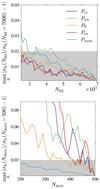 |
Fig. A.1. Convergence analysis of the numerical precision matrix as a function of Nfid with fixed Nderiv = 500 (upper panel) and derivatives as a function of Nderiv with fixed Nfid = 7000 (lower panel) for the combined spectra statistics Pcomb. The grey area shows the 2% agreement area. |
 (A.1)
(A.1)
with N being either Nfid or Nderiv and Nmax respectively taking values 7000 and 500. For all the individual environments and their combination, convergence at a ±2% level is obtained when Nfid ∼ 4500 for the computation of the covariance matrix. Individually, the constraints from the several statistics reach 5% convergence when Nderiv ≤ 400 for all environments except walls for which the 5% level is obtained around 450 simulations. However, convergence of the derivatives is obtained at the percentage level for Pcomb when Nderiv ≃ 300, highlighting the good convergence properties of this statistic and excluding any bias induced by numerical instabilities in the computation of Fisher constraints for the combination of spectra.
Appendix B: Gaussianity of the statistics
When deriving the Fisher matrices in Eq. (10), we assumed the distribution of the statistics s to be Gaussian, expressed through Eq. (7). To quantify any deviation from Gaussianity which could lead to biased estimation of errors, we report in Fig. B.1 the skewness and excess kurtosis distributions for each k bin for all the computed power spectra. At large scales, the small number of modes available to compute the averages of Eq. (5) creates significant non-Gaussianities for all spectra. As a result of the central limit theorem, at higher values of k, there are more modes for the estimators to be averaged over leading the Gaussian hypothesis to be more accurate. Still, some spectra, mainly Pmm and Pnn, show deviations from the Gaussian hypothesis at small k with a higher value of the skewness compared to other spectra. The impact of these non-Gaussian signatures is however limited in our analysis because we mostly focus on the gains of our statistics with respect to the matter power spectrum which already exhibits the same features.
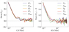 |
Fig. B.1. Skewness (left panel) and excess kurtosis (right panel) distributions for each k bin of the power spectra. In both plots, the dashed grey horizontal line denotes the zero value. |
Appendix C: Constraints with fixed segmentation parameters
In the main text, the presented results show the cosmological constraints obtained on Ωm, Ωb, h, ns, σ8 and Mν in Table 2 when marginalising over the two parameters of the T-web formalism used to identify the environments, namely λth and σ𝒩. As expected, when fixing these at their fiducial values, respectively 0.3 and 2 h/Mpc, the constraints are tighter, as presented in Table C.1. This especially occurs for the σ8 and Mν parameters, while the others remain unchanged.
Marginalised 1-σ constraints obtained from the power spectrum in different environments for all cosmological parameters when fixing the nuisance parameters to their fiducial values, namely λth = 0.3 and σ𝒩 = 2 Mpc/h. σMν is in units of eV.
All Tables
Cosmic web classification rules in the cell x depending on the eigenvalues λ1 ≤ λ2 ≤ λ3 of the tidal tensor.
Marginalised 1-σ constraints obtained from the power spectrum in different environments for all cosmological parameters in real space and considering λth and σ𝒩 as nuisance parameters.
Comparison of the marginalised 1-σ constraints obtained from different Fisher forecasts using different statistics.
Marginalised 1-σ constraints obtained from the power spectrum in different environments for all cosmological parameters when fixing the nuisance parameters to their fiducial values, namely λth = 0.3 and σ𝒩 = 2 Mpc/h. σMν is in units of eV.
All Figures
|
Fig. 1. Overdensity fields computed in the different environments. From top to bottom: set of five 2.77 Mpc h−1 depth slices showing the fields δm, δv, δf, δw, and δn, respectively. Overdensity fields in cosmic web environments are computed from the T-web classification of particles and are normalised such that δm = ∑αfαδα. |
| In the text | |
|
Fig. 2. Averaged mass fractions ⟨fα⟩ in the different cosmic web environments for distinct values of |
| In the text | |
|
Fig. 3. Ratios between mass fractions in the cosmic web environments and mass fractions obtained with fiducial cosmology for an eigenvalue threshold of |
| In the text | |
|
Fig. 4. Top panel: real-space normalised power spectra |
| In the text | |
|
Fig. 5. Correlation coefficients Cij for the matter power spectrum (top) and the power spectra in the several environments (bottom). Each submatrix goes from k = 0.1 h Mpc−1 to k = 0.5 h Mpc−1. |
| In the text | |
|
Fig. 6. Partial derivatives ∂Pαα(k)/∂θi for the different environmental auto-spectra and for each studied parameter {Ωm, Ωb, h, ns, σ8, Mν}. Dashed (respectively solid) lines correspond to negative (respectively positive) values of the derivative. The grey area depicts the range of k > kmax excluded from the analysis. |
| In the text | |
|
Fig. 7. 1σ confidence ellipses for all the pairs of cosmological (Ωm,Ωb,h,ns,σ8,Mν) and nuisance (λth) parameters obtained from the matter power spectrum, or the spectra from the different environments and their combination in real space. The normalised probability density function for each parameter is shown on the diagonal. |
| In the text | |
|
Fig. 8. Evolution of the marginalised constraint σθi on cosmological parameters {Ωm, Ωb, h, ns, σ8} and the sum of neutrino mass Mν with the maximum scale used for the Fisher analysis, kmax. σMν is in units of eV. |
| In the text | |
|
Fig. 9. Evolution of the signal-to-noise ratio S/N with kmax ∈ [0.11,0.5] Mpc h−1 for the several studied statistics: the matter power spectrum, the power spectrum computed in the cosmic web environments, and the combination of environment-dependent spectra. |
| In the text | |
|
Fig. A.1. Convergence analysis of the numerical precision matrix as a function of Nfid with fixed Nderiv = 500 (upper panel) and derivatives as a function of Nderiv with fixed Nfid = 7000 (lower panel) for the combined spectra statistics Pcomb. The grey area shows the 2% agreement area. |
| In the text | |
|
Fig. B.1. Skewness (left panel) and excess kurtosis (right panel) distributions for each k bin of the power spectra. In both plots, the dashed grey horizontal line denotes the zero value. |
| In the text | |
Current usage metrics show cumulative count of Article Views (full-text article views including HTML views, PDF and ePub downloads, according to the available data) and Abstracts Views on Vision4Press platform.
Data correspond to usage on the plateform after 2015. The current usage metrics is available 48-96 hours after online publication and is updated daily on week days.
Initial download of the metrics may take a while.