| Issue |
A&A
Volume 674, June 2023
|
|
|---|---|---|
| Article Number | A150 | |
| Number of page(s) | 11 | |
| Section | Cosmology (including clusters of galaxies) | |
| DOI | https://doi.org/10.1051/0004-6361/202245626 | |
| Published online | 16 June 2023 | |
Cosmology with cosmic web environments
II. Redshift-space auto and cross-power spectra
1
Laboratoire de Physique de l’École normale supérieure, ENS, Université PSL, CNRS, Sorbonne Université, Université Paris Cité, 75005 Paris, France
e-mail: This email address is being protected from spambots. You need JavaScript enabled to view it.
2
Université Paris-Saclay, CNRS, Institut d’Astrophysique Spatiale, 91405 Orsay, France
3
Université Paris-Saclay, TAU team INRIA Saclay, CNRS, Laboratoire Interdisciplinaire des Sciences du Numérique, 91190 Gif-sur-Yvette, France
4
Departamento de Física Teórica I, Universidad Complutense, 28040 Madrid, Spain
Received:
6
December
2022
Accepted:
19
April
2023
Abstract
Degeneracies among parameters of the cosmological model are known to drastically limit the information contained in the matter distribution. In the first paper of this series, we show that the cosmic web environments, namely the voids, walls, filaments and nodes, can be used as leverage to improve the real-space constraints on a set of six cosmological parameters, including the summed neutrino mass. Following up on these results, we propose to investigate the extent to which constraints can be obtained with environment-dependent power spectra in redshift space where the velocities add information to the standard two-point statistics by breaking the isotropy of the matter density field. A Fisher analysis based on a set of thousands of Quijote simulations allows us to conclude that a combination of power spectra computed in several cosmic web environments is able to break some degeneracies. Compared to the matter monopole and quadrupole information alone, the combination of environment-dependent spectra improves constraints on key parameters such as the matter density and the summed neutrino mass by up to a factor of 5.5. Additionally, while the information contained in the matter statistic quickly saturates at mildly non-linear scales in redshift space, a combination of power spectra from different environments appears to be a rich source of information that can be used to improve the constraints at all the studied scales from 0.1 to 0.5 h Mpc−1 and suggests that further improvements could be attainable at even finer scales.
Key words: cosmology: theory / large-scale structure of Universe / cosmological parameters
© The Authors 2023
 Open Access article, published by EDP Sciences, under the terms of the Creative Commons Attribution License (https://creativecommons.org/licenses/by/4.0), which permits unrestricted use, distribution, and reproduction in any medium, provided the original work is properly cited.
This article is published in open access under the Subscribe to Open model. This email address is being protected from spambots. You need JavaScript enabled to view it. to support open access publication.
1. Introduction
The spatial distribution of matter in the Universe is a powerful probe to constrain cosmological parameters (see e.g. Totsuji & Kihara 1969; Peacock et al. 2001; Eisenstein et al. 2005; Mandelbaum et al. 2013; Alam et al. 2017a; Hildebrandt et al. 2017; D’Amico et al. 2020; Colas et al. 2020; Ivanov et al. 2020), test the theory of gravity (Alam et al. 2017b, 2021; Jullo et al. 2019; Blake et al. 2020), and improve our understanding of dark matter and dark energy (Abbott et al. 2019; Drlica-Wagner et al. 2019). All these possibilities have led numerous collaborations over the past decades to initiate a race to map the largest number of galaxies in the sky with the highest possible accuracy. Stage IV of these galaxy redshift surveys – notably the Dark Energy Spectroscopic Instrument1 (DESI Collaboration 2016), Euclid2 (Laureijs et al. 2011) and the Nancy Grace Roman space telescope3 (Spergel et al. 2015) – promises an unprecedented amount of data, enabling, among other things, the most accurate estimate of cosmological parameters to date. However, these expected observational achievements must be accompanied by appropriate theoretical and numerical advances. Although widely used in most analyses because of its simplicity, it is well-known that the power spectrum (or equivalently the two-point correlation function), for example, is not a sufficient summary statistic when it comes to non-Gaussian fields such as the late-time distribution of matter in the Universe. Another caveat that must be taken into account when using the matter power spectrum for cosmological analyses is the degeneracies among parameters of the Λ cold dark matter (ΛCDM) model, which have a similar impact over a wide range of scales, limiting the information one can extract from the model.
Over recent years, several strategies have been proposed to fight the degeneracies and go beyond simple power spectrum analyses in order to optimally exploit the matter distribution. These have included information coming from higher-order statistics (Hahn et al. 2020; Hahn & Villaescusa-Navarro 2021; Gualdi et al. 2021; Philcox & Ivanov 2022), velocities (Mueller et al. 2015; Kuruvilla & Aghanim 2021; Kuruvilla 2022), marked power spectra (Massara et al. 2021, 2022), wavelet-based statistics (Allys et al. 2020; Cheng et al. 2020; Cheng & Ménard 2021; Valogiannis & Dvorkin 2022a,b; Eickenberg et al. 2022; Wang & He 2022; Wang et al. 2022), split densities (Uhlemann et al. 2020; Paillas et al. 2021, 2023), partial or total cosmological environments (Kreisch et al. 2022; Bayer et al. 2021; Bonnaire et al. 2021; Woodfinden et al. 2022), or from the minimum spanning tree (Naidoo et al. 2020, 2022). While the recent literature abounds in analyses and forecasts designed to identify the optimal statistic in real space, only a few studies have addressed the problem in the space in which the data are actually collected, namely redshift space. It is nonetheless well-known that the additional information carried by velocities coming into play in this space is non-negligible and leads to considerable improvement of the cosmological constraints derived from the standard matter statistics.
The real-space results presented in Bonnaire et al. (2021) demonstrated the ability of simple two-point statistics derived in the separate cosmic web environments (voids, walls, filaments, and nodes) to break key degeneracies in the cosmological model, consequently enabling the improvement of constraints on all the parameters compared to those derived from the matter power spectrum. In the present study, we extended our analysis of the constraints obtained by the combination of power spectra computed in several environments when considering redshift-space distortions (RSDs). In particular, we investigated how the combination of environment-dependant spectra in this space can improve the cosmological constraints, and how these latter compare to the real-space case without correcting the distortions at all. To this end, we performed a Fisher forecast of the constraints using numerous simulations with varying cosmological parameters in order to numerically assess the information contained in our statistics on the cosmological parameters. The paper is organised such that Sect. 2 presents the Quijote suite of simulations and the methodology used to extract the cosmic web environments while Sect. 3 introduces the power-spectra estimation in redshift space and in the cosmic web environments. Section 4 then presents the forecast constraints in redshift space but also compares these with the real space findings reported in Bonnaire et al. (2021). Finally, Sect. 5 provides a discussion of the obtained results in view of the recent literature, gives perspectives for future steps towards the use of this kind of analysis in observational setups, and also contains a summary and our conclusions.
2. Data and methodology
2.1. The Quijote simulations
Our analysis relies on the Quijote4 (Villaescusa-Navarro et al. 2020) suite, which provides a set of 44 100 N-body simulations. With realisations of more than 7000 cosmological models, this large suite of simulations was precisely designed to perform statistical analyses and train machine learning algorithms. Initialised with the second-order Lagrangian perturbation theory (or Zel’dovich approximation in case of massive neutrino simulations), N = 5123 dark matter particles (and 5123 neutrinos in case there are) are evolved forward in time in an L = 1 h Gpc−1 size box from redshift z = 127 to z = 0. There are 15 000 simulations available at the fiducial cosmology, which is assumed to be a flat ΛCDM cosmology with parameters Ωm = 0.3175, Ωb = 0.049, h = 0.6711, ns = 0.9624, σ8 = 0.834, and Mν = 0, with Mν being the summed neutrino mass. For each cosmological parameter, 500 simulations are then individually computed with a fixed increase and decrease, dΩm = ±0.010, dΩb = ±0.002, dh = ±0.020, dns = ±0.020, and dσ8 = ±0.015. Because Mν is a positive quantity, the Quijote suite provides four positive variations of this parameter with Mν = ∑mν = {0.1, 0.2, 0.4} eV.
2.2. Cosmic web classification
Among the many possible definitions of the cosmic web environments proposed in the literature (see Stoica et al. 2007; Aragon-Calvo et al. 2010; Cautun et al. 2013; Sousbie 2011; Tempel et al. 2014; Bonnaire et al. 2020, 2022, to name only a few), we resort to an implementation of the T-Web algorithm (Hahn et al. 2007; Forero-Romero et al. 2009). We summarise the general steps of the classification below. We first start by computing a smooth density field ρ(x) based on the discrete set of particles by means of a B-spline interpolation of order four over an  three-dimensional grid. The T-Web formulation relies on the tidal tensor T(x), the second derivative of the gravitational potential, itself computed from ρ(x), and the Poisson equation. Each of the grid cells x is classified as either void, wall, filament, or node depending on the eigenvalues of the tidal tensor. More precisely, a cell x is in a void if the three eigenvalues are below λth; in a wall if only two are below λth; in a filament if only one is below λth; and in a node if none are below this threshold. From the classification of the
  cells of the density field, we propagate the environments at the particle level, enabling the computation of four individual overdensity fields, δv, δw, δf, and δn, where the subscripts refer to void, wall, filament, and node, respectively. These fields are all linked to the full matter overdensity field δm by the linear combination δm = ∑α ∈ {v, w, f, n}fαδα, where fα = Nα/N denotes the mass fraction5 of the environment α.
The classification scheme relies on three parameters. The first two are related to the coarseness of the smooth gravitational potential estimation,  , the number of grid cells, and σ𝒩, the scale of the Gaussian with which the potential is being smoothed before performing the classification. The last parameter, λth, corresponds to the threshold used for the classification of the environments based on the amplitudes of the eigenvalues of the tidal tensor. In Bonnaire et al. (2021), we explored the impact of the parameters and ultimately set
  cells and a value of σ𝒩 = 2 h Mpc−1 for the smoothing scale. This yields an effective smoothing of 3.4 h Mpc−1, which corresponds to the physical size of the structures, such as galaxy clusters or filament widths (see Cautun et al. 2014). The eigenvalue threshold is set to λth = 0.3 in order to obtain a cosmic web that is consistent with the use of such a methodology in the literature and in which the voids start to percolate (see e.g. Hahn et al. 2007; Martizzi et al. 2019; Libeskind et al. 2017; Bonnaire et al. 2021). We refer the reader to the first paper of the series (Bonnaire et al. 2021) for details on the analysis and assessment of these choices of parameter values.
3. Redshift space
3.1. Redshift-space distortions
When dealing with observational data, the redshift is used as a measure of the distance. However, this quantity is the combination of the proper motion of the source due to its peculiar velocity, v, and the expanding Universe. Considering xr, the position of a source in the comoving space, xs, its position in the redshift space, and  , a unit vector in the line of sight (LoS) direction, we can obtain the mapping relation
 (1)
(1)
where a is the scale factor and H the Hubble constant. This shift distorts the spatial distribution of the tracers, and is known as redshift-space distortion (RSD), which leads to two dominant effects: The first is the finger-of-God (FoG) effect (Jackson 1972), which makes overdense clustered regions appear elongated in the LoS direction due to the high velocity of the sources, and the second, observed on larger scales, is a squashing effect of dense regions along the LoS known as the Kaiser effect (Kaiser 1987).
While Bonnaire et al. (2021) focused on the information content of power spectra in cosmic web environments computed in real space, with the current work we propose to investigate the information in redshift space, which is therefore expected to more closely resemble observations. To do so, we mimic the effect of RSDs in each individual simulation by displacing all particles (dark matter particles and neutrinos if any) according to Eq. (1) along one Cartesian axis of the box, and therefore assume that the plane-parallel approximation holds.
3.2. Power-spectra estimation in redshift-space
In a general manner, the cross-power spectrum is defined as the covariance of Fourier transformed overdensity fields δα and δβ and is given by
 (2)
(2)
where  , which is the angle with the line of sight, Pαβ(k, μ) is the 2D power spectrum obtained by binning both in k and μ, and ℒℓ are the Legendre polynomials. In real space, the isotropy of the density field implies that all the ℓ > 0 terms cancel out, leaving the monopole alone to carry all the information. In redshift space, the peculiar velocities of particles induce a dependence of the power spectrum on the LoS, which leads to the breaking of the density field isotropy and consequently spreads the power over the multipoles ℓ. Throughout the present paper, we write Pαβ(k) to denote the cross- or auto-spectra monopole in real space and keep the subscript s to denote statistics computed in redshift space, together with the superscript ℓ, which refers to the multipole. To characterise spectra in redshift space, we rely on the three first non-zero multipoles, namely
  , and
, and  , respectively, which are called the monopole, quadrupole, and hexadecapole. These ℓ ≤ 4 orders are the only non-vanishing moments in the linear approximation of the distortions and encode the full 2D information at linear scales (Kaiser 1987). The corresponding Legendre polynomials are
 (3)
(3)
Similarly to Bonnaire et al. (2021), we deconvolve the fields δα before estimating the power spectra to remove the biasing effect in the estimation introduced by the smoothing of the fourth-order B-spline interpolation to obtain the density fields. For additional robustness to any bias provoked by aliasing effects, the maximum Fourier bin, which we set at kmax = 0.5 h Mpc−1 by default, is below half of the Nyquist frequency defined as kNyq = πNg/L = 0.57 h Mpc−1.
3.3. Cosmic web environments and redshift space
Figure 1 shows the ratios between the real-space and redshift-space monopoles obtained from the average of 7000 fiducial simulations. It is worth mentioning that the spectra are not weighted by the mass fraction of the environments, which in particular means that the matter multipoles cannot be recovered by summing the auto- and cross-spectra obtained in the environments, that is,  . As expected, all the spectra are boosted at large scales (small k values) due to the coherent motion of matter escaping from voids and moving towards dense regions because of the Kaiser effect. On the other hand, a decrease in power is observed at smaller scales where the FoG effect dominates, spreading particles initially residing in spherical overdensities along the line of sight. FoG mostly impacts the node environment where the highest velocities are found. Beyond the shape of the spectra in redshift space, the individual impact of each cosmological parameter is also different, as illustrated in Fig. 2. As an example, decreasing σ8 does not imply a simple shift of the matter power spectrum monopole in redshift space but is boosting the power at small scales (large k values) due to the FoG effect. This is illustrated by the dashed lines of the top-left panel, which show the monopole residuals
  with θi being either
  ,
,  , or
, or  . These effects can then cause degeneracies between cosmological parameters. It has been shown for instance that the effect of massive neutrinos can be mimicked by a decrease in σ8 on the redshift-space monopole at small scales k > 0.1 h Mpc−1 (see e.g. Villaescusa-Navarro et al. 2018; Hahn et al. 2020; Bayer et al. 2022), which in turn has a similar impact to a decrease in Ωm. Comparing with the bottom-left panels of Fig. 2, we see that the monopoles computed in the cosmic web environments have various dependencies when decreasing the three parameters. Consequently, a change in σ8 can no longer be reproduced by increasing the summed neutrino mass, illustrating the breaking of degeneracies that we expect by analysing the several environments separately. However, the anisotropic nature of the matter density field in redshift space leads to nonzero ℓ > 0 multipoles that already have various shapes when varying these parameters, as illustrated in the upper right panel of Fig. 2 for ℓ = 2. This suggest that combining the two first multipoles of the matter density field should allow us to break some degeneracies already. However, the measurements of the multipoles are noisier when going to larger ℓ and it might be interesting to measure the achievable accuracy of the environment monopoles only. The right-bottom panels also show that the environments themselves have different shapes for ℓ = 2, suggesting further potential for imposing tighter constraints using the statistics drawn from combining the four monopoles and the four quadrupoles derived in the different environments.
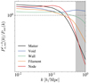 |
Fig. 1. Ratio between the redshift-space and real-space monopoles computed in the cosmic web environments. The grey shaded region shows the scales k > 0.5 h Mpc−1, which are unused in this analysis. |
The effects of the distortions are also clearly rooted in the classification itself, where we expect for instance the FoG to lead to a leakage of some cells classified in nodes in real space to filaments in redshift space. These effects are quantified in Table 1, which reports the confusion matrix averaged over ten simulations at fiducial cosmology when considering the real-space classification as the ground truth. The non-diagonal terms of this matrix therefore correspond to the fraction of change in the environment classification when going from real to redshift space and a perfect match would lead to the identity matrix. The matrix shows for instance that 36.7% of the particles classified in nodes in real space are found in filaments when the classification is performed in redshift space. We note that the leakage mostly occurs between one environment and another of directly higher local dimension (i.e. voids to walls, walls to filaments, and filaments to nodes), while very little leakage occurs between environments of higher dimensions. We interpret this effect as a result of our plane-parallel approximation, which forces the distortions to occur along one spatial axis only. It is worth underlining that, apart from nodes, the classification is quite stable to the distortions, with about 80% of the particles in each environment (voids, walls, and filaments) keeping the same classification in real and redshift spaces.
Averaged confusion matrix obtained from ten boxes of the Quijote simulations with the fiducial cosmology when considering the absence of RSD as a ground truth.
4. Cosmological constraints
To quantify the amount of information carried by the spectra computed in the cosmic web environments, we make use of a Fisher analysis (details can be found in Appendix A). Briefly, this latter allows us to derive a lower bound on the constraints that one would achieve when relying on a given statistic, in our case either the spectra in the cosmic web environments or the full matter power spectrum. The derivation of the constraints mostly relies on two elements, both of which we derive numerically from the Quijote simulations: (i) the covariance matrix between Fourier amplitudes and (ii) the derivatives of the statistic with respect to the six cosmological parameters Ωm, Ωb, h, ns, σ8, and Mν. The covariance matrices used in the Fisher forecast are shown in Appendix B.
The first row of Table 2 gives the constraints obtained from the real-space matter power spectrum presented in Bonnaire et al. (2021), while the second and third rows show the redshift-space constraints from the matter monopole  and the combination of the monopole and quadrupole
  , respectively. It is particularly striking that the redshift-space constraints obtained from just the monopole allow us to improve those in real space for Ωm by a factor of up to 12 and those for Mν by a factor of up to 2.4. These gains even reach 21.1 and 10.5, respectively, when adding the information of the quadrupole in the
  statistic. Such results are expected when moving from real to redshift space due to the additional velocity information coming into play in the breaking of the density field isotropy. It is also interesting to note that only σσ8 and σMν are drastically reduced when adding the quadrupole information to the matter monopole, while the error on other parameters remains roughly the same, quantifying the expected breaking of degeneracy between these two parameters discussed in Sect. 3.3 and illustrated in the top panels of Fig. 2.
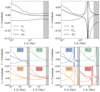 |
Fig. 2. Residuals of the matter monopole (upper left panel) or quadrupole (upper right panel) and environment-dependent monopoles (lower left panel) or quadrupoles (lower right panel) when varying either σ8, Ωm, or Mν. Residuals are defined as |


Marginalised 1σ constraints obtained from the analysis of power-spectra monopoles and quadrupoles computed in the different environments for all cosmological parameters.
Concerning the environment-dependent spectra, we report the following in rows four to six of Table 2:
– Using the combination of environment monopoles (fourth line of Table 2) already provides tighter constraints than the combination of the first two multipoles of the full matter density field,  (third line of Table 2), with improvement factors of up to 2.1 and 1.7 for ns and Mν, respectively.
– Adding the ℓ = 2 information brings down the constraints to even lower values with improvement factors of {1.7, 1.4, 1.8, 2.4, 1, 2.7} on cosmological parameters {Ωm, Ωb, h, ns, σ8, Mν} with respect to the matter analogue in redshift space, as shown in the fifth row of Table 2. Similarly to what is observed in the matter case, adding up the ℓ = 2 information mostly breaks the degeneracy on Mν without greatly impacting the set of other parameters.
– The constraints imposed by the combination of environment statistics highly depend on the maximum scale of the spectra included in the analysis. Many panels of Fig. 3 indeed indicate that the matter monopole+quadrupole saturates at mildly non-linear scales, a feature already exhibited in the real space analysis from Bonnaire et al. (2021) and previously pointed out by Takahashi et al. (2010), Blot et al. (2015), Chan & Blot (2017). This saturation, which is mainly due to the degeneracies among parameters of the cosmological model, is not observed for the combination of environment-dependent spectra, and is a particular encouragement for us to push the limiting scale of the analyses further in order to fully capitalise on the potential of the cosmic web split.
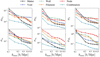 |
Fig. 3. Evolution of the marginalised constraint σθi given by |

– Unlike the real-space case, the improvement factors of the individual environments are below one for all parameters when kmax = 0.5 h Mpc−1 (see Table C.1). This observation is not true at all scales, as illustrated by Fig. 3, where the environments perform individually better than the matter statistics when restricting the analysis to very large scales, that is, below 0.15 h Mpc−1 in practice, except for σ8 and Mν for which the full matter is always more attractive than individual environments.
– The absolute values of the constraints derived from individual environments and their combination in redshift space are similar to the constraints derived from real space (comparing Table C.1 to Table C.1 in Bonnaire et al. 2021), and are even tighter for Ωm and Mν.
– The non-negligible improvements of the constraints drawn from  are amplified when the analysis is reduced to large scales only (i.e. small values of k), especially for parameters such as Ωm, Ωb, σ8, and Mν, reaching a factor 5 improvement over the matter statistic, as represented in Fig. 3.
– The overall information brought by the combination of environment-dependant spectra can still be completed by the matter multipoles to further improve the constraint by factors of up to 5.5 and 4.1 on Mν and Ωm, respectively (see the last row of Table 2). From inspection of the confidence ellipses in Fig. B.2, it indeed appears that  and
and  bring complementary information in relations such as Mν − σ8 or σ8 − Ωm, which explains the tighter constraints obtained when merging this information in the analysis.
– Including the cross spectra in the combination, and therefore considering the statistic  for (α,β) ∈ {v, w, f, n}2, allows us to boost the gains on some parameters, such as Mν and Ωm by factors of 2.2 and 3.5, respectively. All these gains are summarised in Fig. 4 and this statistic notably involves the information from auto-spectra and accounts for a total of 800 elements in the summary statistic.
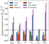 |
Fig. 4. Improvement factors of the several studied statistics over the redshift-space matter monopole+quadrupole constraints for each of the six cosmological parameters at kmax = 0.5 h Mpc−1. The horizontal black line shows the unity improvement. We note that these statistics exclude the combination with the matter multipoles and only concern the several cosmic web environments and their combination (therefore excluding the last line of Table 2 for instance). |
We also checked that including the hexadecapole (ℓ = 4) in our analysis does not lead to any further improvement of the constraints over the ℓ = {0, 2} statistics, neither for the matter nor for the environment-dependant spectra, or their combination.
5. Discussion and conclusion
It is well known that by analysing the matter distribution in redshift space through its power spectrum, we can greatly improve cosmological constraints. This is thanks to the velocity information contained in the anisotropy of the density fields, which breaks key degeneracies between parameters. Our results show that we can attain even tighter constraints by performing statistical analyses in identified cosmic web environments. In this configuration, the constraints on cosmological parameters, such as the initial spectral index, the matter density, the Hubble parameter, and most notably the summed neutrino mass, can be improved by up to a factor of two. Improvement factors can even reach five when combining these analyses with full matter statistics. Our approach therefore opens up a new avenue for the derivation of cosmological constraints via the analysis of the observed distribution of tracers. In particular, it shows that conditioning the correlations on the cosmic web environments improves constraints on the cosmological parameters compared to the direct correlation of all tracers, in agreement with previous findings (e.g. Uhlemann et al. 2020; Paillas et al. 2021, 2023).
The present study was performed in a theoretical context in which we built matter density fields from numerical simulations. Firstly, within this idealised context and with the studied statistics, it appears that constraining the cosmological parameters in redshift space yields similar constraints to those obtained in real space, if not tighter, despite the fact that we do not handle the distortions in the classification. This therefore suggests that reconstruction of the particles from redshift to real space (e.g. Jasche & Wandelt 2013; Bos et al. 2014; Leclercq et al. 2015) is not necessary in the present setting and can even deteriorate the accuracy of the derived constraints. Secondly, this context allows us to explore the full range of scales including non-linear ones. The combination of auto-spectra computed in the different environments up to kmax = 0.5 h Mpc−1 leads to tighter constraints in redshift than real space for most parameters, which is even more emphasised when adding information from the full matter monopole and quadrupole.
With this second paper of the series, we therefore go beyond showing how to use the cosmic web environments as leverage in order to improve the cosmological constraints in real space, and present the benefits of using a cosmic web classification to improve redshift-space constraints over the traditional matter power-spectrum multipoles. In a third paper, we will complete our comprehensive analysis of the cosmological content of the cosmic web environments with the analysis of the direct higher order statistic, namely the bispectrum. The next steps and challenges will consist in adapting and optimising our analysis – which is currently performed in a theoretical and idealised setup of large number density provided by particles in simulations – to more realistic cases of observed sparse tracers of the density field, such as halos or galaxies, as performed in other works (such as Hahn et al. 2020; Naidoo et al. 2022; Kreisch et al. 2022; Paillas et al. 2023). In this context, simulations will represent a major endeavour. Adapting our analysis so that it can be applied to actual data from galaxy surveys requires the exploitation of simulations with a higher mass resolution, enabling the definition of galaxy-type halos and with realistic baryonic physics models Vogelsberger et al. (2014). Such simulations will also allow us to bypass the difficulty of a theoretical modelling of covariance matrices and the building of likelihoods, which can be achieved with the use of simulation-based inference (e.g., Cranmer et al. 2020; Lemos et al. 2023). The information that can be gained on the cosmological content of cosmic web environments, as demonstrated by the results of the present study, will certainly justify the effort involved. The work presented here therefore constitutes a step towards an optimal and interpretable summary statistics that will allow us to take full advantage of the future Stage IV experiments (Laureijs et al. 2011; Spergel et al. 2015; DESI Collaboration 2016).
As all the particles have the same mass in the simulation, the ratio between Nα, the number of particles in the environment α, and the total number of particles N gives the mass fraction.
Acknowledgments
The authors thank the anonymous referee for their comments and further thank the members of the ByoPiC team (https://byopic.eu/team) for useful discussions. They also thank the Quijote team for making their data publicly available and particularly F. Villaescusa-Navarro for his help and availability regarding the Quijote suite. This research was supported by funding for the ByoPiC project from the European Research Council (ERC) under the European Union’s Horizon 2020 research and innovation program grant number ERC-2015-AdG 695561. A.D. was supported by the Comunidad de Madrid and the Complutense University of Madrid (Spain) through the Atracción de Talento program (Ref. 2019-T1/TIC-13298). T.B. acknowledges funding from the French government under management of Agence Nationale de la Recherche as part of the “Investissements d’avenir” program, reference ANR-19-P3IA-0001 (PRAIRIE 3IA Institute).
References
- Abbott, T. M. C., Allam, S., Andersen, P., et al. 2019, ApJ, 872, L30 [Google Scholar]
- Alam, S., Ata, M., Bailey, S., et al. 2017a, MNRAS, 470, 2617 [Google Scholar]
- Alam, S., Miyatake, H., More, S., Ho, S., & Mandelbaum, R. 2017b, MNRAS, 465, 4853 [CrossRef] [Google Scholar]
- Alam, S., Arnold, C., Aviles, A., et al. 2021, JCAP, 2021, 050 [Google Scholar]
- Allys, E., Marchand, T., Cardoso, J. F., et al. 2020, Phys. Rev. D, 102, 103506 [Google Scholar]
- Aragon-Calvo, M., Weygaert, R. V. D., & Jones, B. J. T. 2010, MNRAS, 408, 2163 [CrossRef] [Google Scholar]
- Bayer, A. E., Villaescusa-Navarro, F., Massara, E., et al. 2021, ApJ, 919, 24 [NASA ADS] [CrossRef] [Google Scholar]
- Bayer, A. E., Banerjee, A., & Seljak, U. 2022, Phys. Rev. D, 105, 123510 [NASA ADS] [CrossRef] [Google Scholar]
- Blake, C., Amon, A., Asgari, M., et al. 2020, A&A, 642, 1 [Google Scholar]
- Blot, L., Corasaniti, P. S., Alimi, J. M., Reverdy, V., & Rasera, Y. 2015, MNRAS, 446, 1756 [NASA ADS] [CrossRef] [Google Scholar]
- Bonnaire, T., Aghanim, N., Decelle, A., & Douspis, M. 2020, A&A, 637, A18 [NASA ADS] [CrossRef] [EDP Sciences] [Google Scholar]
- Bonnaire, T., Aghanim, N., Kuruvilla, J., & Decelle, A. 2021, A&A, 661, A146 [Google Scholar]
- Bonnaire, T., Decelle, A., & Aghanim, N. 2022, IEEE Trans. Pattern Anal. Mach. Intell., 44, 9119 [CrossRef] [Google Scholar]
- Bos, E. G., Van De Weygaert, R., Kitaura, F., & Cautun, M. 2014, Proc. Int. Astron. Union, 11, 271 [Google Scholar]
- Carron, J. 2013, A&A, 551, 10 [Google Scholar]
- Cautun, M., van de Weygaert, R., & Jones, B. J. 2013, MNRAS, 429, 1286 [NASA ADS] [CrossRef] [Google Scholar]
- Cautun, M., Weygaert, R. V. D., Jones, B. J. T., & Frenk, C. S. 2014, MNRAS, 441, 2923 [CrossRef] [Google Scholar]
- Chan, K. C., & Blot, L. 2017, Phys. Rev. D, 96, 023528 [NASA ADS] [CrossRef] [Google Scholar]
- Cheng, S., & Ménard, B. 2021, MNRAS, 8, 1 [Google Scholar]
- Cheng, S., Ting, Y.-S., Ménard, B., & Bruna, J. 2020, MNRAS, 499, 5902 [Google Scholar]
- Colas, T., D’Amico, G., Senatore, L., Zhang, P., & Beutler, F. 2020, JCAP, 06, 001 [NASA ADS] [Google Scholar]
- Cranmer, K., Brehmer, J., & Louppe, G. 2020, Proc. Natl. Acad. Sci., 117, 30055 [Google Scholar]
- D’Amico, G., Gleyzes, J., Kokron, N., et al. 2020, JCAP, 05, 005 [Google Scholar]
- DESI Collaboration (Aghamousa, A., et al.) 2016, ArXiv e-prints [arXiv:1611.00036] [Google Scholar]
- Drlica-Wagner, A., Mao, Y. Y., Adhikari, S., et al. 2019, ArXiv e-prints [arXiv:1902.01055] [Google Scholar]
- Eickenberg, M., Allys, E., Dizgah, A. M., et al. 2022, ArXiv e-prints [arXiv:2204.07646] [Google Scholar]
- Eisenstein, D. J., Zehavi, I., Hogg, D. W., et al. 2005, ApJ, 633, 560 [Google Scholar]
- Forero-Romero, J. E., Hoffman, Y., Gottlöber, S., Klypin, A., & Yepes, G. 2009, MNRAS, 396, 1815 [Google Scholar]
- Gualdi, D., Gil-marín, H., & Verde, L. 2021, JCAP, 2021, 008 [CrossRef] [Google Scholar]
- Hahn, C. H., & Villaescusa-Navarro, F. 2021, JCAP, 2021, 029 [CrossRef] [Google Scholar]
- Hahn, O., Porciani, C., Carollo, C. M., & Dekel, A. 2007, MNRAS, 375, 489 [NASA ADS] [CrossRef] [Google Scholar]
- Hahn, C. H., Villaescusa-Navarro, F., Castorina, E., & Scoccimarro, R. 2020, JCAP, 03, 040 [CrossRef] [Google Scholar]
- Hartlap, J., Simon, P., & Schneider, P. 2007, A&A, 464, 399 [NASA ADS] [CrossRef] [EDP Sciences] [Google Scholar]
- Hildebrandt, H., Viola, M., Heymans, C., et al. 2017, MNRAS, 465, 1454 [Google Scholar]
- Ivanov, M. M., Simonović, M., & Zaldarriaga, M. 2020, JCAP, 05, 042 [CrossRef] [Google Scholar]
- Jackson, J. 1972, MNRAS, 156, 74 [Google Scholar]
- Jasche, J., & Wandelt, B. D. 2013, MNRAS, 432, 894 [Google Scholar]
- Jullo, E., De La Torre, S., Cousinou, M. C., et al. 2019, A&A, 627, A137 [NASA ADS] [CrossRef] [EDP Sciences] [Google Scholar]
- Kaiser, N. 1987, MNRAS, 227, 1 [Google Scholar]
- Kaufman, G. 1967, Center for Operations Research and Econometrics, 44 [Google Scholar]
- Kodwani, D., Alonso, D., & Ferreira, P. G. 2019, Open J. Astrophys., 2, 3 [NASA ADS] [CrossRef] [Google Scholar]
- Kreisch, C. D., Pisani, A., Villaescusa-Navarro, F., et al. 2022, ApJ, 935, 100 [NASA ADS] [CrossRef] [Google Scholar]
- Kuruvilla, J. 2022, A&A, 660, A113 [NASA ADS] [CrossRef] [EDP Sciences] [Google Scholar]
- Kuruvilla, J., & Aghanim, N. 2021, A&A, 653, A130 [NASA ADS] [CrossRef] [EDP Sciences] [Google Scholar]
- Laureijs, R., Amiaux, J., Arduini, S., et al. 2011, ArXiv e-prints [arXiv:1110.3193] [Google Scholar]
- Leclercq, F., Jasche, J., Lavaux, G., & Wandelt, B. 2015, ArXiv e-prints [arXiv:1512.02242] [Google Scholar]
- Lemos, P., Cranmer, M., Abidi, M., et al. 2023, Mach. Learn.: Sci. Technol., 4, 01LT01 [NASA ADS] [CrossRef] [Google Scholar]
- Libeskind, N. I., van de Weygaert, R., Cautun, M., et al. 2017, MNRAS, 473, 1195 [Google Scholar]
- Mandelbaum, R., Slosar, A., Baldauf, T., et al. 2013, MNRAS, 432, 1544 [NASA ADS] [CrossRef] [Google Scholar]
- Martizzi, D., Vogelsberger, M., Artale, M. C., et al. 2019, MNRAS, 486, 3766 [Google Scholar]
- Massara, E., Villaescusa-Navarro, F., Ho, S., Dalal, N., & Spergel, D. N. 2021, Phys. Rev. Lett., 126, 1 [CrossRef] [Google Scholar]
- Massara, E., Villaescusa-Navarro, F., Hahn, C., et al. 2022, ArXiv e-prints [arXiv:2206.01709] [Google Scholar]
- Mueller, E. M., Bernardis, F. D., Bean, R., & Niemack, M. D. 2015, ApJ, 808, 47 [NASA ADS] [CrossRef] [Google Scholar]
- Naidoo, K., Whiteway, L., Massara, E., et al. 2020, MNRAS, 491, 1709 [NASA ADS] [CrossRef] [Google Scholar]
- Naidoo, K., Massara, E., Lahav, O., et al. 2022, MNRAS, 513, 3596 [NASA ADS] [CrossRef] [Google Scholar]
- Paillas, E., Cai, Y. C., Padilla, N., & Sánchez, A. G. 2021, MNRAS, 505, 5731 [NASA ADS] [CrossRef] [Google Scholar]
- Paillas, E., Cuesta-Lazaro, C., Zarrouk, P., et al. 2023, MNRAS, 522, 606 [CrossRef] [Google Scholar]
- Peacock, J. A., Cole, S., Norberg, P., et al. 2001, Nature, 410, 169 [Google Scholar]
- Philcox, O. H., & Ivanov, M. M. 2022, Phys. Rev. D, 105, 43517 [Google Scholar]
- Sousbie, T. 2011, MNRAS, 414, 350 [NASA ADS] [CrossRef] [Google Scholar]
- Spergel, D., Gehrels, N., Baltay, C., et al. 2015, Wide-Field InfrarRed Survey Telescope-Astrophysics Focused Telescope Assets WFIRST-AFTA 2015 Report, Tech. Rep. [Google Scholar]
- Stoica, R. S., Martínez, V. J., & Saar, E. 2007, J. R. Stat. Soc. Ser. C: Appl. Stat., 56, 459 [CrossRef] [Google Scholar]
- Takahashi, R., Yoshida, N., Takada, M., et al. 2010, ApJ, 726, 7 [Google Scholar]
- Tempel, E., Stoica, R. S., Martínez, V. J., et al. 2014, MNRAS, 438, 3465 [CrossRef] [Google Scholar]
- Totsuji, H., & Kihara, T. 1969, Astron. Soc. Jpn., 21, 221 [NASA ADS] [Google Scholar]
- Uhlemann, C., Friedrich, O., Villaescusa-Navarro, F., Banerjee, A., & Codis, S. 2020, MNRAS, 495, 4006 [NASA ADS] [CrossRef] [Google Scholar]
- Valogiannis, G., & Dvorkin, C. 2022a, Phys. Rev. D, 105, 103534 [Google Scholar]
- Valogiannis, G., & Dvorkin, C. 2022b, Phys. Rev. D, 106, 103509 [Google Scholar]
- Villaescusa-Navarro, F., Banerjee, A., Dalal, N., et al. 2018, ApJ, 861, 53 [NASA ADS] [CrossRef] [Google Scholar]
- Villaescusa-Navarro, F., Hahn, C., Massara, E., et al. 2020, ApJS, 250, 2 [CrossRef] [Google Scholar]
- Vogelsberger, M., Genel, S., Springel, V., et al. 2014, MNRAS, 444, 1518 [Google Scholar]
- Wang, Y., & He, P. 2022, ApJ, 934, 112 [Google Scholar]
- Wang, Y., Yang, H.-Y., & He, P. 2022, ApJ, 934, 77 [Google Scholar]
- Woodfinden, A., Nadathur, S., Percival, W. J., et al. 2022, MNRAS, 516, 4307 [NASA ADS] [CrossRef] [Google Scholar]
Appendix A: Fisher formalism
The Fisher formalism allows the forecast of constraints we will get on our set of parameters θ = {Ωm, Ωb, h, ns, σ8, Mν} based on a statistical summary of the density fields. In our case, this summary is given by the set of environment-dependent (cross- or auto-)power spectra in Fourier bins, s = {Pαβ(k)}. Assuming a Gaussian likelihood with a covariance matrix that is independent of cosmology (Carron 2013; Kodwani et al. 2019), we can derive elements of the Fisher information matrix as
![Mathematical equation: $$ \begin{aligned} \left[\boldsymbol{I}(\boldsymbol{\theta })\right]_{i,j} = \left(\frac{\partial \bar{\boldsymbol{s}}}{\partial \theta _i}\right)^\mathsf{T } \boldsymbol{\Sigma }^{-1} \left(\frac{\partial \bar{\boldsymbol{s}}}{\partial \theta _j}\right)\cdot \end{aligned} $$](/articles/aa/full_html/2023/06/aa45626-22/aa45626-22-eq36.gif) (A.1)
(A.1)
The first ingredient in the computation of the Fisher information matrix is the unbiased estimate of the inverse covariance matrix Σ−1, which is given, still under the Gaussian assumption, by (Kaufman 1967; Hartlap et al. 2007)
 (A.2)
(A.2)
where Nfid is the number simulations at the fiducial cosmology, n is the length of the summary statistics vector s, and  is the unbiased estimate of the covariance matrix.
The second ingredient of Eq. (A.1) are the derivatives with respect to the parameters of the model θ. These latter can be estimated numerically from the Nderiv = 500 realisations of the variation of individual parameters in the Quijote suite as
 (A.3)
(A.3)
However, we note that the above definition does not apply for Mν being a positive quantity with a fiducial value at 0.0 eV. For this parameter, we therefore rely on the four-point forward approximation of the derivative
 (A.4)
(A.4)
where  = 0.1 eV. For consistency, we use a set of simulations initialised using the Zel’dovich approximation to compute
  in the previous equation because all the other terms are initialised this way. The presented results are obtained by making use of Nderiv = 500 and Nfid = 7000 realisations to respectively compute the derivatives and the covariance matrix.
Appendix B: Covariance matrices, derivatives, and confidence ellipses
While discussed in the main text Sect. 4, we report in this section the two ingredients of the Fisher quantification of information, which are: (i) the correlation matrices between the several elements of the statistic vector in Fig. B.1 and (ii) the derivatives of the redshift-space monopoles and quadrupoles with respect to the six cosmological parameters. Figure B.2 shows the corner plot with the several confidence ellipses obtained for the  statistics for all six cosmological parameters, namely Ωm, Ωb, h, ns, σ8, and Mν.
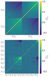 |
Fig. B.1. Correlation coefficients Cij obtained from Nfid = 7000 simulations for (top) the matter power spectrum, and (bottom) from the auto-spectra Pαα(k) computed in the different environments. Each submatrix goes from k = 0.1 h/Mpc to k = 0.5 h/Mpc. |
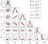 |
Fig. B.2. 1σ confidence ellipses for all the pairs of cosmological parameters (Ωm,Ωb,h,ns,σ8,Mν) obtained from the several statistics (either the matter monopole+quadrupole or the ones from the environments and their combination) in redshift space. The normalised probability density functions for each parameter are shown on the diagonal. |
Appendix C: Constraints from spectra in the several environments
Here, we provide the individual constraints obtained from the monopole and quadrupole power spectra computed in the different cosmic web environments in Table C.1. As discussed in Sect. 4, they all lead to much weaker constraints than the full matter statistic in redshift-space when kmax = 0.5 h/Mpc. However, their combination leads to tighter constraints with an improvement by a factor of up to 2.7 for the summed neutrino mass and 2.4 for ns.
Marginalised 1σ constraints obtained from the analysis of power-spectra monopoles and quadrupoles computed in the different environments for all cosmological parameters.
All Tables
Averaged confusion matrix obtained from ten boxes of the Quijote simulations with the fiducial cosmology when considering the absence of RSD as a ground truth.
Marginalised 1σ constraints obtained from the analysis of power-spectra monopoles and quadrupoles computed in the different environments for all cosmological parameters.
Marginalised 1σ constraints obtained from the analysis of power-spectra monopoles and quadrupoles computed in the different environments for all cosmological parameters.
All Figures
|
Fig. 1. Ratio between the redshift-space and real-space monopoles computed in the cosmic web environments. The grey shaded region shows the scales k > 0.5 h Mpc−1, which are unused in this analysis. |
| In the text | |
|
Fig. 2. Residuals of the matter monopole (upper left panel) or quadrupole (upper right panel) and environment-dependent monopoles (lower left panel) or quadrupoles (lower right panel) when varying either σ8, Ωm, or Mν. Residuals are defined as |
| In the text | |
|
Fig. 3. Evolution of the marginalised constraint σθi given by |
| In the text | |
|
Fig. 4. Improvement factors of the several studied statistics over the redshift-space matter monopole+quadrupole constraints for each of the six cosmological parameters at kmax = 0.5 h Mpc−1. The horizontal black line shows the unity improvement. We note that these statistics exclude the combination with the matter multipoles and only concern the several cosmic web environments and their combination (therefore excluding the last line of Table 2 for instance). |
| In the text | |
|
Fig. B.1. Correlation coefficients Cij obtained from Nfid = 7000 simulations for (top) the matter power spectrum, and (bottom) from the auto-spectra Pαα(k) computed in the different environments. Each submatrix goes from k = 0.1 h/Mpc to k = 0.5 h/Mpc. |
| In the text | |
|
Fig. B.2. 1σ confidence ellipses for all the pairs of cosmological parameters (Ωm,Ωb,h,ns,σ8,Mν) obtained from the several statistics (either the matter monopole+quadrupole or the ones from the environments and their combination) in redshift space. The normalised probability density functions for each parameter are shown on the diagonal. |
| In the text | |
Current usage metrics show cumulative count of Article Views (full-text article views including HTML views, PDF and ePub downloads, according to the available data) and Abstracts Views on Vision4Press platform.
Data correspond to usage on the plateform after 2015. The current usage metrics is available 48-96 hours after online publication and is updated daily on week days.
Initial download of the metrics may take a while.