| Issue |
A&A
Volume 696, April 2025
|
|
|---|---|---|
| Article Number | A168 | |
| Number of page(s) | 12 | |
| Section | Galactic structure, stellar clusters and populations | |
| DOI | https://doi.org/10.1051/0004-6361/202453187 | |
| Published online | 21 April 2025 | |
Kinematics of metallicity populations in Omega Centauri using the Gaia Focused Product Release and Hubble Space Telescope
1
Dipartimento di Fisica e Astronomia, Università di Padova,
vicolo dell’Osservatorio 2,
35122
Padova,
Italy
2
INAF – Ossevatorio Astronomico di Padova,
vicolo dell’Osservatorio 5,
35122
Padova,
Italy
3
National Astronomical Observatory of Japan,
2-21-1 Osawa, Mitaka,
Tokyo
181-8588,
Japan
4
Institute for Astronomy, University of Edinburgh, Royal Observatory,
Blackford Hill,
Edinburgh
EH9 3HJ,
UK
★ Corresponding author; This email address is being protected from spambots. You need JavaScript enabled to view it.
; This email address is being protected from spambots. You need JavaScript enabled to view it.
Received:
27
November
2024
Accepted:
24
February
2025
Abstract
Context. Omega Cen is the largest known globular cluster in the Milky Way. It is also a quite complex object with a large metallicity spread and multiple stellar populations. Despite a number of studies over the past several decades, the series of events that led to the formation of this cluster is still poorly understood. One of its peculiarities is the presence of a metal-rich population that does not show the phenomenon of light-element anti-correlations (C-N, Na-O, Mg-Al), a trait that is considered characteristic of Galactic globular clusters and present among more metal-poor Omega Cen stars. This leads to speculation that such an anomalous population was accreted by the cluster.
Aims. We aim to investigate the kinematics of Omega Cen populations to gain insight into the formation scenario of the cluster.
Methods. Using the newly released Gaia FPR and DR3 catalogue, we conducted a detailed kinematical analysis of cluster members within Omega Cen. The cluster members were divided into four metallicity populations, and their mean proper motion in radial and tangential components were compared with each other. We also performed Gaussian-mixture model fitting on the metallicity distribution to estimate the number of populations within our sample and an independent analysis of the Hubble Space Telescope catalogue as confirmation.
Results. The mean proper motions (μr and μt) of the metallicity populations do not show any significant differences. It is also not dependent on the approach chosen to determine the number of metallicity populations. We do find a clear signature of rotation in all of the populations (including the metal-rich one) with similar velocities.
Key words: astrometry / proper motions / globular clusters: general
© The Authors 2025
 Open Access article, published by EDP Sciences, under the terms of the Creative Commons Attribution License (https://creativecommons.org/licenses/by/4.0), which permits unrestricted use, distribution, and reproduction in any medium, provided the original work is properly cited.
This article is published in open access under the Subscribe to Open model. This email address is being protected from spambots. You need JavaScript enabled to view it. to support open access publication.
1 Introduction
During a galactic merger, the larger galaxy usually disrupts the dwarf galaxy through tidal interactions (Helmi & White 2001; Mayer et al. 2002), and a large percentage of the stars from the dwarf galaxy are dispersed into the halo of the larger galaxy (in our case, the larger galaxy being the Milky Way). Even with these strong disruption events, the dense central nuclear star clusters (NSCs) of the dwarf galaxies (Neumayer et al. 2020) can survive and live within the halo of the host galaxy (one example is given in Pfeffer & Baumgardt 2013). After stripping the external galactic components, the NSC will look similar to a large globular cluster (GC; Georgiev & Böker 2014; Neumayer et al. 2020) as they have a similar mass and radius. The Milky Way has undergone a series of mergers, the last major one being the Gaia-Enceladus satellite merger about 10 Gyr ago (Haywood et al. 2018; Helmi et al. 2018). It is also currently undergoing a merger with the Sagittarius dwarf galaxy (Ibata et al. 1997; Laporte et al. 2018). Pfeffer et al. (2014); Kruijssen et al. (2019) looked at models of galactic formation and predicted that about six (±1) clusters in the halo of the Milky Way were likely to be NSCs of other galaxies that were ingested. One example that has been identified as one such stripped NSC is M54, the remnant of the Sagittarius dwarf spheroidal galaxy, with the stripped stars forming a stream that wraps around the Milky Way (Alfaro-Cuello et al. 2019, 2020; Kacharov et al. 2022).
Omega Centauri (Omega Cen) is quite a unique object in the Milky Way, not only because it is the most massive GC in the Galaxy, but also due to the complexity of the stellar populations within it. Omega Cen, just like any other GC, was thought to be a simple ensemble of stars formed from the same molecular cloud, with identical ages and formed with the same chemical composition. But in the early 1970s, the evidence of metallicity spread was reported by Freeman & Rodgers (1975). By the late 1990s, it was also reported to host multiple stellar populations Anderson (1997); Lee et al. (1999); Pancino et al. (2000); Bedin et al. (2004), and more extensive colour-magnitude diagram (CMD) work using the HST1 data by Bellini et al. (2017a) revealed the presence of multiple stellar populations at all the evolutionary stages. Due to these characteristics, Omega Cen has been suggested as the former nucleus of a dwarf galaxy which was ingested by the Milky Way. Evidence in support of this hypothesis has been put forward in recent years, from the presence of an internal stellar disc (van de Ven et al. 2006) to a possible association with the Gaia-Enceladus orbit (Massari et al. 2019; Pfeffer et al. 2021; Callingham et al. 2022; Limberg et al. 2022), the presence of a counter-rotating population (Pechetti et al. 2024), and an intermediate black hole in the centre of the cluster (Häberle et al. 2024b).
High- and intermediate-resolution spectroscopy have been extensively used to characterise the composition of the stellar populations within Omega Cen (Norris et al. 1996; Sollima et al. 2005a; Villanova et al. 2007; Johnson & Pilachowski 2010; Villanova et al. 2014; Alvarez Garay et al. 2024; Nitschai et al. 2024). These studies have found the metal-poor and metal-intermediate populations show anti-correlation in Na-O and Mg-Al abundances, a behaviour consistent with what is observed in all Galactic GCs. However, the metal-rich population, at [Fe/H] ∼ −0.9 dex, does not show such anti-correlations, but instead shares the behaviour of Na, O, Mg, and Al, with field stars. This is not only an abnormal behaviour for GC stars, but also completely different from that of the dominant population of Omega Cen. Due to this, metal-rich has usually been referred to as the anomalous population.
The origin of the anomalous population is still being debated, with at least three scenarios being put forward. The first scenario is the ingestion of the field stars of the dwarf galaxy into the central NSC during the disruption event of the merger. This scenario has been linked to the formation mechanism of M54 (Carretta et al. 2010), which is analogous to Omega Cen. The second scenario is the merger of two clusters (one large metal-poor cluster and another one relatively smaller and metal-rich), and the third scenario is that of self-enrichment by the first generation asymptotic giant branch (AGB) stars and Type-II supernovae (Norris et al. 1996; Smith et al. 2000). Except for the self-enrichment, the other two scenarios require the metal-rich population to be brought into the cluster and therefore, in those cases, the kinematics of the metal-rich stars could still bear the signature of their different origin. In fact, given Omega Cen’s long relaxation time (about ∼ 109 yr in the centre and ∼ 1010 yr at half-light radius Meylan et al. 1995; van de Ven et al. 2006), such a signature would be detectable long after the ingestion of the anomalous population, especially when probing the outskirts of the cluster.
Previously, Ferraro et al. (2002) used photometry from Pancino et al. (2000) and proper motions from van Leeuwen et al. (2000) to investigate the proper motions of the four metallicity populations and concluded that the mean motion of the metal-rich population was not consistent with the other populations and therefore, it might have been the accreted one. However, the result was contested by Platais et al. (2003), who claimed the difference in proper motions reported by van Leeuwen et al. (2000) was caused by instrumental effects, whereas Hughes et al. (2004) argued the results were valid because van Leeuwen et al. (2000) had made necessary correction. Later, Bellini et al. (2009) used ground-based data and Bellini et al. (2018); Libralato et al. (2018) both used HST data and found no significant difference in the motions of the populations. Even though HST data were considerably more precise than the ground-based data, they only covered a small region in the exterior of the cluster. Sanna et al. (2020) conduced the same analysis of the motions, but using the Gaia DR2 data for the RGB stars, and again found no significant differences. The availability of Gaia DR3 and FPR data combined with the recent publication of the MUSE based oMEGACat catalogues (Nitschai et al. 2023; Häberle et al. 2024a) allows us to revisit the issue.
In this study, we used photometry and metallicities from Nitschai et al. (2023) and astrometry from Gaia to look at the motions of populations. This gives three advantages compared to the analyses conducted in previous studies: 1. complete coverage of Omega Cen, from the outer regions to the dense central core region (see Section 2.1); 2. a larger sample compared to previous studies; and 3. inclusion of fainter main-sequence stars (up to 2 mag fainter than the turn-of star). These advantages allowed us to obtain better constraints on the motions of the populations than ever before. In Section 2, we describe the datasets used for the analysis along with their respective selection criteria, quality cuts, and methods of cross-matching different catalogues. In Section 3, we provide the procedures for selecting metallicity populations and converting proper motions from Gaia to radial and tangential components, and we include confirmation of the results using another dataset from the HST. The interpretation of all the results is given in Section 4, with concluding remarks provided in Section 5.
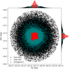 |
Fig. 1 Distribution of stars observed by Gaia DR3 and Gaia FPR and oMEGACat II catalogue from Häberle et al. (2024a). Gaia FPR data are relatively more complete in the central region of Omega Cen in comparison to DR3, whereas oMEGACat II is complete in the very centre of the cluster. |
2 Data
2.1 Datasets
In order to study the astrometry of stars within Omega Cen, we used the newly released Gaia Focused Product Release (FPR; Gaia Collaboration 2023c) catalogue in addition to Gaia DR3 (Gaia Collaboration 2023b). Gaia FPR was released on 10 October 2023, and in most cases it builds on the DR3 catalogue by providing astrometry and photometry for many additional sources.
In the data released so far by Gaia, there is a limited coverage within dense fields. This is due to the astrometric crowding limitations of the readout window strategy, which is generally used during Gaia's nominal mission. This method works well up to an object density of 1 050 000 deg2 (Gaia Collaboration 2023c), but the density in central regions of GCs such as Omega Cen is significantly higher than this limit. The incompleteness of Gaia DR3 is shown in Fig. 1. To address this incompleteness issue within the catalogues, the Gaia Data Processing and Analysis Consortium (DPAC) applied a new software pipeline for the FPR catalogue, where two-dimensional service interface function (SIF) images are used to obtain information about nearby sources and accurately measure the astrometry of faint and crowded stars (Gaia Collaboration 2023c). Gaia FPR has a total of 526 587 objects for the Omega Cen region; while using a cone search with a radius of 1 deg for Omega Cen within Gaia DR3, we obtained about 400 000 stars.
The following step was to filter out the non-cluster members from the sample. For the DR3 objects, we adopted the membership probabilities from Vasiliev & Baumgardt (2021) (which is based on Gaia EDR3) and set a threshold membership probability of 95% or higher for the analysis. As all the FPR stars are new sources with no overlap with the previous Gaia catalogues, there are no membership probabilities for them in the literature. Thus, we defined a spatial region using the DBSCAN clustering algorithm (Ester et al. 1996) and convex hull that encompassed the DR3 bona fide members as shown in Fig. 2 and then considered any star from the FPR catalogue falling within this defined region as a cluster member. In addition to this, we also defined bounds in the proper motions of the stars, where we included stars with proper motions in RA and Dec to be within ±5 mas of the cluster’s mean proper motions in RA and Dec (taken from Baumgardt et al. 2019), respectively. The necessity for this selection criterion is due to the presence of stars with highly discrepant proper motions compared to the known motion of the cluster, as seen in Fig. 3. Even though the mentioned method may not seem robust enough, given the high density of cluster members in the interior of the cluster, the percentage of background or foreground stars making it into the final sample should be minimal and may not have a significant effect on the analysis. More importantly, by relying on the spacial selection criteria and not just on the proper motions, we ensured our final sample was free of any biases, whereby one of the populations that has a different mean proper motion compared to the dominant population of the cluster could be mislabelled as discrepant and not belonging to the cluster. As for the potential bias caused by the spatial distribution of populations – where centrally concentrated stars from one population are included while those from another population more prevalent in the outskirts are excluded – this is not a concern. Nitschai et al. (2024) showed that the cluster is well mixed within the half-light radius, thus eliminating any spatial bias. Consequently, our final sample comprises 520 000 stars, with 370 000 from FPR and 150 000 from DR3.
Along with the Gaia catalogue, we also analysed the oMEGACat II catalogue (Häberle et al. 2024a), which provides precise HST astrometry for about 1.5 million stars in the inner region of Omega Cen. Compared to Gaia FPR, oMEGACat II not only provides precise astrometry for significantly more centrally located stars (as seen in Fig. 1), it also includes relatively fainter main-sequence stars (up to 26 mag in F435W filter).
The metallicities and radial velocities (RVs) of the stars were obtained from the oMEGACat I catalogue (Nitschai et al. 2023). They used spectroscopic data from MUSE to measure the metallicities and RV of more than 300 000 stars within the half-light radius of Omega Cen. In addition to this, the catalogue provides the brightness of the objects in two HST Advanced Camera for Surveys (ACS) filters (F435W and F625W).
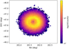 |
Fig. 2 Distribution of Gaia EDR3 stars from Vasiliev & Baumgardt (2021) with membership probability ≥95%. The colour represents the number of stars within each hexbin. The black circle is the spacial region used to filter Gaia FPR stars. |
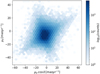 |
Fig. 3 Distribution of proper motions in RA and Dec of all the Gaia FPR stars. Many stars have significantly larger proper motions than the mean proper motion of the cluster. The colour represents the number of stars within each hexbin. |
2.2 Cross-matching
oMEGACat I is a catalogue based on HST photometry, and it does not include Gaia IDs for the targets. Given that the cluster is a very dense environment, simple position cross-matching between oMEGACAt I and Gaia DR3 and FPR might potentially lead to misidentifications. To minimise these events, we also filtered by the stellar magnitude. As there are no common filters between the photometric systems, we derived transformation equations between the G magnitude and F435W and F625W passbands.
For this, the Gaia BP/RP (XP) continuous spectra for about 3000 stars from three clusters (M67, NGC 188 and M15) were used. These clusters were chosen in order to cover a wide metallicity range (M67:[Fe/H] ≃ 0.0 dex, NGC 188:[Fe/H] ≃ 0.1 dex and M15: [Fe/H] ≃ −2.3 dex) and to include a large number of stars in the evolutionary phases. These XP spectra were input into the Generator routine of the GaiaXPy package to calculate the synthetic HST photometry, including the F435W and F625W band magnitudes. With the two pseudo magnitudes, a simple polynomial curve fitting using the equation y = Ax3 + Bx2 + Cx + D provides the transformation equation, where y is (G – F435W) and x is (F625W – F435W), and the values of the coefficients are given in Table 1. While there is no expectation that this simple approach leads to a highly accurate transformation such as that in Gaia Collaboration (2023a), it serves the purpose of improving the accuracy of the cross-matching in a dense field.
The cross-matching was performed by adopting a search radius of 0.5′′ and a magnitude difference of less than 1 mag between the Gaia G-band magnitude and pseudo G-band magnitude of the oMEGACat I catalogue. The low value of the search radius is due to the high density of stars in the region, and a 1 mag photometric threshold was used by taking into account the uncertainties involved in the conversion of HST photometry into pseudo G-band magnitude. With the above criteria, 224 361 of the 520 000 objects had a match. We note that the number of matches is not sensitive to the selection criteria used. By doubling the search radius to 1′′, we only obtain about 13 000 (about 6%) additional matches, and by increasing the photometric threshold to 1.5 mag, we obtain 18 000 (about 9%) additional matches. This low sensitivity to selection criteria is due the inclusion of both coordinate and photometric searches. A colour-magnitude diagram (CMD) of all the cross-matched stars is shown in the left panel of Fig. 4.
Values of coefficients obtained by performing polynomial curve fitting.
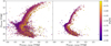 |
Fig. 4 Left: CMD of all stars within our Gaia sample that match with the oMEGACat I catalogue. Right: CMD of stars that are included in the high-quality sample. |
2.3 Quality cuts
As the aim is to be able to detect even subtle differences in the motions of different populations, it is important to only retain accurate measurements for the analysis. The usual Gaia selection filters were applied, where we only included stars with astrometric excess noise with a value below two and renormalised the unit weight error between 0.8 and 1.2. We also refined the sample using the quality flags detailed in Nitschai et al. (2023). These quality cuts brought down our sample significantly, from 224 361 cross-matched stars to 28 607 stars. This is a nearly 90% decrease in the sample size and due to the large astrometric excess noise in majority of the centrally located Gaia FPR stars. These stars most likely suffered from intense crowding, which led to large excess noise. The selected stars (referred to as the high-quality sample) are plotted on the CMD in the right panel of Fig. 4.
3 Analysis
3.1 Metallicity populations
Literature studies have adopted spectroscopic or photometric approaches to identify various populations in Omega Cen. Interestingly, though, different studies, even when using similar approaches, have reported the existence of varying numbers of metallicity populations within the cluster. For example, an early study by Hesser et al. (1985) reported bimodality in the metallicity distribution in Omega Cen, which was later confirmed by Norris et al. (1996) using calcium abundances and by Anderson (1997) and Bedin et al. (2004) using HST photometry. In the early 2000s, studies such as Sollima et al. (2005b) and Villanova et al. (2007, 2014) looked at the sub-giant branch (SGB) of Omega Cen using spectroscopy and reported the existence of four, four, and six populations, respectively. Johnson & Pilachowski (2010) conduced a spectroscopic study on the red-giant branch (RGB) of Omega Cen and reported five populations, while Pancino et al. (2000) used photometry and reported three populations. Sollima et al. (2005a) and Calamida et al. (2009) used FORS1 and Stromgren photometry, respectively, on the RGB to find five and four populations, respectively. In recent times, Bellini et al. (2017b) used HST photometry and chromosome maps to photometrically identify at least 15 populations, out of which nine have been confirmed by Husser et al. (2020). Recently, two studies Alvarez Garay et al. (2024) hereafter AG24; and Nitschai et al. (2024) hereafter SN24; looked at the metallicity populations using spectroscopy. AG24 used high-resolution spectroscopic data from VLT/FLAMES to study the Mg-Al anti-correlation with a sample of 439 RGB stars within Omega Cen. They clearly find four populations in their metallicity distribution (see Fig. 2 of their paper) with peaks at −1.85, −1.55, −1.15, and −0.80 dex. Conversely, SN24 used metallicities taken from the oMEGACat I catalogue (Nitschai et al. 2023), which is based low-resolution MUSE data, to study a sample of 11 050 RGB stars, finding 11 different populations.
Given such a diversity of populations being reported, we used two different methods to divide our sample. The first method is to use the bounds defined in existing literature, while the second method is to estimate the number of populations directly within our sample.
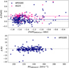 |
Fig. 5 Top: comparison between metallicities of oMEGACat I catalogue with that from AG24 (pink cross) and APOGEE (purple circles). The purple and pink dashed line represents the mean offset of AG24 and APOGEE from oMEGACat I metallicities, respectively. Bottom: comparison of radial velocities between oMEGACat I and APOGEE. The y-axes of the top and bottom panels represent [Fe/H]oMEGACatI − [Fe/H]lit and RVoMEGACatI − RVlit, respectively. |
3.1.1 Method 1: literature
For this analysis, we used the metallicity bounds defined by AG24, the most recent high-resolution study of the chemistry of stars within the cluster. We selected this study over SN24, despite it being the latest research on Omega Cen populations and having the largest sample to date, because SN24’s analysis is based on metallicities derived from low-resolution spectroscopic data, resulting in larger measurement uncertainties. In contrast, AG24 utilised spectroscopic data with a resolution of 20 000–29 500 and a signal-to-noise ratio of 70–100. This higher resolution and quality enabled AG24 to better constrain the metallicities of even the most metal-poor stars ([Fe/H] < −2.0 dex), providing more reliable metallicity bounds for the populations.
Before dividing our sample into sub-populations following AG24, we probed the existence of any offsets or trends in the metallicities from oMEGACat I (used for the analysis) with respect to AG24 (used to define bounds). In the top panel of Fig. 5, we compare oMEGACat I metallicities with AG24 and APOGEE2 (Jönsson et al. 2020). We find a mean metallicity difference between AG24 and oMEGACat I to be about 0.2 dex. Therefore, to account for this offset within the analysis, we adopted a correction factor of 0.2 dex on the oMEGACat I metallicities. With respect to APOGEE, the mean metallicity difference is smaller at 0.07 dex. In the bottom panel, we also compare the RVs from oMEGACat I and APOGEE, where we find a good agreement between the two.
Following AG24, we divide our sample into four subpopulations defined as metal-rich (MR, [Fe/H] ≥ −0.93 dex), metal-intermediate a (MIa, −1.33 ≤ [Fe/H] < −0.93 dex), metal-intermediate b (MIb, −1.68 ≤ [Fe/H]<−1.33 dex), and metal-poor (MP, [Fe/H] < −1.68 dex). The metallicity distribution of the four populations and their corresponding locations in the CMD are shown in Fig. 6 (left and right panels, respectively). The metallicity distribution and the four sub-populations are shown in the left panel of Fig. 6, with the CMD of the four sub-populations in the right panel of Fig. 6.
From Fig. 6, it can be noticed that the metallicity distribution of our sample is quite different from the one in AG24. This could be due to several factors, such as larger uncertainties on the metallicities in the oMEGACat I catalogue, different sample size, or different stellar types (our sample includes RGB and turn-off stars, as well as main sequence stars that are up to 3 mag fainter than turn-off stars in the F625W filter band, whereas AG24 only includes RGB stars).
In Fig. 7, the top panel shows the individual CMDs of the populations. All of the populations have a well-defined main sequence, but only the metal-intermediate-b and metal-poor populations have well-populated RGBs, with metal-intermediate-a and metal-rich populations having only a few stars. The bottom panel shows the mean metallicity of different magnitude bins within each population. In three populations (i.e. MR, MIa and MIb), the maximum differences between metallicities corresponding to the MS and RGB are about 0.04, 0.05, and 0.03 dex, respectively. However, in the MP population this difference is about 0.18 dex (with the RGB being more metal rich), with it increasing to 0.24 dex between turn-off and RGB stars. This offset could be attributed to the difficulty of parameter estimation at such low metallicities using a low-resolution spectrum.
3.1.2 Method 2: metallicity-distribution fitting
An alternative approach is to estimate the number of subpopulations within our sample by fitting the metallicity distribution using the Gaussian mixture model (GMM) provided under the Scikit-learn3 Python package (Pedregosa et al. 2011). We fitted the metallicity distribution with GMMs consisting of different numbers of components (ranging from 2 to 20). The best-fit model was selected using the Bayesian information criterion (BIC), which in our case is six components. The fitting of the metallicity distribution and individual components of the best fit is shown in Fig. 8, with the results of the fitting in Table 2. The six peaks are at [Fe/H] −2.35, −1.95, −1.60, −1.25, −1.05, and −0.60 dex. For comparison, the four peaks found in AG24 are at −1.85, −1.55, −1.15, and −0.80 dex. Three of the six peaks in this study, that is, −1.95, −1.60, and −1.25 dex, are within 1σ of the first three peaks of AG24, with our values being larger. The peak at −1.05 dex is slightly more discrepant compared to −0.80 dex of AG24 but is within the 3σ range. Along with these four, we also find one most metal-poor peak and another most metal-rich peak at −2.35 and −0.60 dex, respectively. The most metal-poor peak is consistent (within 1σ) with the metal-poor population found in Johnson et al. (2020) at −2.25 dex. However, this peak in Johnson et al. (2020) only contained 11 stars, whereas in this case it amounts to over 900 stars. However, the two sub-populations at −2.35 and −0.60 dex constitute less than 6% of the total sample, with 68% of the stars having an [Fe/H] between −1.78 and −1.03 dex.
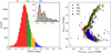 |
Fig. 6 Left: metallicity distribution of our sample with the one from AG24 shown in the inserted panel. Different metallicity populations are represented by different colours. Right: CMD of different sub-populations. |
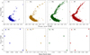 |
Fig. 7 Top: individual CMDs of populations from metal-rich ones in the leftmost panel to metal-poor ones in the rightmost panel. Bottom: mean metallicities of magnitude bins within different populations. |
3.2 Proper motion
We used the Gaia proper motions ( 4 and μδ) to analyse the motions of the sub-populations. Given the high sensitivity needed to decipher small differences among the populations, we investigated the precision of the Gaia measurements, specifically the proper motions’ components. In Fig. 9, we plot
  and μδ in the upper panels with their corresponding errors in the lower panels. Based on Gaia DR2 data, the mean proper-motion values for Omega Cen are
  and μδ = −6.73 mas yr−1 (Baumgardt et al. 2019) and are represented with a dashed black line in Fig. 9. It is evident from Fig. 9 that the proper-motion measurements are more likely to deviate from the average value as we go towards fainter stars. This is an expected behaviour as it is difficult to accurately identify and accurately measure the position of faint stars in a dense field. In addition to this deviation, we also see the uncertainties on the measurements rapidly increase as we approach fainter magnitudes. This effect is exaggerated in Gaia FPR compared to DR3, as the former mostly provides data for objects close to the core of the cluster. To remove any adverse effects of these large uncertainties from our analysis, we decided to use only the best 20% of the measurements in each magnitude bin. By doing this, we not only removed the highly uncertain measurements, but also use reliable stars in the fainter end of the CMD for the analysis. This is important as no previous study using spectroscopic metallicities has attempted to look at Omega Cen’s sub-populations using main-sequence stars about three orders of magnitude fainter than turn-off ones (which has been performed by Bellini et al. 2018 using photometry).
To evaluate differences in the motions of populations within the cluster, it is advantageous to transform the proper motions from Gaia to radial and tangential components referenced at the centre of the cluster. Doing so will address projection effects caused due to curvature of the sky and rotation in the plane of the sky, while also subtracting the mean motion of the cluster centre from individual stellar motions. Thereby, such a transformation will result in the maximisation of any differences in the mean motions of the populations with respect to each other. The steps of the transformation method are described below.
Transform the equatorial coordinates (α and δ) into cartesian coordinates (X′, Y′) using Eq. (1) (taken from van de Ven et al. 2006), where r0 = 10 800/π and (α0, δ0) is the equatorial centre of Omega Cen with α0 = 201.697 deg and δ0 = −47.480 deg (Vasiliev & Baumgardt 2021). This transformation is applicable to objects with large angular diameters such as a GCs. In this transformation, a positive x-axis denotes a west direction:
 (1)
(1)Transform the proper motions (μα*, μδ) into a Cartesian coordinate system using the equation below (Eq. (2)). To make the coordinates consistent with the motions, we need to change μx to −μx as proper motions are positive in the west direction:
 (2)
(2)Before converting the Cartesian projections of proper motions into radial and tangential components, they need to be corrected for perspective rotation using Eq. (6) of van de Ven et al. (2006). This is due to a combination of the large angular diameter of Omega Cen and its systematic motion that results in an apparent rotation that has to be corrected for. Even though the influence of perspective rotation is larger at the outskirts of the cluster, we still chose to correct for it within our sample.
Use the corrected Cartesian projections in Eq. (3) (taken from van Leeuwen et al. 2000) to obtain the proper motions in radial and tangential projections. In Eq. (3), R is the projected distance from the cluster centre, and the uncertainties are propagated with the help of Vasiliev (2019):
 (3)
(3)
We considered the top 20% of the proper motions in radial and tangential components with the smallest uncertainties and calculated the mean motions for the sub-populations. The average proper motions for the four populations obtained using metallicity bounds from AG24 are shown in Fig. 10 along with the mean proper motions calculated using the 150 000 Gaia DR3 stars with membership probability higher than 95%. The motions of individual stars in each of the populations are shown in Fig. 11. The differences between the motions of the populations are not very significant, with a member of the metal intermediate population showing the largest difference, which is still, however, of limited significance (less than 2σ). The value for the MR population is consistent with the others, even if it has a large error associated with it. Similar considerations apply when separating the sample into the six populations obtained with the GMM method; we do not see any significant differences in the motions as seen in Fig. 10.
Components obtained by fitting GMM on the metallicity distribution.
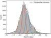 |
Fig. 8 Metallicity distribution of sample with six different Gaussian components plotted using different colours and representing the six sub-populations within Omega Cen. |
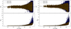 |
Fig. 9 Top: proper motions in RA (left) and Dec (right) as function of G-band magnitudes. Bottom: errors associated with proper motions in RA (left) and Dec (right) as function of G-band magnitude of the star. Stars in blue are taken from the Gaia FPR catalogue, and stars in yellow are taken from Gaia DR3. |
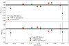 |
Fig. 10 Mean radial (top) and tangential (bottom) proper motions of the sub-populations obtained using AG24 (4 populations, red circles) and GMM (6 populations, green circles). The black line represents the mean values of proper motion calculated using Gaia DR3 stars. |
3.3 Rotation
An early study by Norris et al. (1997) analysed a sample of 400 RGB stars to understand the kinematical differences between the metal-rich and metal-poor populations. They used RVs from Mayor et al. (1997) and calcium abundances from Norris et al. (1996) to categorise the stars into two populations: metal-poor (80% of the total sample, [Ca/H] ≤ −1.2 dex) and metal-rich (20% of the sample, [Ca/H] > −1.2 dex). They found the metal-rich population to be more centrally located and kinematically cooler than the metal-poor population. Most importantly, they reported that the metal-poor population shows well-defined systemic rotation, whereas the metal-rich population is a nonrotating one (see Fig. 3 in their paper). Later, Pancino et al. (2007) looked at this rotation problem using high-resolution FLAMES spectra for about 650 RGB stars. They divided their sample into three populations (metal-rich, metal-intermediate and metal-poor). They found all the three populations to show the same rotational patterns. The measurement for the MR population, however, was based on a limited number of stars (only 70 stars, or about 11% of their sample) and presented a large scatter. Therefore, any signature of rotation that was being reported was associated with a large uncertainty.
We revisited the issue, taking advantage of our large sample (even for the metal-rich population) and conducted a similar analysis to Pancino et al. (2007). The first step was to calculate the position angle for all the stars within the sample as this would clearly represent the rotation with a sinusoidal variation. Once the position angles were obtained, we plotted it against the RVs obtained from the oMEGACat I catalogue as shown in Fig. 12. We made sure to only include reliable measurements for the RVs where the value was ≥ 3 σ and subtract the mean RV of the cluster from the individual measurements. The red curve in Fig. 12 is a non-linear fit obtained using χ2 minimisation. We clearly identify the sinusoidal variation in all of the four populations, implying the presence of rotational motion even in the most metal-rich population of Omega Cen. From the non-linear fitting, we estimate the amplitudes of the rotation velocities of the populations. Similarly to Pancino et al. (2007), we find rotational velocities to be uniform (as per Fig. 13) among the populations and the amplitudes to be around 6 km/s. The rotational velocities reported in Fig. 13 are only indicative values, as we expect stars with different radial distances to have different rotational values.
3.4 oMEGACat II
All the analysis mentioned above makes use of stars within the Gaia sample (FPR and DR3). As we already discussed, crowding is an issue in the central region of the cluster, due to which the Gaia sample had relatively few stars with accurate astrometry in the centre. To better probe the centre of the cluster we conducted the same analysis using HST data obtained from the oMEGACat II catalogue. This catalogue provides precise astrometry and multi-band photometry for over 1.5 million stars in the cluster’s core (covers a region of (0.2 × 0.2) deg around the centre; see Fig. 1). The astrometry in this catalogue is not only significantly better than that of Gaia FPR in terms of the uncertainties on the proper motions (see Fig. 12 of Häberle et al. 2024a), but it also includes stars ∼4 mag fainter than the faintest stars within the Gaia sample. The only limitation of this sample is its coverage, which is restricted to the very centre and does not include any stars from the outer regions of the clusters. Including some outer regions could allow for a comparison study between the inner and outer-region stars in terms of kinematics, as Norris et al. (1997) reported that the centrally concentrated metal-rich population was kinematically cooler.
We applied the same selection criteria to the HST astrometry as explained in Häberle et al. (2024a) and the same routine to obtain the cluster members. After the quality cuts, our high-quality sample had about 138 000 stars in it, which is an order of magnitude higher than what we had in the Gaia high-quality sample. We note that the relative HST proper motions were not converted into radial and tangential components as the oMEGACat II catalogue did not include the correlation metric between the two proper motions, which is essential for calculating the errors on the projections. The HST high-quality sample was then divided into four sub-populations using the bounds from AG24. The numbers of stars in MR, MIa, MIb, and MP populations are 2137, 15 517, 40 955, and 79 462, respectively. The percentage of stars within each population is similar to the one observed in the Gaia sample. Looking at the mean proper-motion values, even with a more precise dataset we do not find a significant difference in the motions of the populations as seen in Fig. 14. We did not perform the analysis using the GMM fitting as this was only intended to be a confirmation of the results obtained in the previous section.
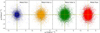 |
Fig. 11 Radial and tangential components of the proper motions of individual stars in the four populations obtained using AG24. The vertical and horizontal yellow lines represent the mean values of radial and tangential components of a particular population, respectively. The black dashed-vertical and horizontal lines represent the mean values of radial and tangential component of the metal-poor population. |
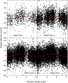 |
Fig. 12 Radial velocity plotted against position angle. The red line represents the best non-linear fit to the distribution. The sinusoidal variation represents the rotational motion within the populations. |
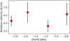 |
Fig. 13 Rotational velocity of four metallicity populations obtained using AG24. The values plotted above are the amplitudes of the nonlinear fitting shown in Fig. 12. |
3.5 Anisotropy
Anisotropy studies in GCs gain insight into their kinematics, and, when examined in terms of the different populations, they can potentially identify signatures of their formation process (Tiongco et al. 2016, 2019; Breen et al. 2017; Breen et al. 2021; Pavlík & Vesperini 2021, 2022; Vesperini et al. 2021). We follow the method described in Libralato et al. (2022) to probe the orbital anisotropies of the populations of Omega Cen. The analysis was limited to evolved stars with mF625m < 18.5 mag (including sub-giant branch and RGB stars). There are two reasons for this: the uncertainties on the radial and tangential proper motions are considerably larger for fainter MS stars, and the offset in the metallicities of the RGB with respect to the MS within the oMEGACat catalogue can lead to the mixing of the populations if using the RGB and the MS at the same time. We refined our sample by selecting stars with the highest quality proper-motion measurements: the top 20% of MIb and MP stars and the top 40% of MIa and MR stars (due to limited sample size) based on their uncertainties. The number of stars in MR, MIa, MIb, and MP were 893, 1279, 5030, and 9636, respectively, with number of bins within each population set to ten; therefore, each bin (except the last one) consisted of 89, 127, 503, and 963 stars, respectively. The velocity dispersion in radial and tangential directions within each bin was computed by maximising the likelihood of Eq. (1) in Libralato et al. (2022). The posterior distributions for σr and σt were obtained using a Markov chain Monte Carlo (MCMC) method through the emcee package (Foreman-Mackey et al. 2013) with 32 walkers, 5000 steps, and 500 steps as burn-ins. The normalised radial, tangential, and tangential-over-radial velocity dispersion as a function of radial distance is shown in Fig. 15 with the median of σt/σr for four populations in Fig. 16. All four populations show isotropy close to the centre, with MP showing a small radial anisotropy between 150 and 200 arcseconds and MIb being isotropic throughout. Between 200 and 300 arcsec, MIa shows tangential anisotropy, but close to 300 arcseconds all four populations seem to show isotropy again. Looking at the median value, MR, MIb, and MP show radial anisotropy, whereas MIa shows tangential anisotropy. However, all four populations show no significant differences among themselves, with all the values being within less than 2σ of each other.
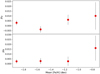 |
Fig. 14 Mean proper motion in RA (top) and Dec (bottom) of the four sub-populations obtained using stars from oMEGACat II catalogue based on HST observations. |
4 Discussion
Our understanding of the formation scenario of Omega Cen is still far from complete. The cluster is often cited as an extreme sample of the complexity of the multiple-population phenomenon in GCs, which has, however, an added degree of complexity: the MR population does not show the chemical trends and correlations that are the signatures of GC stars. Hypotheses of its origin have invoked accretion (either as an NSC or after being ingested into the Milky Way) or self-enrichment, with a pathway that must, however, have been different from that of the other populations. As the relaxation time of Omega Cen is relatively large for a GC, an ensamble of stars accreted by such a cluster would maintain its kinematical fingerprints for longer and, depending on how far in the past the event took place, be detectable in the motions of such a population. Our analysis of the motions of the different populations does not show significant differences with regard to the MR population. Interestingly, the Gaia proper motions for the MIa population seem to have a more discrepant value – even if still scarcely significant. This difference is not evident in the oMEGACat II data, which are, however, more centrally concentrated. This could possibly hint to the intriguing idea that an entire GC was captured by a proto-Omega Cen and that the fingerprints of its motions are still detectable in the outskirts of the cluster. The behaviour of the motions of the populations does not seem to be dependent on the metallicity bounds of the populations or on the number of populations, as the results from the six populations obtained through GMM fitting are also the same.
To probe the sensitivity of the motions on the metallicity bounds, we used a method similar to bootstrapping. We first randomly drew 50 000 values for each of the three metallicity bounds (as there are four populations in AG24) from three predefined Gaussian distributions. The peaks of these distributions are adopted from AG24, with the standard deviation being kept at 0.15 dex for all the three Gaussians. Once a set of metallicity bounds is randomly selected, these bounds were used to calculate the two mean proper motions for the four populations. With the motions calculated, we measured the largest proper motion difference among the four populations, and this difference is plotted in Fig. 17. It is clear that the largest differences are still quite small and are usually dominated by the error on the measurement. This is a clear indication that the number of populations and bounds of the populations have very little influence on the final mean motions of the populations, suggesting that the motions are uniform across the cluster.
Figure 10 shows how the uncertainties are quite large, especially on the most metal-rich population, due to small number of stars within it. The average error on the mean motions μr and μt is about 0.05 mas. For this reason, we also analysed the oMEGACat II catalogue, which is more precise in comparison to the Gaia sample. The average errors on the mean motions obtained using this catalogue are about 0.005 and 0.004 mas for μα and μδ, respectively (see Fig. 14). The measurements from oMEGACat II are an order of magnitude more precise than the Gaia measurements. Even with the increased precision, we do not see any significant difference among the motions of the populations, with the largest difference among the populations having a significance value of about 1σ. Similar results were found with the anisotropy analysis, with three of the populations showing radial anisotropy but no significant differences between each other.
The findings on the distribution and kinematics of stellar populations in Omega Cen align with the conclusions from Nitschai et al. (2024), which observed that the metallicity populations within the cluster’s half-light radius are well-mixed. This idea of well-mixed populations is further supported by the evidence of uniform rotation observed in this study. However, despite these insights, the main formation scenario of Omega Cen remains difficult to constrain due to the degeneracy between the properties of cluster stars formed through self-enrichment or through accretion, as in the latter, the stars could become kinematically integrated into the cluster.
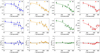 |
Fig. 15 Radial (top row), tangential (middle row), and tangential-over-radial (bottom panel) velocity dispersions for the four populations. The four populations MR, MIa, MIb, and MP are represented by blue, yellow, green, and red circles, respectively. The solid lines are the fourth-order polynomial fit to the velocity dispersion. The black line in the bottom panel represents isotropy, where tangential-over-radial velocity dispersion is equal to one. |
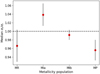 |
Fig. 16 Median value of tangential-over-radial velocity dispersion for the four metallicity populations. The dashed black line represents isotropy. |
5 Summary and conclusions
We present the kinematical analysis of stars within Omega Cen using the newly released Gaia FPR and DR3 data. The DR3 + FPR sample consists of about 520 000 stars, but this is reduced to about 28 000 stars after certain quality cuts were applied to ensure only high-quality measurements were used for the analysis. The first result we present regards the reliability of the Gaia FPR data. We find that a majority of Gaia FPR stars, either located in the central region or faint, are associated with large astrometric excess noise, due to which we lost about 90% of our sample. The main result of this work is that different metallicity populations exhibit the same mean proper motions, even after using a sample larger than that used in Sanna et al. (2020) and with the inclusion of main-sequence stars. This result is consistent with findings from Bellini et al. (2018), Libralato et al. (2018), and Sanna et al. (2020), which used lower quality data. The result is not influenced by the number of populations assigned or the metallicity bounds of the populations. The third result we present is evidence of rotation within all of the metallicity populations. They also have similar rotation amplitudes, which hints towards uniform rotation among all the stars.
Given the large uncertainties on the proper motions within the Gaia sample, we also analysed the HST sample from Häberle et al. (2024b). This new sample not only contains an order of magnitude more stars in each of the metallicity populations, but it is also significantly more precise than the Gaia sample. Despite all these facts, we do not see a significant difference in the mean proper motions. Therefore, from previous literature and results from this analysis, the possible conclusion we can obtain regarding the formation scenario is that the cluster is either formed through self-enrichment or though accretion, whereby the accreted population has completely integrated into the cluster. Future Gaia releases (i.e. Gaia DR4) are expected to yield higher quality measurements even in dense fields, such as in the interior of the cluster. Therefore, they might be able to provide further insight regarding the issue. Data from LSST will also help settle this debate in the future, given their expected high-quality proper motions for stars as faint as 27 mag in the V band.
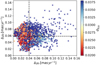 |
Fig. 17 Largest differences in the two proper motions of the four populations. The mean of the differences is shown by a dashed black line. The colour overlay represents the uncertainties on the largest differences in the radial component of the proper motion. |
Acknowledgements
This work has made use of data from the European Space Agency (ESA) mission Gaia (https://www.cosmos.esa.int/gaia), processed by the Gaia Data Processing and Analysis Consortium (DPAC, https://www.cosmos.esa.int/web/gaia/dpac/consortium). Funding for the DPAC has been provided by national institutions, in particular the institutions participating in the Gaia Multilateral Agreement. This job has made use of the Python package GaiaXPy, developed and maintained by members of the Gaia Data Processing and Analysis Consortium (DPAC), and in particular, Coordination Unit 5 (CU5), and the Data Processing Centre located at the Institute of Astronomy, Cambridge, UK (DPCI). PBK acknowledges support from the Japan Society for the Promotion of Science under the programme Postdoctoral Fellowships for Research in Japan (Standard). This work was supported by JSPS KAKENHI Grant Number JP23KF0290.
References
- Alfaro-Cuello, M., Kacharov, N., Neumayer, N., et al. 2019, ApJ, 886, 57 [Google Scholar]
- Alfaro-Cuello, M., Kacharov, N., Neumayer, N., et al. 2020, ApJ, 892, 20 [CrossRef] [Google Scholar]
- Alvarez Garay, D. A., Mucciarelli, A., Bellazzini, M., Lardo, C., & Ventura, P. 2024, A&A, 681, A54 [NASA ADS] [CrossRef] [EDP Sciences] [Google Scholar]
- Anderson, A. J. 1997, PhD thesis, University of California, Berkeley, USA [Google Scholar]
- Baumgardt, H., Hilker, M., Sollima, A., & Bellini, A. 2019, MNRAS, 482, 5138 [Google Scholar]
- Bedin, L. R., Piotto, G., Anderson, J., et al. 2004a, ApJ, 605, L125 [Google Scholar]
- Bellini, A., Piotto, G., Bedin, L. R., et al. 2009, A&A, 493, 959 [NASA ADS] [CrossRef] [EDP Sciences] [Google Scholar]
- Bellini, A., Anderson, J., Bedin, L. R., et al. 2017a, ApJ, 842, 6 [NASA ADS] [CrossRef] [Google Scholar]
- Bellini, A., Milone, A. P., Anderson, J., et al. 2017b, ApJ, 844, 164 [NASA ADS] [CrossRef] [Google Scholar]
- Bellini, A., Libralato, M., Bedin, L. R., et al. 2018, ApJ, 853, 86 [NASA ADS] [CrossRef] [Google Scholar]
- Breen, P. G., Varri, A. L., & Heggie, D. C. 2017, MNRAS, 471, 2778 [NASA ADS] [CrossRef] [Google Scholar]
- Breen, P. G., Rozier, S., Heggie, D. C., & Varri, A. L. 2021, MNRAS, 502, 4762 [Google Scholar]
- Calamida, A., Bono, G., Stetson, P. B., et al. 2009, ApJ, 706, 1277 [NASA ADS] [CrossRef] [Google Scholar]
- Callingham, T. M., Cautun, M., Deason, A. J., et al. 2022, MNRAS, 513, 4107 [NASA ADS] [CrossRef] [Google Scholar]
- Carretta, E., Bragaglia, A., Gratton, R. G., et al. 2010, A&A, 520, A95 [NASA ADS] [CrossRef] [EDP Sciences] [Google Scholar]
- Ester, M., Kriegel, H.-P., Sander, J., & Xu, X. 1996, in Second International Conference on Knowledge Discovery and Data Mining (KDD’96). Proceedings of a conference held August 2–4, eds. D. W. Pfitzner, & J. K. Salmon, 226 [Google Scholar]
- Ferraro, F. R., Bellazzini, M., & Pancino, E. 2002, ApJ, 573, L95 [Google Scholar]
- Foreman-Mackey, D., Hogg, D. W., Lang, D., & Goodman, J. 2013, PASP, 125, 306 [Google Scholar]
- Freeman, K. C., & Rodgers, A. W. 1975, ApJ, 201, L71 [NASA ADS] [CrossRef] [Google Scholar]
- Gaia Collaboration (Montegriffo, P., et al.) 2023a, A&A, 674, A33 [CrossRef] [EDP Sciences] [Google Scholar]
- Gaia Collaboration (Vallenari, A., et al.) 2023b, A&A, 674, A1 [NASA ADS] [CrossRef] [EDP Sciences] [Google Scholar]
- Gaia Collaboration (Weingrill, K., et al.) 2023c, A&A, 680, A35 [NASA ADS] [CrossRef] [EDP Sciences] [Google Scholar]
- Georgiev, I. Y., & Böker, T. 2014, MNRAS, 441, 3570 [Google Scholar]
- Häberle, M., Neumayer, N., Bellini, A., et al. 2024a, ApJ, 970, 192 [Google Scholar]
- Häberle, M., Neumayer, N., Seth, A., et al. 2024b, Nature, 631, 285 [CrossRef] [Google Scholar]
- Haywood, M., Di Matteo, P., Lehnert, M. D., et al. 2018, ApJ, 863, 113 [Google Scholar]
- Helmi, A., & White, S. D. M. 2001, MNRAS, 323, 529 [NASA ADS] [CrossRef] [Google Scholar]
- Helmi, A., Babusiaux, C., Koppelman, H. H., et al. 2018, Nature, 563, 85 [Google Scholar]
- Hesser, J. E., Bell, R. A., Cannon, R. D., & Harris, G. L. H. 1985, ApJ, 295, 437 [Google Scholar]
- Hughes, J., Wallerstein, G., van Leeuwen, F., & Hilker, M. 2004, AJ, 127, 980 [Google Scholar]
- Husser, T.-O., Latour, M., Brinchmann, J., et al. 2020, A&A, 635, A114 [NASA ADS] [CrossRef] [EDP Sciences] [Google Scholar]
- Ibata, R. A., Wyse, R. F. G., Gilmore, G., Irwin, M. J., & Suntzeff, N. B. 1997, AJ, 113, 634 [Google Scholar]
- Johnson, C. I., & Pilachowski, C. A. 2010, ApJ, 722, 1373 [NASA ADS] [CrossRef] [Google Scholar]
- Johnson, C. I., Dupree, A. K., Mateo, M., et al. 2020, AJ, 159, 254 [Google Scholar]
- Jönsson, H., Holtzman, J. A., Allende Prieto, C., et al. 2020, AJ, 160, 120 [Google Scholar]
- Kacharov, N., Alfaro-Cuello, M., Neumayer, N., et al. 2022, ApJ, 939, 118 [NASA ADS] [CrossRef] [Google Scholar]
- Kruijssen, J. M. D., Pfeffer, J. L., Reina-Campos, M., Crain, R. A., & Bastian, N. 2019, MNRAS, 486, 3180 [Google Scholar]
- Laporte, C. F. P., Johnston, K. V., Gómez, F. A., Garavito-Camargo, N., & Besla, G. 2018, MNRAS, 481, 286 [Google Scholar]
- Lee, Y. W., Joo, J. M., Sohn, Y. J., et al. 1999, Nature, 402, 55 [Google Scholar]
- Libralato, M., Bellini, A., Bedin, L. R., et al. 2018, ApJ, 854, 45 [NASA ADS] [CrossRef] [Google Scholar]
- Libralato, M., Bellini, A., Vesperini, E., et al. 2022, ApJ, 934, 150 [NASA ADS] [CrossRef] [Google Scholar]
- Limberg, G., Souza, S. O., Pérez-Villegas, A., et al. 2022, ApJ, 935, 109 [NASA ADS] [CrossRef] [Google Scholar]
- Massari, D., Koppelman, H. H., & Helmi, A. 2019, A&A, 630, L4 [NASA ADS] [CrossRef] [EDP Sciences] [Google Scholar]
- Mayor, M., Meylan, G., Udry, S., et al. 1997, AJ, 114, 1087 [Google Scholar]
- Mayer, L., Moore, B., Quinn, T., Governato, F., & Stadel, J. 2002, MNRAS, 336, 119 [CrossRef] [Google Scholar]
- Meylan, G., Mayor, M., Duquennoy, A., & Dubath, P. 1995, A&A, 303, 761 [NASA ADS] [Google Scholar]
- Neumayer, N., Seth, A., & Böker, T. 2020, A&A Rev., 28, 4 [NASA ADS] [CrossRef] [Google Scholar]
- Nitschai, M. S., Neumayer, N., Clontz, C., et al. 2023, ApJ, 958, 8 [Google Scholar]
- Nitschai, M. S., Neumayer, N., Häberle, M., et al. 2024, ApJ, 970, 152 [NASA ADS] [CrossRef] [Google Scholar]
- Norris, J. E., Freeman, K. C., & Mighell, K. J. 1996, ApJ, 462, 241 [NASA ADS] [CrossRef] [Google Scholar]
- Norris, J. E., Freeman, K. C., Mayor, M., & Seitzer, P. 1997, ApJ, 487, L187 [NASA ADS] [CrossRef] [Google Scholar]
- Pancino, E., Ferraro, F. R., Bellazzini, M., Piotto, G., & Zoccali, M. 2000, ApJ, 534, L83 [NASA ADS] [CrossRef] [Google Scholar]
- Pancino, E., Galfo, A., Ferraro, F. R., & Bellazzini, M. 2007, ApJ, 661, L155 [NASA ADS] [CrossRef] [Google Scholar]
- Pavlík, V., & Vesperini, E. 2021, MNRAS, 504, L12 [CrossRef] [Google Scholar]
- Pavlík, V., & Vesperini, E. 2022, MNRAS, 509, 3815 [Google Scholar]
- Pechetti, R., Kamann, S., Krajnović, D., et al. 2024, MNRAS, 528, 4941 [NASA ADS] [CrossRef] [Google Scholar]
- Pedregosa, F., Varoquaux, G., Gramfort, A., et al. 2011, J. Mach. Learn. Res., 12, 2825 [Google Scholar]
- Pfeffer, J., & Baumgardt, H. 2013, MNRAS, 433, 1997 [NASA ADS] [CrossRef] [Google Scholar]
- Pfeffer, J., Griffen, B. F., Baumgardt, H., & Hilker, M. 2014, MNRAS, 444, 3670 [NASA ADS] [CrossRef] [Google Scholar]
- Pfeffer, J., Lardo, C., Bastian, N., Saracino, S., & Kamann, S. 2021, MNRAS, 500, 2514 [Google Scholar]
- Platais, I., Wyse, R. F. G., Hebb, L., Lee, Y.-W., & Rey, S.-C. 2003, ApJ, 591, L127 [Google Scholar]
- Sanna, N., Pancino, E., Zocchi, A., Ferraro, F. R., & Stetson, P. B. 2020, A&A, 637, A46 [NASA ADS] [CrossRef] [EDP Sciences] [Google Scholar]
- Smith, V. V., Suntzeff, N. B., Cunha, K., et al. 2000, AJ, 119, 1239 [Google Scholar]
- Sollima, A., Ferraro, F. R., Pancino, E., & Bellazzini, M. 2005a, MNRAS, 357, 265 [NASA ADS] [CrossRef] [Google Scholar]
- Sollima, A., Pancino, E., Ferraro, F. R., et al. 2005b, ApJ, 634, 332 [NASA ADS] [CrossRef] [Google Scholar]
- Tiongco, M. A., Vesperini, E., & Varri, A. L. 2016, MNRAS, 461, 402 [NASA ADS] [CrossRef] [Google Scholar]
- Tiongco, M. A., Vesperini, E., & Varri, A. L. 2019, MNRAS, 487, 5535 [NASA ADS] [CrossRef] [Google Scholar]
- van de Ven, G., van den Bosch, R. C. E., Verolme, E. K., & de Zeeuw, P. T. 2006, A&A, 445, 513 [NASA ADS] [CrossRef] [EDP Sciences] [Google Scholar]
- van Leeuwen, F., Le Poole, R. S., Reijns, R. A., Freeman, K. C., & de Zeeuw, P. T. 2000, A&A, 360, 472 [NASA ADS] [Google Scholar]
- Vasiliev, E. 2019, MNRAS, 484, 2832 [Google Scholar]
- Vasiliev, E., & Baumgardt, H. 2021, MNRAS, 505, 5978 [NASA ADS] [CrossRef] [Google Scholar]
- Vesperini, E., Hong, J., Giersz, M., & Hypki, A. 2021, MNRAS, 502, 4290 [NASA ADS] [CrossRef] [Google Scholar]
- Villanova, S., Piotto, G., King, I. R., et al. 2007, ApJ, 663, 296 [NASA ADS] [CrossRef] [Google Scholar]
- Villanova, S., Geisler, D., Gratton, R. G., & Cassisi, S. 2014, ApJ, 791, 107 [Google Scholar]
Hubble Space Telescope.
Apache Point Observatory Galactic Evolution Experiment.
 .
.
All Tables
All Figures
|
Fig. 1 Distribution of stars observed by Gaia DR3 and Gaia FPR and oMEGACat II catalogue from Häberle et al. (2024a). Gaia FPR data are relatively more complete in the central region of Omega Cen in comparison to DR3, whereas oMEGACat II is complete in the very centre of the cluster. |
| In the text | |
|
Fig. 2 Distribution of Gaia EDR3 stars from Vasiliev & Baumgardt (2021) with membership probability ≥95%. The colour represents the number of stars within each hexbin. The black circle is the spacial region used to filter Gaia FPR stars. |
| In the text | |
|
Fig. 3 Distribution of proper motions in RA and Dec of all the Gaia FPR stars. Many stars have significantly larger proper motions than the mean proper motion of the cluster. The colour represents the number of stars within each hexbin. |
| In the text | |
|
Fig. 4 Left: CMD of all stars within our Gaia sample that match with the oMEGACat I catalogue. Right: CMD of stars that are included in the high-quality sample. |
| In the text | |
|
Fig. 5 Top: comparison between metallicities of oMEGACat I catalogue with that from AG24 (pink cross) and APOGEE (purple circles). The purple and pink dashed line represents the mean offset of AG24 and APOGEE from oMEGACat I metallicities, respectively. Bottom: comparison of radial velocities between oMEGACat I and APOGEE. The y-axes of the top and bottom panels represent [Fe/H]oMEGACatI − [Fe/H]lit and RVoMEGACatI − RVlit, respectively. |
| In the text | |
|
Fig. 6 Left: metallicity distribution of our sample with the one from AG24 shown in the inserted panel. Different metallicity populations are represented by different colours. Right: CMD of different sub-populations. |
| In the text | |
|
Fig. 7 Top: individual CMDs of populations from metal-rich ones in the leftmost panel to metal-poor ones in the rightmost panel. Bottom: mean metallicities of magnitude bins within different populations. |
| In the text | |
|
Fig. 8 Metallicity distribution of sample with six different Gaussian components plotted using different colours and representing the six sub-populations within Omega Cen. |
| In the text | |
|
Fig. 9 Top: proper motions in RA (left) and Dec (right) as function of G-band magnitudes. Bottom: errors associated with proper motions in RA (left) and Dec (right) as function of G-band magnitude of the star. Stars in blue are taken from the Gaia FPR catalogue, and stars in yellow are taken from Gaia DR3. |
| In the text | |
|
Fig. 10 Mean radial (top) and tangential (bottom) proper motions of the sub-populations obtained using AG24 (4 populations, red circles) and GMM (6 populations, green circles). The black line represents the mean values of proper motion calculated using Gaia DR3 stars. |
| In the text | |
|
Fig. 11 Radial and tangential components of the proper motions of individual stars in the four populations obtained using AG24. The vertical and horizontal yellow lines represent the mean values of radial and tangential components of a particular population, respectively. The black dashed-vertical and horizontal lines represent the mean values of radial and tangential component of the metal-poor population. |
| In the text | |
|
Fig. 12 Radial velocity plotted against position angle. The red line represents the best non-linear fit to the distribution. The sinusoidal variation represents the rotational motion within the populations. |
| In the text | |
|
Fig. 13 Rotational velocity of four metallicity populations obtained using AG24. The values plotted above are the amplitudes of the nonlinear fitting shown in Fig. 12. |
| In the text | |
|
Fig. 14 Mean proper motion in RA (top) and Dec (bottom) of the four sub-populations obtained using stars from oMEGACat II catalogue based on HST observations. |
| In the text | |
|
Fig. 15 Radial (top row), tangential (middle row), and tangential-over-radial (bottom panel) velocity dispersions for the four populations. The four populations MR, MIa, MIb, and MP are represented by blue, yellow, green, and red circles, respectively. The solid lines are the fourth-order polynomial fit to the velocity dispersion. The black line in the bottom panel represents isotropy, where tangential-over-radial velocity dispersion is equal to one. |
| In the text | |
|
Fig. 16 Median value of tangential-over-radial velocity dispersion for the four metallicity populations. The dashed black line represents isotropy. |
| In the text | |
|
Fig. 17 Largest differences in the two proper motions of the four populations. The mean of the differences is shown by a dashed black line. The colour overlay represents the uncertainties on the largest differences in the radial component of the proper motion. |
| In the text | |
Current usage metrics show cumulative count of Article Views (full-text article views including HTML views, PDF and ePub downloads, according to the available data) and Abstracts Views on Vision4Press platform.
Data correspond to usage on the plateform after 2015. The current usage metrics is available 48-96 hours after online publication and is updated daily on week days.
Initial download of the metrics may take a while.