| Issue |
A&A
Volume 695, March 2025
|
|
|---|---|---|
| Article Number | A265 | |
| Number of page(s) | 15 | |
| Section | Extragalactic astronomy | |
| DOI | https://doi.org/10.1051/0004-6361/202453315 | |
| Published online | 25 March 2025 | |
Investigating AGN feedback in Hα-luminous galaxy clusters: First Chandra X-ray analysis of Abell 2009
1
Scuola Universitaria Superiore IUSS Pavia, Palazzo del Broletto, Piazza della Vittoria 15, I-27100 Pavia, Italy
2
Department of Physics, University of Trento, Via Sommarive 14, I-38123 Povo, (TN), Italy
3
Dipartimento di Fisica e Astronomia, Università di Bologna, Via Gobetti 93/2, 40129 Bologna, Italy
4
Istituto Nazionale di Astrofisica (INAF) – Istituto di Radioastronomia (IRA), Via Gobetti 101, I-40129 Bologna, Italy
⋆ Corresponding author; ilaria.fornasiero@iusspavia.it
Received:
5
December
2024
Accepted:
22
February
2025
Aims. We analyze the X-ray and radio properties of the galaxy cluster Abell 2009 (z ∼ 0.152) to complete the in-depth individual study of a subsample of objects from the ROSAT Brightest Cluster Sample (BCS) with a relatively high X-ray flux and Hα line luminosity, which is a promising diagnostic of the presence of cool gas in the cluster cores. Our aim is to investigate the feedback from the active galactic nucleus (AGN) in the central galaxy and the intracluster medium (ICM) of relaxed clusters.
Methods. In this work, we analyze archival data from JVLA and Chandra observations. We performed a morphological analysis of both the X-ray emission from the ICM of Abell 2009 and of the radio emission from the AGN in the central galaxy. We also performed a spectral analysis of the X-ray emission, to derive the global properties and radial profiles of the thermal gas.
Results. Our X-ray analysis confirms the expectations, based on the selection criteria, that Abell 2009 is a cool-core system. We estimate a cooling radius of ∼88 kpc within which the ICM is radiating away its energy at rates of Lcool ∼ 4.4 × 1044 erg s−1. Radio observations of the central galaxy reveal a bright core surrounded by radio lobes on 30 kpc scales, with a symmetric butterfly-shaped morphology. We also present the detection of an extended radio galaxy to the northwest of the central one that is also a cluster member of Abell 2009. Although we did not detect any clear X-ray cavity at the position of the central radio lobes by assuming that their size is comparable, we combined the volume of the lobes with the pressure of the surrounding ICM to derive the work done by the AGN on the gas to inflate them. By estimating a cavity age of about 20 Myr, this corresponds to a mechanical power of ≈1045 erg s−1, which is sufficient to counterbalance the radiative cooling losses in Abell 2009. We finally discuss possible correlations between the global properties of the 18 objects from the BCS selection, finding in particular that the number of outbursts required to counterbalance the radiative ICM losses is linearly anticorrelated with the energetics and power of the outburst.
Key words: methods: observational / radio continuum: galaxies / X-rays: galaxies: clusters
© The Authors 2025
 Open Access article, published by EDP Sciences, under the terms of the Creative Commons Attribution License (https://creativecommons.org/licenses/by/4.0), which permits unrestricted use, distribution, and reproduction in any medium, provided the original work is properly cited.
This article is published in open access under the Subscribe to Open model. Subscribe to A&A to support open access publication.
1. Introduction
Within galaxy clusters, the majority of the baryonic component is in the form of a hot, diffuse gas permeating the cluster’s volume, known as the intracluster medium (ICM). This gas emits strongly in X-rays at temperatures of T ∼ 107 − 108 K (corresponding to a few keV1), primarily through thermal bremsstrahlung radiation and with typical luminosities around LX ∼ 1044 erg s−1 (see Sarazin 1986).
Nowadays, galaxy clusters are broadly classified into two main categories: cool-core and non cool-core. Cool-core clusters are characterized by a decreasing temperature profile toward the center and a dense (electron density ne ∼ 10−2 cm−3) core. On the other hand, non cool-core clusters do not show signs of a lower central temperature and higher central density, and they generally show evidence of recent dynamical activity, such as minor or major mergers (e.g., Markevitch & Vikhlinin 2007; Rossetti & Molendi 2010).
Focusing on cool-core systems, the relevance of radiative losses coming from the emission of the hot ICM can be established by considering its characteristic cooling time. In the central regions of cool-core clusters, where the cooling time (tcool ∝ kT/ne) is typically below a few gigayears, the ICM experiences a sufficiently high cooling rate, leading to the dissipation of particles’ energy through X-ray radiation. Early studies of the cores of galaxy clusters predicted the emergence of a cooling flow of material toward the center of the cluster (see Fabian 1994). Nonetheless, later studies have shown that the net rate of gas actually cooling to low temperatures is only 1−10% of the classical expected cooling flow rate (e.g., David et al. 2001; Peterson & Fabian 2006). Historically, there have been two primary strategies to address the inconsistency of the so-called cooling flow problem. As the gas emits radiation without signs of cooling, either the typical signatures of radiative cooling below 1−2 keV are somehow inhibited (e.g., Fabian et al. 2001, 2022; Morris & Fabian 2003; Mathews & Brighenti 2003) or a mechanism injecting energy into the ICM must exist to counterbalance the cooling process (e.g., Markevitch et al. 2001; Voigt et al. 2002; Domainko et al. 2004; McNamara & Nulsen 2007; Gaspari et al. 2012). Regarding the latter, it has been recognized that central galaxies – also known as brightest cluster galaxies (BCGs) – in cool-core clusters show a prevalence of radio activity (Best et al. 2007). In ∼70% of cases, the BCGs hosting an active galactic nucleus (AGN) were associated with Fanaroff-Riley type I (FRI) radio galaxies (see Fanaroff & Riley 1974; Burns 1990). FRI radio galaxies are center-brightened showing more luminous and irregular jets in the central parts and faint lobes at the edges (Banfield et al. 2015). From Chandra telescope images, the central hot gas in numerous cool-core systems exhibits a nonuniform distribution that closely aligns with the extended lobes of radio emission (e.g., Blanton et al. 2001; Fabian et al. 2003). These observations also unveiled different structures within the cores of many clusters, such as shocks, ripples, and abrupt density variations. A comparison with radio images suggested that many of these disturbances are associated with the activity of AGN jets. The propagation of the jets displaces the X-ray-emitting gas in the cluster atmosphere, excavating depressions in the ICM that manifest as cavities in X-ray images (e.g., Bîrzan et al. 2004; McNamara & Nulsen 2007; Gitti et al. 2012). These structures are currently regarded as an extremely powerful tool to demonstrate that the mechanical power of the AGN is capable of heating the ICM (e.g., Brighenti & Mathews 2006; Bîrzan et al. 2008; Gaspari et al. 2012). Multiple comparisons over the years of the cavity power, Pcav, and the bolometric X-ray luminosity of the cooling region, Lcool, have indeed shown a consistent scaling between the two quantities (e.g., Bîrzan et al. 2004, 2012; Rafferty et al. 2006; Olivares et al. 2022; Ubertosi et al. 2023a). This suggests that, on average, the mechanical power of the jets is able to offset the radiative cooling losses of the ICM. As multiple AGN outbursts can occur within a cooling time of the ICM (few hundreds of million years), the exact balance between the AGN heating power and the ICM cooling losses also depends on the duty cycle of the AGN, which is the fraction of time during which the central supermassive black hole (SMBH) is actively driving relativistic jets through its surrounding environment (see Rafferty et al. 2008; Best & Heckman 2012; Gitti et al. 2012).
In addition to the effects of AGN activity, sloshing motions are frequently observed in the cores of cool-core clusters. Sloshing arises from gravitational perturbations in the potential wells, typically caused by minor mergers or interactions, and manifests as spiral structures in the X-ray surface brightness and temperature maps (e.g., Markevitch & Vikhlinin 2007; ZuHone et al. 2010). These motions redistribute the energy within the ICM, which impacts the thermodynamic state of the gas. Sloshing can influence cooling by generating thermal instabilities, which play a key role in regulating the distribution and cooling rates of the ICM. At the same time, it can affect the co-spatiality between the AGN and its fuel reservoirs, potentially destabilizing the AGN feedback cycle. Early studies suggest that sloshing does not break the feedback loop, but may influence the timing and efficiency of the AGN activity (e.g., Pasini et al. 2021; Rosignoli et al. 2024).
Several optical (e.g., McDonald et al. 2010) and submillimeter (e.g., Edge 2001) observations of BCGs have revealed the presence of warm and cold gas filaments, likely cooling out of the ICM and spatially connected to the core of the BCG, which are thought to ultimately provide the fuel for the SMBH (see Hamer et al. 2016; Olivares et al. 2019; Gaspari et al. 2020; Donahue & Voit 2022). In this context, studying systems with strong Hα emission and high X-ray flux is essential to understand the feeding and feedback cycle in cool-core clusters, as these features are typical of systems where both cooling and heating processes are most likely at play (e.g., Ettori et al. 2013). The AGN-ICM interaction is, in fact, two-fold: not only do the relativistic jets heat the gas, but the gas itself can provide fuel to sustain the AGN activity. This two-fold interplay is known as the self-regulated feedback loop (see McNamara & Nulsen 2007; Fabian 2012), where hot gas cooling initially triggers the SMBH activity (e.g., Ubertosi et al. 2023b), leading to relativistic jets depositing mechanical energy into the gas and reducing further cooling; as the jet activity weakens, more efficient cooling is restored (see Gaspari et al. 2011; Li et al. 2015 for numerical simulations).
This work aims to complete the study of individual targets from a selection of galaxy clusters that are expected to be exemplary cases of the self-regulated feedback loop. As previously discussed in Ettori et al. (2013), Pasini et al. (2019, 2021), Ubertosi et al. (2023c), Rosignoli et al. (2024), the conditions that regulate the interaction between AGN feedback and ICM cooling can be best explored in systems with a relatively high X-ray flux and a BCG that is relatively bright in the Hα line (suggesting the presence of cool gas). The above previous works selected systems from the ROSAT Brightest Cluster Sample (BCS) of 201 galaxy clusters with X-ray fluxes greater than 4.4 × 10⁻¹² erg cm−2 s−1 (Ebeling et al. 1998) and Hα luminosities greater than 1040 erg s−1 (Crawford et al. 1999). The resulting 18 objects are reported in Table 1, and we refer the reader to Ubertosi et al. (2023c) for a short summary on the properties of these systems. We note that the BCS catalog and the work of Crawford et al. (1999) are restricted to the northern sky. This makes the selected systems visible from the Jansky Very Large Array (JVLA), which has been routinely used to investigate the properties of radio galaxies at the center of clusters (e.g., Bîrzan et al. 2008). A similar selection in the southern sky, where other radio telescopes such as MeerKAT and Australian Square Kilometer Array Pathfinder (ASKAP) could be used to perform a similar analysis, will be the aim of future works.
Selection of high X-ray flux and high Hα luminosity galaxy clusters from the BCS sample.
The majority of the galaxy clusters from this selection (listed in Table 1) have at least one dedicated study in the literature (e.g., Sun et al. 2003; McNamara et al. 2006; Blanton et al. 2011; Pandge et al. 2013; Sonkamble et al. 2015; Vantyghem et al. 2016; Russell et al. 2017), which confirmed the expectation that these objects are representative examples of the interplay between the AGN and the ICM. These dedicated studies typically employed Chandra observations of the ICM, to spatially resolve the evidences of feedback (e.g., the cavities), and JVLA observations of the central radio galaxy. For example, ZwCl 1742 shows evidence of cold fronts and a weak shock in Chandra data, suggesting the presence of sloshing gas in the cluster core or a metal-rich outflow from the central AGN (Ettori et al. 2013). Abell 2495 shows an offset between the BCG and the X-ray emission peak, and a potential sloshing-induced activation of the central AGN, which emphasizes the key role of the sloshing effect on the self-regulated feedback loop (Pasini et al. 2019; Rosignoli et al. 2024). Recent works also include the study of Abell 1668 (Pasini et al. 2021) and ZwCl 235 (Ubertosi et al. 2023c), which show important signs of the AGN feedback cycle regulating the cooling process and the presence of a possible sloshing phenomenon in these galaxy clusters.
The only cluster in this selection (see Table 1) that still lacks a dedicated study is Abell 2009 (z = 0.152), located at RA: 15:00:19.52 and Dec: +21:22:09.90. Its Hα luminosity is relatively small (≈6 × 1040 erg s−1) compared to other well-studied clusters at the top of Table 1, indicating a small star formation rate (which is also evident from the low upper limit of infrared luminosity given by Quillen et al. 2008).
The aim of the present work is to perform a detailed analysis of Abell 2009 by means of archival Chandra (20 ks) and JVLA (45 minutes) observations, in order to investigate its dynamical state and emission properties, and derive, for the first time, a comprehensive picture of the AGN feeding and feedback cycle within the systems. As the study of this cluster completes the dedicated investigation of the 18 objects in the BCS subsample (see Table 1), we also aim at providing a general overview of how heating and cooling proceeds in these representative examples of cool-core systems.
In this work, a ΛCDM cosmology is assumed, with H0 = 70 km s−1 Mpc−1, Ω0 = 0.3, and ΩΛ = 0.7. At the cluster redshift (z = 0.152), the angular size distance DA is 545.8 Mpc, the luminosity distance DL is 724.6 Mpc, and the scale corresponds to 2.65 kpc/″.
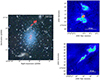 |
Fig. 1. Multiwavelength view of Abell 2009. Left panel: In this image, the radio emission at 1.5 GHz observed with the JVLA telescope and the X-ray emission detected by the Chandra telescope are shown in red and blue, respectively. Both emissions are overlaid on an optical image from the DESI survey for a comprehensive view of the system. Upper right panel: 1.5 GHz JVLA radio image zoomed on the BCG, at a resolution of 1.2″ × 1.1″. The rms value is σrms = 19 μJy/beam. Magenta contour levels are taken at 3, 6, 12, 24 × σrms. Lower right panel: 1.5 GHz JVLA radio image zoomed on the northern radio galaxy, at a resolution of 1.2″ × 1.1″. The rms value is σrms = 19 μJy/beam. Magenta contour levels are taken at 3, 6, 12, 24 × σrms. |
2. Data and methods
2.1. Chandra X-ray data
Abell 2009 was observed with the Chandra telescope during the Cycle 10 (ObsID 10438) for an exposure time of 19.9 ks. The data were acquired using ACIS-I instrument in VFAINT mode. The data reduction has been performed with the CIAO(v4.15) software (Chandra Interactive Analysis of Observations, Fruscione et al. 2006) and the calibration data CALDB(v4.10.2). In order to reprocess the data, the chandra_repro script was used. The astrometry correction was performed by cross-matching the point sources (detected using the tool wavdetect) with two different catalogs: the United States Naval Observatory (USNO-A2.0) and the Gaia Data Release 2 (Gaia-DR2) optical catalogs. The best correction is achieved by using Gaia-DR2 catalog, owing to its high spatial resolution of ∼200 mas (Gaia Collaboration 2018), compared with the ∼250 mas resolution of USNO-A2.0 catalog. The final astrometric correction on the Chandra dataset is of 1.3″ in the horizontal direction and −0.6″ in the vertical direction. The data were filtered to exclude time intervals with background flares. After running the deflare task, the cleaned exposure is 17.3 ks (87% of the original exposure). The blank-sky script was used to automatically identify the appropriate blank-sky background file, which was subsequently normalized by the 9−12 keV count rate of the observation.
In order to investigate the X-ray morphology of the ICM, the target, exposure and background images were produced in the 0.5−7 keV energy range. From these images, surface brightness radial profiles were extracted and fitted using Sherpa. The spectral analysis was performed using the Xspec(v.12.13.0c) software. The spectra were fitted in the energy range 0.5−7 keV and grouped with at least 25 counts in each spectral bin, enough to apply the χ2 statistic. Each spectrum is associated with ancillary response files (ARFs) and response matrix files (RMFs), and the blank-sky background spectrum is subtracted. The weight parameter is set to yes, which spatially weights the source ARF, as appropriate for extended sources. Moreover, the point sources are excluded from each region selected, in order to avoid contamination to the thermal spectra of the ICM. For every model used, we included a tbabs model component, representing galactic absorption due to the medium interposed between the source and the observer. The column density of galactic neutral hydrogen has been fixed to NH = 3.18 × 1020 cm−2 (HI4PI Collaboration 2016). Moreover, we adopted the table of solar abundances from Asplund et al. (2009).
2.2. JVLA radio data
To complement the X-ray analysis of Abell 2009, we considered radio observations that could provide radio maps with a resolution comparable to that of Chandra (⪅1″) and good sensitivity to extended emission from radio galaxies in the cluster. To this end, we consider the JVLA observations at L band (1−2 GHz) with the A configuration (∼1″ resolution), performed in 2014 (project 14A-280). The primary calibrator for this observation is 1331+305 = 3C286, while the secondary calibrator is J1513+2338. The target Abell 2009 was observed for 45 minutes. The data were calibrated using CASA v.6.4.1 (CASA Team 2022) following standard data reduction procedures for continuum observations2. We attempted self-calibration of the target, but its relatively low peak flux density (about 6 mJy at 1.5 GHz) prevented us from obtaining useful phase and amplitude solutions. In any case, the rms noise of our images (about 20 μJy/beam) is close to the theoretical expected one (about 15 μJy/beam). Images were obtained in CASA with the task tclean adopting multiscale cleaning and multifrequency synthesis. We found that imaging with robust = 0.5 offers the best compromise between spatial resolution and sensitivity to extended emission. Uncertainties on the measured flux densities were obtained using the equation
where S is the flux density, Nbeam is the number of beams in the source area, and σc is the systematic calibration error on the flux, which is typically assumed of 5% for JVLA (Condon et al. 1998).
3. Results
In this section, we outline the results of the morphological and spectral analysis of Abell 2009.
3.1. Radio morphological analysis
In Fig. 1 (left panel), we present the 1.5 GHz JVLA radio emission (in red) and the Chandra X-ray emission (in blue) of Abell 2009, overlaid on an optical image for a multiwavelength view of the system. The image reveals the radio emission of two different sources: the radio galaxy associated with the BCG and another radio galaxy in the north direction. The BCG emission presents a bright core and extended radio lobes (∼17 kpc long), oriented from northwest (NW) to southeast (SE), which are symmetrically distributed in a butterfly-shaped morphology (see Fig. 1 upper right panel). The arched and concave morphology of the lobes may be caused by precession of the jets around their axis, by projection effects, or both (e.g., Sternberg & Soker 2008; Wong et al. 2008; Hlavacek-Larrondo et al. 2013). We measured that this radio galaxy has a total flux density of 23 ± 1.0 mJy above 3σ level, with 5.8 ± 0.3 mJy coming from the central bright core (see Table 2). The radio powers at 1.5 GHz are calculated assuming a spectral index3α = −1 for the BCG (Kimball & Ivezić 2008) and α = −0.3 for the core component (Hogan et al. 2015), using the formula:
Properties of the radio sources in Abell 2009.
Their estimates are (1.45 ± 0.06)×1024 W Hz−1 and (0.33 ± 0.02)×1024 W Hz−1, respectively (see Table 2). Considering its morphology and the radio power value, this galaxy can be associated to an FRI type (see Ledlow & Owen 1996).
The radio galaxy in the N direction, located approximately at 50″ from the BCG, presents an elongated radio lobe and, along the direction of the lobe toward SE, a compact core can be observed (see Fig. 1 lower right panel), which corresponds to an elliptical galaxy at the same redshift of the cluster (2MASX J15002058+2122548, z = 0.157 from Ahumada et al. 2020). Thus, this radio galaxy is a cluster member of Abell 2009 and has a total flux density of 41.0 ± 1.6 mJy (including the core emission), corresponding to a 1.5 GHz radio power of (2.77 ± 0.11)×1024 W Hz−1, calculated assuming α = −1 (see Table 2).
3.2. X-ray morphological analysis
In this section, we describe the X-ray surface brightness profile extraction and the fit with both a single β model and a double β model. Subsequently, we describe the 2D fitting analysis, deriving the residual image used to investigate the presence of ICM substructures.
3.2.1. Surface brightness profile
In Fig. 2, we show the 0.5−7 keV Chandra image of Abell 2009. The azimuthally averaged surface brightness profile is extracted with CIAO. The extraction regions are concentric circular annuli centered on the BCG coordinates, which is located at the X-ray peak at the center of the cluster. The annuli extend to a maximum radius of 131″ (∼347 kpc) and are spaced with a 1″ width, except for the outermost three that are wider (≈4″) to include more counts. The emission from the X-ray point sources across the field was excluded, as well as the innermost 2 bins of the profile, where contamination from the AGN in the BCG may be present.
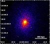 |
Fig. 2. 0.5−7 keV Chandra image of the galaxy cluster Abell 2009, convolved with a Gaussian function of a 2 pixel radius. |
Single and double β model fits.
Initially, the surface brightness profile is fitted with a single β model (Cavaliere & Fusco-Femiano 1978) defined as:
![$$ \begin{aligned} S(r) = A \left[1+\left(\frac{r}{r_0}\right)^2\right]^{0.5-3\beta }, \end{aligned} $$](/articles/aa/full_html/2025/03/aa53315-24/aa53315-24-eq3.gif)
where A is the amplitude of the model, r0 is the core radius, and β is the parameter that controls the slope of the profile at large radii. The best-fit parameters are reported in Table 3 and the fitted profile in Fig. 3. As it can be seen from the profile, the model does not fit accurately the surface brightness in the central regions, where there is an evident excess of emission. This discrepancy is a characteristic feature of cool-core clusters, where the denser cores undergo radiative cooling and exhibit elevated X-ray luminosity (e.g., Lewis et al. 2003). Moreover, the reduced χ2 value is 322.9/115 = 2.8, meaning that the model cannot properly represent the data.
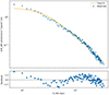 |
Fig. 3. 0.5−7 keV surface brightness profile of Abell 2009 fitted with a single β model. The lower subplot represents the residuals in σ units. |
To properly describe the surface brightness profile, we fitted it with a double β model, defined as:
![$$ \begin{aligned} S(r) = A_1 \left[1+\left(\frac{r}{r_{0,1}}\right)^2\right]^{0.5-3\beta _1} + A_2 \left[1+\left(\frac{r}{r_{0,2}}\right)^2\right]^{0.5-3\beta _2}, \end{aligned} $$](/articles/aa/full_html/2025/03/aa53315-24/aa53315-24-eq4.gif)
where A1 and A2 are the amplitudes, r0, 1 and r0, 2 are the core radii, and β1 and β2 are the parameters that controls the slopes of each component. The fit is performed both by considering different values for the two β (Ettori 2000) and by linking them to the same value (Mohr et al. 1999). The best-fit parameters of both cases are reported in Table 3 and their respective fitted profiles in Fig. 4.
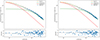 |
Fig. 4. Left panel: 0.5−7 keV surface brightness profile of Abell 2009 fitted with a double β model where the values of β are unlinked (see Table 3). The orange line represents the total model, while the red and green lines correspond to the two components of the model. The lower subplot represents the residuals in σ units. Right panel: 0.5−7 keV surface brightness profile of Abell 2009 fitted with a double β model where the values of β are linked (see Table 3). The orange line represents the total model, while the red and green lines correspond to the two components of the model. The lower subplot represents the residuals in σ units. |
From the reduced χ2 values in Table 3, it is clear that this model better fits the data compared to the single β model. The fit in which the two β values were linked (see Table 3, last row) yields best-fit parameters and statistics that are consistent with the case of different β values (see also e.g., Rosignoli et al. 2024). For this reason, it is reasonable to consider the model with the linked β values as the best fit to the data.
3.2.2. Searching for X-ray cavities
In order to investigate the possible presence of substructures in the ICM, we derived a residual (model subtracted) image of the X-ray emission from Abell 2009. Specifically, the 0.5−7 keV image of Abell 2009, subtracted from the background and corrected by the exposure, is fitted with a 2D double β model in Sherpa. The extraction region corresponds to the largest possible circle centered in the BCG coordinates with a radius of 131″ (∼347 kpc). The free parameters of the fit are the core radius, r0, the ellipticity of the model, ellip ( , where a is the semi-major axis and b is the semi-minor axis of the ellipse), the angle of the major axis, theta, the amplitude of the model, ampl, and the power-law slope of the profile at large radii, δ. The slope β of the single power-law model directly relates to the brightness profile, while the slope δ of the double power-law corresponds to the exponent (0.5−3β) of Eq. (3) and by equating the two expressions, the following relationship is obtained: β = (δ + 0.5)/3. The best-fit parameters are reported in Table 4.
2D double β model fit.
In Fig. 5, we show the residual image derived by subtracting the 2D fit from the original Chandra image, with the radio contours at 1.5 GHz superimposed. The comparison between the residual map and the radio contours shows no clear evidence of depressions in the ICM that align with the radio lobes. We further evaluated the significance of several negative residual patches visible in the image, but none were found to be statistically significant. However, we note that this does not necessarily imply the absence of cavities. Given the short exposure time of the Chandra observations (∼17 ks), potential cavities may not be detectable at the current sensitivity level. In order to evaluate any feedback effect from this radio galaxy on the ICM, in the following we consider the radio lobe volumes as tracers of the mechanical energy injected by the AGN jets, as previously done in the literature in other cases where cavities were not detected in X-rays (e.g., Timmerman et al. 2022; Seth et al. 2022).
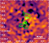 |
Fig. 5. Residual image of the best-fit double β model convolved with a Gaussian function of a 5 pixel radius. The green contours identify the radio emission at 1.5 GHz. The rms noise is σrms = 19 μJy/beam. The contour levels start from 3σ and increase by a factor 2, while the beam size is 1.2″ × 1.1″. The black cross corresponds to the position of the BCG. |
We also searched for possible surface brightness edges in Abell 2009 that could trace cold fronts or shocks. However, we could not confirm the presence of any significant density jump in the existing Chandra observations. While it is possible that the cluster does not currently host cold or shock fronts, it is also possible that the relatively short Chandra exposure of 20 ks is not deep enough to reveal shallow and localized gradients in surface brightness.
3.3. X-ray spectral analysis
In this section, we describe the global spectral extraction performed to obtain the large-scale properties of the cluster Abell 2009. Subsequently, we outline the methods to perform a thorough projected and deprojected analysis. The latter is essential to provide an effective representation of the thermodynamical radial profiles of the ICM and, consequently, to understand the dynamical state of the gas.
3.3.1. Global spectral properties of Abell 2009
To derive a global spectrum of the ICM and measure the basic thermodynamic properties, such as temperature and metallicity, we considered an ellipse centered on the BCG with a semi-major axis of 164″ (∼434 kpc), a semi-minor axis of 130″ (∼343 kpc), and an inclination angle of 77.3°. This extraction region corresponds to the largest area that can be covered within the Chandra field of view. The regions of the point sources are excluded from the global spectral analysis. The fit of the spectrum is performed using a tbabs*apec model, which includes the component of galactic absorption of the medium interposed between the source and the observer (tbabs), and the one of thermal emission (apec). The second component accounts for the thermal emission from a collisional ionized gas, with parameters of temperature kT, metal abundance Z, redshift z, and normalization norm of the spectrum. The spectrum is then fitted with this model and the results are shown in Table 5. The best-fit parameters are kT = 6.41 ± 0.17 keV and Z = 0.59 ± 0.07 Z⊙, which are consistent with the typical values of galaxy clusters (Bahcall 1996).
Global spectrum best-fit of Abell 2009.
3.3.2. Projected radial analysis
This analysis is performed to derive the profiles of the projected thermodynamical quantities. The spectra are extracted from eight elliptical and concentric annuli, centered in the coordinates of the BCG. The spacing between the annuli is determined by the requirement that inside each annulus there must be at least 2000 net counts, in order to accurately constrain the fit parameters. The annuli are chosen with the same ellipticity and inclination angle of the surface brightness distribution of the cluster (see Sect. 3.2.2). The maximum extension is an ellipse with a semi-major axis of 164″ (∼434 kpc) and a semi-minor axis of 130″ (∼343 kpc). Furthermore, the central 1.5″ (∼4 kpc) have not been considered, since any contribution from the X-ray emission of the AGN may contaminate the ICM spectrum in that region. Each annulus spectrum is fitted with a tbabs*apec model and the results are shown in Table A.1. In Fig. 6, we show the projected temperature profile. As it can be observed, the temperature decreases going toward small radii, which is typical of cool-core clusters (Peterson & Fabian 2006).
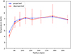 |
Fig. 6. Projected (blue) and deprojected (red) radial temperature profiles of Abell 2009. The temperature measurements are reported in Tables A.1 and 6. |
3.3.3. Deprojected radial analysis
In the projected analysis, the derived quantities suffer from the contribution of the ICM from the outer regions that is projected along the line of sight and the normalization parameter cannot be used to calculate the electron density in each annulus. The deprojection analysis is performed in order to obtain radial quantities without the influence of the projection effect. The same spectra used for the projected analysis were loaded on Xspec and fitted with a projct*tbabs*apec model. The projct mixing model component performs a 3D to 2D projection of prolate ellipsoidal shells onto elliptical annuli. The best-fit results are listed in Table 6 and, in Fig. 6, we show the deprojected temperature profile superimposed to the corresponding projected profile.
Best-fit parameters of the deprojected radial spectral analysis of Abell 2009.
The deprojected profile is broadly consistent with the projected one, showing a central decrease in temperature and a flat profile at r ⪆ 100 kpc. The central temperature drop appear slightly more pronounced than in the projected profile, although the larger uncertainties associated with the more complex deprojection model prevent any meaningful comparison. Using the normalization values of the deprojected analysis, we calculated the electron density of the plasma for each annulus. The normalization is defined as:
![$$ \begin{aligned} \mathrm{norm}=\frac{10^{-14}}{4\pi [D_{\rm A}(1+z)]^2} \int n_{\rm e} n_{\rm H} \mathrm{d}V, \end{aligned} $$](/articles/aa/full_html/2025/03/aa53315-24/aa53315-24-eq38.gif)
where DA is the angular distance from the source (DA = 545.8 Mpc for Abell 2009), z is the redshift, ne and nH are the electron and proton densities, and V is the volume of the emitting region. It is possible to invert this equation and derive the electron density:
![$$ \begin{aligned} n_{\rm e}=\sqrt{10^{14}\left(\frac{4\pi \times \mathrm{norm} \times [D_{\rm A} (1+z)]^2}{0.83V}\right)}\cdot \end{aligned} $$](/articles/aa/full_html/2025/03/aa53315-24/aa53315-24-eq39.gif)
The electron density values for each annulus are reported in Table 6 and its profile in Fig. 7 (upper left panel). Subsequently, the pressure and entropy profiles were calculated from the density profile, assuming ne ≈ 1.2np and using the following formulae: p = 1.83 nekT and  . The best-fit values of p and K are shown in Table 6 and their profiles in Fig. 7 (upper right and lower left panels). The thermodynamical profiles exhibit characteristic features of cool-core clusters (Peterson & Fabian 2006). Specifically, there is a clear increase in density toward the cluster center, while temperature and entropy decrease. The derivation of these thermodynamic properties is essential for computing other key quantities, such as the cooling time.
 |
Fig. 7. Radial profiles of thermodynamic properties of Abell 2009. First panel: Deprojected electron density profile of Abell 2009. Second panel: Deprojected pressure profile of Abell 2009. Third panel: Deprojected entropy profile of Abell 2009. Forth panel: Cooling time profile fitted with a polynomial fit (yellow line) showing the interception with the red horizontal line corresponding to a 7.7 Gyr cooling time and the black vertical line corresponding to the cooling radius value (87.5 kpc). |
3.3.4. Cooling properties of Abell 2009
Since the surface brightness analysis revealed a profile typical of a relaxed cluster, with a central peak in brightness, and the thermodynamic profiles align with expectations for a cool-core, we now move on to analyze the cooling properties of the cluster. In order to identify the cooling region, we calculate the cooling time profile considering the temperature and density profiles, and the value of the cooling function Λ(T) at each annulus, using the equation (e.g., Peterson & Fabian 2006; Gitti et al. 2012):
where γ is the adiabatic index, μ is the molecular weight, X is the hydrogen mass fraction, and Λ(T) is the cooling function (see Sutherland & Dopita 1993). The cooling function is calculated with the use of CLOUDY code, which simulates fully physical conditions within an astronomical plasma and predicts the emitted spectrum (Ferland et al. 1998). We show the cooling time profile in Fig. 7 (lower right panel), which presents lower values at smaller radii, as expected for cool-core clusters. The cooling radius, rcool, is usually defined as the radius at which tcool is equal to the look-back time at z = 1 (∼7.7 Gyr; e.g., Bîrzan et al. 2004; McNamara & Nulsen 2007; Gitti et al. 2012). In order to accurately determine its value for Abell 2009, we consider the intersection between the reference value of 7.7 Gyr (represented by a horizontal line in Fig. 7 lower right panel) and a polynomial fit to the cooling time profile, finding a cooling radius of:

where the uncertainty is given by the extension of the radial bin that includes the cooling radius value.
In order to study the properties of the cooling region, a spectral analysis of the emission inside the cooling radius is performed. The spectra are extracted from two elliptical annuli centered in the coordinates of the central AGN. The first annulus extends from a semi-major axis of 1.5″ (∼4 kpc) to 33.1″ (∼87.5 kpc, which corresponds to the cooling radius). The maximum extension of the second annulus is given by a semi-major axis of 169.2″ (∼448 kpc). First, the spectra are fitted with a projct*tbabs*apec model, where the redshift z and the column density NH were fixed, and the best-fit values are reported in Table 7. We then measured the bolometric (0.1−100 keV) X-ray luminosity, or the cooling luminosity, of the cooling region, finding:

Best-fit results of the spectral analysis of the cooling region in Abell 2009.
Using this luminosity value, the predicted global mass inflow rate of gas in the cooling region is calculated using the equation (see Fabian 1994):
and the result is Ṁglob = (316 ± 16) M⊙/yr.
Finally, the spectra are fitted with a projct*tbabs*(apec+mkcflow) model to account for the amount of cooling gas. Here, the additive component mkcflow describes the cooling flow model of Mushotzky & Szymkowiak (1988). The spectral analysis returned only an upper limit on the spectral mass inflow rate, of Ṁspec ≤ 19.4 M⊙/yr. In Table 8, all the properties derived for the cooling region are reported. The fitting model including the mkcflow component does not represent a significant improvement compared to that considering only the thermal apec component, since the reduced χ2 assumes the same value of 0.89. Moreover, comparing the global and spectral mass inflow rates, it can be clearly seen that the global value largely overestimates the spectral upper limit.
Characteristics of the cooling region of Abell 2009.
4. Discussion
In this Section, we first describe the AGN feedback impact on Abell 2009 and then discuss some general properties of the BCS subsample from which it was selected (see Table 1).
4.1. AGN feedback in Abell 2009
The spectral analysis revealed a cooling region with an extension of rcool = 87.5 ± 15.7 kpc, where the cooling time is lower than 7.7 Gyr. The global mass inflow rate obtained from the cooling luminosity of the cooling region is Ṁglob = (316 ± 16) M⊙/yr, which is derived considering the standard cooling flow model. If the cooling rate is, instead, spectroscopically determined considering the mkcflow component, which represents an isobaric multiphase cooling model, we obtain an upper limit Ṁspec ≤ 19 M⊙/yr. In order to understand the difference between the expected and observed mass inflow rates (presented in Sect. 3.3.4), we wish to evaluate the efficiency of AGN feedback in heating the ICM and reducing the cooling losses within the cool core.
Given its projected location at about 130 kpc from the center of Abell 2009, the northern radio galaxy (described in Sect. 3.1) is positioned outside the cooling radius. Thus, while we focus primarily on the central radio galaxy, the external radio galaxy may still contribute to heating processes, potentially impacting regions outside the core through its interaction with the ICM (e.g., Seth et al. 2022). Since the central AGN is located within the cooling region, we assess its mechanical power to investigate the heating and cooling balance within the cluster core. Specifically, we consider the mechanical power of the radio lobes, assuming that these correspond to X-ray cavities (e.g., Timmerman et al. 2022; Seth et al. 2022), and compare it with the radiative losses within the cooling region, represented by the bolometric X-ray luminosity of the ICM (Eq. 9). We consider the 1.5 GHz extension of the radio lobes as representative of the size of any underlying cavity, and, assuming a prolate ellipsoid 3D shape, the volume is calculated as  , where a is the semi-major axis and b is the semi-minor axis. In Fig. 8, the two regions describing the lobes can be visualized and, in Table 9, we report their morphological characteristics.
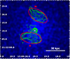 |
Fig. 8. 0.5−7 keV Chandra image of Abell 2009 convolved with a Gaussian function of a 2 pixel radius. The green contours identify the radio emission at 1.5 GHz. The rms noise is σrms = 19 μJy/beam. The contour levels start from 3σ and increase by a factor 2, while the beam size is 1.2″ × 1.1″. The red regions correspond to the north and south regions used to describe the size of the radio lobes (N and S). The white cross corresponds to the position of the BCG. |
Morphology of the BCG radio lobes of Abell 2009.
In order to derive the mechanical AGN power, Pcav = 4 pV/tcav, we first calculate the pV work done by the AGN to inflate the lobe. We consider the ICM pressure within the first annulus of the deprojected spectral analysis (see Table 6), which encompasses both radio lobes, measuring a mechanical energy of about 4 pV = 3 × 1059 erg for each lobe. The radio lobes seem to be detected at an early evolutionary state since they are relatively close to the AGN, at about 15−20 kpc from the center. Thus, we compute the dynamical age of the radio lobes using the sound crossing time, tsc. This timescale assumes that the bubbles are rising through the hot gas atmosphere at the ICM sound speed, defined as:

The sound crossing time of the lobes is thus: tcav = d/cs, where d is the distance of the lobe from the BCG (reported in Table 9). The sound speed in the first annulus is cs = 936 ± 72 km s−1 and the corresponding lobes ages are approximately 26.8 Myr (N) and 13.5 Myr (S). The estimated mechanical AGN power values are thus ∼3.8 × 1044 erg s−1 (N) and 7.5 × 1044 erg s−1 (S). These results are reported in Table 10. The power of the N and S lobes is summed to obtain the total cavity power:

Energetics of the BCG radio lobes of Abell 2009.
where the error is calculated as the dispersion at 1σ from the mean value.
We are aware that these estimates are relatively uncertain and that the real uncertainties are probably dominated by systematics, as the lobes could be older than measured with the sound crossing time. Considering other methods to derive the age of cavities and bubbles, the discrepancy could be up to a factor of two (e.g., Bîrzan et al. 2004; Ubertosi et al. 2021). Projection effects constitute another important source of uncertainty. Additionally, the assumption of the radio lobes being representative tracers of cavities adds further uncertainties. On the one hand, any X-ray cavity could be smaller than the lobes at 1.5 GHz, thus leading to an overestimate of their volume (and thus the energy). However, the radio lobes may be larger at lower frequencies (≈100 s MHz), where radiative losses of relativistic electrons are less effective in dimming the synchrotron emission than at 1.5 GHz (see the example of MS 0735.6+7421; e.g., Biava et al. 2021). These two opposite effects prevent us from deriving an accurate estimate of the size of the cavities from the radio tracer. All in all, we consider that systematic uncertainties on energy and age of the radio lobes may be up to a factor of two, and those on the mechanical power may be up to a factor of four. The value of the X-ray luminosity inside the cooling region, obtained in Sect. 3.3.4, is Lcool = (4.4 ± 0.1) × 1044 erg s−1. This measure is a factor of two lower than the mechanical power estimated from the central radio galaxy’s lobes, suggesting that the cooling luminosity (Lcool) can be balanced by the mechanical power (Pcav). Even if the cavities were assumed to be half as large and twice as old – reducing the mechanical power by a factor of four – the resulting power would still be approximately 3 × 1044 erg s−1, remaining comparable to the cooling luminosity. This indicates that, even under conservative assumptions, AGN mechanical feedback is likely sufficient to counterbalance radiative losses in Abell 2009’s core region.
4.2. Clusters sample properties
Abell 2009 has been extracted from a ROSAT BCS subsample in which 18 clusters with X-ray fluxes greater than 4.4 × 10⁻¹² erg cm−2 s−1 (Ebeling et al. 1998) and Hα luminosities greater than 1040 erg s−1 (Crawford et al. 1999) were selected (see Table 1). To obtain a general perspective on the AGN feedback process, it is interesting to investigate how the ICM properties may vary with the central AGN ones in the objects of this subsample. We thus examine both the AGN properties, such as cavity power (Pcav), cavity energy (Ecav) and cavity age (tcav), as well as the properties of the ICM, in particular the cooling luminosity (Lcool). For most objects, these measurements are available from the literature (see references in Table 1)4. Given the nonhomogeneous analysis of the subsample, we assume a conservative 50% relative uncertainty. Moreover, we also consider the cooling time at 12 kpc from the center, reported by Rafferty et al. (2008) for 9/18 of the clusters in our selection, along with the associated uncertainty, and we derive a similar estimate for Abell 2009 (from this work), ZwCl 235 (from Ubertosi et al. 2023c), Abell 1668 (from Pasini et al. 2021), and Abell 2495 (from Rosignoli et al. 2024). Such a small radius of 12 kpc should capture the most rapidly cooling part of the ICM. We note that, for Abell 2009 and Abell 2495, the innermost radial bin of the thermodynamic profile (and thus the smallest resolution element) is at a radius of 16.8 kpc and 23.6 kpc, respectively. Therefore, there may be slight variations with respect to the actual cooling time at 12 kpc. These measures are reported in Table 1.
We caution that the following discussion aims at exploring general trends between relevant quantities for our selection of systems and it is not intended to represent a statistical assessment of scaling relations for galaxy clusters in general.
4.2.1. Cavity power versus cooling luminosity
The cavity power, Pcav, representing the mechanical energy injected into the hot gas by the AGN outburst, can then be directly compared to the gas luminosity within the cooling radius, Lcool, representing the radiative gas losses due to cooling. As we show in Fig. 9 (upper left panel), cavity power scales in proportion to the cooling X-ray luminosity, albeit with considerable scatter. This is a confirmation of the well-known relation between heating power and cooling losses found in several other works5 (e.g., Bîrzan et al. 2004; Rafferty et al. 2006; Fabian 2012).
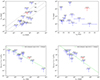 |
Fig. 9. Correlation between ICM and AGN properties for the galaxy clusters reported in Table 1. Upper left panel: Cavities power as function of the X-ray luminosity inside the cooling radius of each galaxy cluster. The diagonal lines indicate Pcav = Lcool assuming different values for the adiabatic index γ. All the uncertainties are set to 50% for consistency. Upper right panel: Cavity power as a function of the cooling time at 12 kpc from the clusters center. All the uncertainties on the cavity power are set to 50%, while the errors associated with the cooling time are reported in Table 1. Lower left panel: Number of outbursts required to counterbalance the radiative losses of the cooling gas as a function of the cavity energy. The green line represents the best-fit line derived using the BCES orthogonal regression method. All the uncertainties on the cavity energy and cooling luminosity are set to 50%, while the errors associated with the cooling time are reported in Table 1. Lower right panel: Number of outbursts required to counterbalance the radiative losses of the cooling gas as a function of the cavity power. The green line represents the best-fit line derived using the BCES orthogonal regression method. All the uncertainties on the cavity energy, cavity power and cooling luminosity are set to 50%, while the errors associated with the cooling time are reported in Table 1. |
We note that Abell 2204 has a significantly higher value for the cavities power with respect to the other galaxy clusters of the sample, lying well above the linear relation Pcav = Lcool. This is mainly driven by the presence, according to Sanders et al. (2009), of a giant cavity with a very large mechanical power in the cluster, which dominates the total energy budget. Similarly, Abell 2390 also lies above the same line, though with a smaller offset. This behavior indicates that the energy provided by its outburst exceeds the amount needed to counteract cooling.
Even though our selection of cool cores does not constitute a complete sample, it is likely representative of systems where AGN feedback is ongoing and as such, we expect a similar Pcav − Lcool scaling to hold in other similar systems. In this respect, we note that a linear scaling relation between these quantities was confirmed to exist even in complete samples of galaxy clusters (see the study of Bîrzan et al. 2012).
4.2.2. Cavity power versus cooling time
We also examine the possible correlation between the power of the AGN’s outburst and the central gas cooling time. From the point of view of the feeding side of the self-regulated loop, a short gas cooling time is able to supply the central AGN with a strong inflow of cool gas, possibly leading to more powerful mechanical outbursts, so an anticorrelation may be expected (Dunn & Fabian 2006). On the other hand, from the point of view of the feedback side of the self-regulated loop, long cooling times could be the result of the heating effect of a highly powerful outburst on the surrounding gas, so a direct correlation may be expected. However, as we show in Fig. 9 (upper right panel), no significant correlation is visible. For example, outbursts with power ∼1043 erg s−1 can be found in X-ray atmospheres whose central cooling time can vary by an order of magnitude, between about 0.2 and 2 Gyr. More insights on the Pcav − tcool relation can be derived by considering that the two quantities reflect processes with different timescales; the cavities age (≈tens of Myr) is typically shorter than the time needed by the gas to cool (≈1 Gyr). It is also evident that despite the highest energetic AGN outbursts, the gas cooling time remains below ∼1.5 Gyr in the central regions. In this respect, McNamara & Nulsen (2012) pointed out that the most powerful AGN outbursts do not significantly raise the central gas temperature or lower the central gas density. On the other hand, they increase the central gas entropy through a gentle heating process.
4.2.3. Outburst occurrence versus outburst energy and power
We investigate the outburst occurrence by considering the quantity Lcool × tcool/Ecav, that represents the number of AGN outbursts of energy Ecav required to counterbalance the radiative losses of the cooling gas (assuming a duty cycle = 1). As it can be seen in Fig. 9 (lower left and right panels), the Lcool × tcool/Ecav quantity is plotted against the cavity energy, Ecav, and the cavity power, Pcav, respectively. In both cases, the data are fitted using the BCES orthogonal regression method (Akritas & Bershady 1996), revealing two linear anti-correlations. For the cavity energy plot, the slope of the best-fit line is −0.78 ± 0.12, with Pearson and Spearman correlation coefficients of −0.92 and −0.79, respectively. Similarly, for the cavity power plot, the slope is −1.06 ± 0.26, and the corresponding Pearson and Spearman coefficients are −0.88 and −0.78. In general, these plots indicate that more energetic outbursts and more powerful outbursts require a lower frequency in order to counterbalance the radiative losses due to cooling.
This is clearly exemplified by Abell 2390, that while lying well above the 4 pV line in Fig. 9 (top left panel), also requires about 0.1 such outbursts per cooling time to counterbalance the radiative losses of its hot gas halo (Fig. 9, lower panels). As explained in Bîrzan et al. (2004), clusters that require less than 4 pV will be reasonably supplied with energy in the cavities to balance cooling, while for clusters requiring more than 16 pV per cavity, it is more difficult to balance cooling, if no other forms of heating are present. Indeed, as it can be observed in Fig. 9 (lower panels), clusters with a higher Pcav value require a smaller amount of AGN outburst to balance the cooling.
A similar result is obtained in the study of Vantyghem et al. (2014), where the cavity heating time was defined as the amount of time that the cavity energy is able to offset radiative losses, which is Ecav/Lcool. Comparing the cavity heating time with the outburst interval of 13 different systems, the authors derived that more energetic outbursts offset cooling with longer outburst intervals. Moreover, the outburst interval is often shorter than the correspondent cavity heating time, suggesting that heating continually compensates for radiative cooling through the cluster’s lifetime.
To conclude, we have investigated the relationship between AGN heating and ICM cooling properties in a collection of 18 clusters, adding our results on Abell 2009 to the literature work on the remaining clusters, performed using different methods. However, we note that a homogeneous analysis of larger samples would be necessary to better investigate and confirm the relationships discussed in this work.
5. Conclusions
In this work, we presented Chandra and 1.5 GHz VLA observations of the galaxy cluster Abell 2009 by performing in particular a detailed X-ray analysis of its ICM for the first time.
The main results we obtained are briefly summarized below:
-
The BCG has a total 1.5 GHz flux density of 23 ± 1 mJy, with 5.8 ± 0.3 mJy coming from the central bright core. Its extended radio lobes present a symmetric butterfly-shaped morphology. The radio galaxy in the N direction has a total flux density of 41 ± 1.6 mJy, including the core emission, and is a cluster member of Abell 2009. Located approximately 130 kpc from the center of Abell 2009, this radio source may be interacting with the cluster’s ICM.
-
The global properties of the ICM of Abell 2009 are kT = 6.41 ± 0.17 keV and Z = 0.59 ± 0.07 Z⊙. The morphological analysis confirmed the cool-core nature of Abell 2009, since its surface brightness profile is peaked at center and is best-fitted with a double β model. From the spectral analysis, the cooling radius results to be rcool = 87.5 ± 15.7 kpc, within which the cooling time is lower than 7.7 Gyr. The X-ray luminosity inside the cooling region is Lcool = (4.4 ± 0.1)×1044 erg s−1.
-
As found for several other cool-core clusters, we confirm the mismatch in Abell 2009 between the theoretical, global mass inflow rate (Ṁglob = (316 ± 16) M⊙/yr) expected in the standard cooling flow model and the spectral mass inflow rate (Ṁspec ≤ 19.4 M⊙/yr). This discrepancy is consistent with the presence of a heating mechanism that can reduce the efficiency of the cooling process in the central region of the cluster.
-
No clear depressions are detected in the X-ray image, possibly due to the relatively short exposure. Guided by the radio images under the assumption that any underlying X-ray cavity is traced by radio bubbles, we measure the properties of possible cavities corresponding to the radio lobes of the BCG. The N lobe and S lobe have ages of ≈27 Myr and ≈14 Myr, respectively. The lobes total power is ≈1045 erg s−1. Comparing this value with the X-ray luminosity inside the cooling region, it can be inferred that the mechanical power associated to the activity of the central AGN is able to counterbalance the cooling process of the ICM.
-
Finally, we briefly investigate the general properties of the parent sample of galaxy clusters with high X-ray flux and high Hα luminosity from which Abell 2009 was selected. We discuss the lack of correlation between cavity power and cooling time as a result of the feedback from cluster-central AGN being gentle and not disruptive. Moreover, we find indications that more energetic and powerful outbursts require a lower frequency, compared to less energetic ones, to balance the radiative losses resulting from gas cooling.
In some cases, the properties of the identified cavities were not reported in literature, while in other cases no cavities were detected in the existing exposures (see caption of Table 1). When cavities are absent, cooling may still be balanced through alternative mechanisms (as discussed in e.g., Mathews et al. 2006; McNamara & Nulsen 2007). However, these non-detections should not significantly impact the correlations discussed in this work, as cavities are identified in 85% of the cases within our selection.
We note that the definition of cooling luminosity of Bîrzan et al. (2004) and Rafferty et al. (2006) differs from later studies, including ours. Specifically, these early works investigated the relation between Pcav and LX − Lspec, X, where LX and Lspec, X are the luminosities inside the cooling region of the apec and mkcflow components, respectively, whereas subsequent studies have focused on Pcav versus LX alone (e.g., Bîrzan et al. 2012; Hlavacek-Larrondo et al. 2013; Ubertosi et al. 2023c; Ruppin et al. 2023). The reason for using LX alone as the estimate of the cooling luminosity is mainly due to the limited spectral resolution of Chandra CCDs, which prevents accurate measurements of cooling rates in large spatial extraction regions, and to the fact that early estimates indicate that Lspec, X is a small fraction (∼10% or less) of LX (e.g., Sanders et al. 2008). In any case, we note that this potential offset given by neglecting Lspec, X is absorbed within the conservatively large systematic uncertainty (ΔLX/LX = 50%) assumed in our analysis.
Acknowledgments
This paper and related research have been conducted during and with the support of the Italian national inter-university PhD programme in Space Science and Technology – University of Trento/IUSS Pavia. FU and MG acknowledge the financial contribution from contract PRIN 2022 – CUP J53D23001610006. The authors thank the anonymous reviewer for providing useful feedback on this manuscript.
References
- Ahumada, R., Allende Prieto, C., Almeida, A., et al. 2020, ApJS, 249, 3 [NASA ADS] [CrossRef] [Google Scholar]
- Akritas, M. G., & Bershady, M. A. 1996, ApJ, 470, 706 [Google Scholar]
- Asplund, M., Grevesse, N., Sauval, A. J., & Scott, P. 2009, ARA&A, 47, 481 [NASA ADS] [CrossRef] [Google Scholar]
- Bahcall, N. A. 1996, Clusters and Superclusters of Galaxies (Princeton University Observatory) [Google Scholar]
- Banfield, J. K., Wong, O. I., Willett, K. W., et al. 2015, MNRAS, 453, 2327 [CrossRef] [Google Scholar]
- Best, P. N., & Heckman, T. M. 2012, MNRAS, 421, 1569 [NASA ADS] [CrossRef] [Google Scholar]
- Best, P. N., von der Linden, A., Kauffmann, G., Heckman, T. M., & Kaiser, C. R. 2007, MNRAS, 379, 894 [Google Scholar]
- Biava, N., Brienza, M., Bonafede, A., et al. 2021, A&A, 650, A170 [NASA ADS] [CrossRef] [EDP Sciences] [Google Scholar]
- Bîrzan, L., Rafferty, D. A., McNamara, B. R., Wise, M. W., & Nulsen, P. E. J. 2004, ApJ, 607, 800 [Google Scholar]
- Bîrzan, L., McNamara, B. R., Nulsen, P. E. J., Carilli, C. L., & Wise, M. W. 2008, ApJ, 686, 859 [Google Scholar]
- Bîrzan, L., Rafferty, D. A., Nulsen, P. E. J., et al. 2012, MNRAS, 427, 3468 [Google Scholar]
- Blanton, E. L., Sarazin, C. L., McNamara, B. R., & Wise, M. W. 2001, ApJ, 558, L15 [NASA ADS] [CrossRef] [Google Scholar]
- Blanton, E. L., Randall, S. W., Clarke, T. E., et al. 2011, ApJ, 737, 99 [Google Scholar]
- Brighenti, F., & Mathews, W. G. 2006, ApJ, 643, 120 [NASA ADS] [Google Scholar]
- Burns, J. O. 1990, AJ, 99, 14 [NASA ADS] [CrossRef] [Google Scholar]
- CASA Team (Bean, B., et al.) 2022, PASP, 134, 114501 [NASA ADS] [CrossRef] [Google Scholar]
- Cavaliere, A., & Fusco-Femiano, R. 1978, A&A, 70, 677 [NASA ADS] [Google Scholar]
- Condon, J. J., Cotton, W. D., Greisen, E. W., et al. 1998, AJ, 115, 1693 [Google Scholar]
- Crawford, C. S., Allen, S. W., Ebeling, H., Edge, A. C., & Fabian, A. C. 1999, MNRAS, 306, 857 [CrossRef] [Google Scholar]
- David, L. P., Nulsen, P. E. J., McNamara, B. R., et al. 2001, ApJ, 557, 546 [CrossRef] [Google Scholar]
- Domainko, W., Gitti, M., Schindler, S., & Kapferer, W. 2004, A&A, 425, L21 [NASA ADS] [CrossRef] [EDP Sciences] [Google Scholar]
- Donahue, M., & Voit, G. M. 2022, Phys. Rep., 973, 1 [NASA ADS] [CrossRef] [Google Scholar]
- Dunn, R. J. H., & Fabian, A. C. 2006, MNRAS, 373, 959 [Google Scholar]
- Ebeling, H., Edge, A. C., Bohringer, H., et al. 1998, MNRAS, 301, 881 [Google Scholar]
- Edge, A. C. 2001, MNRAS, 328, 762 [NASA ADS] [CrossRef] [Google Scholar]
- Ettori, S. 2000, MNRAS, 318, 1041 [Google Scholar]
- Ettori, S., Gastaldello, F., Gitti, M., et al. 2013, A&A, 555, A93 [NASA ADS] [CrossRef] [EDP Sciences] [Google Scholar]
- Fabian, A. C. 1994, ARA&A, 32, 277 [Google Scholar]
- Fabian, A. C. 2012, ARA&A, 50, 455 [Google Scholar]
- Fabian, A. C., Mushotzky, R. F., Nulsen, P. E. J., & Peterson, J. R. 2001, MNRAS, 321, L20 [NASA ADS] [CrossRef] [Google Scholar]
- Fabian, A. C., Sanders, J. S., Allen, S. W., et al. 2003, MNRAS, 344, L43 [NASA ADS] [CrossRef] [Google Scholar]
- Fabian, A. C., Ferland, G. J., Sanders, J. S., et al. 2022, MNRAS, 515, 3336 [NASA ADS] [CrossRef] [Google Scholar]
- Fanaroff, B. L., & Riley, J. M. 1974, MNRAS, 167, 31P [Google Scholar]
- Ferland, G. J., Korista, K. T., Verner, D. A., et al. 1998, PASP, 110, 761 [Google Scholar]
- Fruscione, A., McDowell, J. C., Allen, G. E., et al. 2006, SPIE Conf. Ser., 6270, 62701V [Google Scholar]
- Gaia Collaboration (Brown, A. G. A., et al.) 2018, A&A, 616, A1 [NASA ADS] [CrossRef] [EDP Sciences] [Google Scholar]
- Gaspari, M., Melioli, C., Brighenti, F., & D’Ercole, A. 2011, MNRAS, 411, 349 [Google Scholar]
- Gaspari, M., Brighenti, F., & Temi, P. 2012, MNRAS, 424, 190 [NASA ADS] [CrossRef] [Google Scholar]
- Gaspari, M., Tombesi, F., & Cappi, M. 2020, Nat. Astron., 4, 10 [Google Scholar]
- Gitti, M., Brighenti, F., & McNamara, B. R. 2012, Adv. Astron., 2012, 1 [CrossRef] [Google Scholar]
- Hamer, S. L., Edge, A. C., Swinbank, A. M., et al. 2016, MNRAS, 460, 1758 [Google Scholar]
- HI4PI Collaboration (Ben Bekhti, N., et al.) 2016, A&A, 594, A116 [NASA ADS] [CrossRef] [EDP Sciences] [Google Scholar]
- Hlavacek-Larrondo, J., Allen, S. W., Taylor, G. B., et al. 2013, ApJ, 777, 163 [Google Scholar]
- Hogan, M. T., Edge, A. C., Hlavacek-Larrondo, J., et al. 2015, MNRAS, 453, 1201 [NASA ADS] [CrossRef] [Google Scholar]
- Kimball, A. E., & Ivezić, Ž. 2008, AJ, 136, 684 [Google Scholar]
- Ledlow, M. J., & Owen, F. N. 1996, AJ, 112, 9 [Google Scholar]
- Lewis, A. D., Buote, D. A., & Stocke, J. T. 2003, ApJ, 586, 135 [NASA ADS] [Google Scholar]
- Li, Y., Bryan, G. L., Ruszkowski, M., et al. 2015, ApJ, 811, 73 [Google Scholar]
- Markevitch, M., & Vikhlinin, A. 2007, Phys. Rep., 443, 1 [Google Scholar]
- Markevitch, M., Vikhlinin, A., & Mazzotta, P. 2001, ApJ, 562, L153 [NASA ADS] [CrossRef] [Google Scholar]
- Mathews, W. G., & Brighenti, F. 2003, ApJ, 590, L5 [NASA ADS] [Google Scholar]
- Mathews, W. G., Faltenbacher, A., & Brighenti, F. 2006, ApJ, 638, 659 [CrossRef] [Google Scholar]
- McDonald, M., Veilleux, S., Rupke, D. S. N., & Mushotzky, R. 2010, ApJ, 721, 1262 [Google Scholar]
- McNamara, B., & Nulsen, P. 2007, ARA&A, 45, 117 [NASA ADS] [CrossRef] [Google Scholar]
- McNamara, B. R., & Nulsen, P. E. J. 2012, New J. Phys., 14, 055023 [NASA ADS] [CrossRef] [Google Scholar]
- McNamara, B. R., Wise, M. W., & Murray, S. S. 2004, ApJ, 601, 173 [NASA ADS] [CrossRef] [Google Scholar]
- McNamara, B. R., Rafferty, D. A., Bîrzan, L., et al. 2006, ApJ, 648, 164 [NASA ADS] [CrossRef] [Google Scholar]
- Mohr, J. J., Mathiesen, B., & Evrard, A. E. 1999, ApJ, 517, 627 [Google Scholar]
- Morris, R., & Fabian, A. C. 2003, MNRAS, 338, 824 [NASA ADS] [CrossRef] [Google Scholar]
- Mushotzky, R. F., & Szymkowiak, A. E. 1988, NATO Advanced Study Institute (ASI) Series C, 229, 53 [Google Scholar]
- Nulsen, P. E. J., Li, Z., Forman, W. R., et al. 2013, ApJ, 775, 117 [NASA ADS] [CrossRef] [Google Scholar]
- Olivares, V., Salome, P., Combes, F., et al. 2019, A&A, 631, A22 [NASA ADS] [CrossRef] [EDP Sciences] [Google Scholar]
- Olivares, V., Su, Y., Nulsen, P., et al. 2022, MNRAS, 516, L101 [NASA ADS] [CrossRef] [Google Scholar]
- Pandge, M. B., Vagshette, N. D., Sonkamble, S. S., & Patil, M. K. 2013, Astrophys. Space Sci., 345, 183 [Google Scholar]
- Pasini, T., Gitti, M., Brighenti, F., et al. 2019, ApJ, 885, 111 [NASA ADS] [CrossRef] [Google Scholar]
- Pasini, T., Gitti, M., Brighenti, F., et al. 2021, ApJ, 911, 66 [NASA ADS] [CrossRef] [Google Scholar]
- Peterson, J., & Fabian, A. 2006, Phys. Rep., 427, 1 [NASA ADS] [CrossRef] [Google Scholar]
- Quillen, A. C., Zufelt, N., Park, J., et al. 2008, ApJS, 176, 39 [NASA ADS] [CrossRef] [Google Scholar]
- Rafferty, D. A., McNamara, B. R., Nulsen, P. E. J., & Wise, M. W. 2006, ApJ, 652, 216 [NASA ADS] [CrossRef] [Google Scholar]
- Rafferty, D. A., McNamara, B. R., & Nulsen, P. E. J. 2008, ApJ, 687, 899 [NASA ADS] [CrossRef] [Google Scholar]
- Rosignoli, L., Ubertosi, F., Gitti, M., et al. 2024, ApJ, 963, 8 [Google Scholar]
- Rossetti, M., & Molendi, S. 2010, A&A, 510, A83 [NASA ADS] [CrossRef] [EDP Sciences] [Google Scholar]
- Ruppin, F., McDonald, M., Hlavacek-Larrondo, J., et al. 2023, ApJ, 948, 49 [NASA ADS] [CrossRef] [Google Scholar]
- Russell, H. R., McNamara, B. R., Fabian, A. C., et al. 2017, MNRAS, 472, 4024 [NASA ADS] [CrossRef] [Google Scholar]
- Sanders, J. S., Fabian, A. C., Allen, S. W., et al. 2008, MNRAS, 385, 1186 [NASA ADS] [CrossRef] [Google Scholar]
- Sanders, J. S., Fabian, A. C., & Taylor, G. B. 2009, MNRAS, 393, 71 [CrossRef] [Google Scholar]
- Sarazin, C. L. 1986, Rev. Mod. Phys., 58, 1 [Google Scholar]
- Seth, R., O’Sullivan, E., Sebastian, B., et al. 2022, MNRAS, 513, 3273 [NASA ADS] [CrossRef] [Google Scholar]
- Sonkamble, S. S., Vagshette, N. D., Pawar, P. K., & Patil, M. K. 2015, Astrophys. Space Sci., 359, 21 [Google Scholar]
- Sternberg, A., & Soker, N. 2008, MNRAS, 384, 1327 [CrossRef] [Google Scholar]
- Sun, M., Jones, C., Murray, S. S., et al. 2003, ApJ, 587, 619 [NASA ADS] [CrossRef] [Google Scholar]
- Sutherland, R. S., & Dopita, M. A. 1993, ApJS, 88, 253 [Google Scholar]
- Timmerman, R., van Weeren, R. J., Botteon, A., et al. 2022, A&A, 668, A65 [NASA ADS] [CrossRef] [EDP Sciences] [Google Scholar]
- Ubertosi, F., Gitti, M., Brighenti, F., et al. 2021, ApJ, 923, L25 [NASA ADS] [CrossRef] [Google Scholar]
- Ubertosi, F., Gitti, M., Brighenti, F., et al. 2023a, ApJ, 944, 216 [NASA ADS] [CrossRef] [Google Scholar]
- Ubertosi, F., Gitti, M., Brighenti, F., et al. 2023b, A&A, 673, A52 [NASA ADS] [CrossRef] [EDP Sciences] [Google Scholar]
- Ubertosi, F., Gitti, M., & Brighenti, F. 2023c, A&A, 670, A23 [NASA ADS] [CrossRef] [EDP Sciences] [Google Scholar]
- Vantyghem, A. N., McNamara, B. R., Russell, H. R., et al. 2014, MNRAS, 442, 3192 [Google Scholar]
- Vantyghem, A. N., McNamara, B. R., Russell, H. R., et al. 2016, ApJ, 832, 148 [Google Scholar]
- Voigt, L. M., Schmidt, R. W., Fabian, A. C., Allen, S. W., & Johnstone, R. M. 2002, MNRAS, 335, L7 [NASA ADS] [CrossRef] [Google Scholar]
- Wong, K.-W., Sarazin, C. L., Blanton, E. L., & Reiprich, T. H. 2008, ApJ, 682, 155 [NASA ADS] [CrossRef] [Google Scholar]
- ZuHone, J. A., Markevitch, M., & Johnson, R. E. 2010, ApJ, 717, 908 [Google Scholar]
Appendix A: Additional table
In this Section, we report the table with the best-fit results of the projected spectral analysis (see Subsec. 3.3.2).
Best-fit results of the projected radial analysis of Abell 2009.
All Tables
Selection of high X-ray flux and high Hα luminosity galaxy clusters from the BCS sample.
All Figures
|
Fig. 1. Multiwavelength view of Abell 2009. Left panel: In this image, the radio emission at 1.5 GHz observed with the JVLA telescope and the X-ray emission detected by the Chandra telescope are shown in red and blue, respectively. Both emissions are overlaid on an optical image from the DESI survey for a comprehensive view of the system. Upper right panel: 1.5 GHz JVLA radio image zoomed on the BCG, at a resolution of 1.2″ × 1.1″. The rms value is σrms = 19 μJy/beam. Magenta contour levels are taken at 3, 6, 12, 24 × σrms. Lower right panel: 1.5 GHz JVLA radio image zoomed on the northern radio galaxy, at a resolution of 1.2″ × 1.1″. The rms value is σrms = 19 μJy/beam. Magenta contour levels are taken at 3, 6, 12, 24 × σrms. |
| In the text | |
|
Fig. 2. 0.5−7 keV Chandra image of the galaxy cluster Abell 2009, convolved with a Gaussian function of a 2 pixel radius. |
| In the text | |
|
Fig. 3. 0.5−7 keV surface brightness profile of Abell 2009 fitted with a single β model. The lower subplot represents the residuals in σ units. |
| In the text | |
|
Fig. 4. Left panel: 0.5−7 keV surface brightness profile of Abell 2009 fitted with a double β model where the values of β are unlinked (see Table 3). The orange line represents the total model, while the red and green lines correspond to the two components of the model. The lower subplot represents the residuals in σ units. Right panel: 0.5−7 keV surface brightness profile of Abell 2009 fitted with a double β model where the values of β are linked (see Table 3). The orange line represents the total model, while the red and green lines correspond to the two components of the model. The lower subplot represents the residuals in σ units. |
| In the text | |
|
Fig. 5. Residual image of the best-fit double β model convolved with a Gaussian function of a 5 pixel radius. The green contours identify the radio emission at 1.5 GHz. The rms noise is σrms = 19 μJy/beam. The contour levels start from 3σ and increase by a factor 2, while the beam size is 1.2″ × 1.1″. The black cross corresponds to the position of the BCG. |
| In the text | |
|
Fig. 6. Projected (blue) and deprojected (red) radial temperature profiles of Abell 2009. The temperature measurements are reported in Tables A.1 and 6. |
| In the text | |
|
Fig. 7. Radial profiles of thermodynamic properties of Abell 2009. First panel: Deprojected electron density profile of Abell 2009. Second panel: Deprojected pressure profile of Abell 2009. Third panel: Deprojected entropy profile of Abell 2009. Forth panel: Cooling time profile fitted with a polynomial fit (yellow line) showing the interception with the red horizontal line corresponding to a 7.7 Gyr cooling time and the black vertical line corresponding to the cooling radius value (87.5 kpc). |
| In the text | |
|
Fig. 8. 0.5−7 keV Chandra image of Abell 2009 convolved with a Gaussian function of a 2 pixel radius. The green contours identify the radio emission at 1.5 GHz. The rms noise is σrms = 19 μJy/beam. The contour levels start from 3σ and increase by a factor 2, while the beam size is 1.2″ × 1.1″. The red regions correspond to the north and south regions used to describe the size of the radio lobes (N and S). The white cross corresponds to the position of the BCG. |
| In the text | |
|
Fig. 9. Correlation between ICM and AGN properties for the galaxy clusters reported in Table 1. Upper left panel: Cavities power as function of the X-ray luminosity inside the cooling radius of each galaxy cluster. The diagonal lines indicate Pcav = Lcool assuming different values for the adiabatic index γ. All the uncertainties are set to 50% for consistency. Upper right panel: Cavity power as a function of the cooling time at 12 kpc from the clusters center. All the uncertainties on the cavity power are set to 50%, while the errors associated with the cooling time are reported in Table 1. Lower left panel: Number of outbursts required to counterbalance the radiative losses of the cooling gas as a function of the cavity energy. The green line represents the best-fit line derived using the BCES orthogonal regression method. All the uncertainties on the cavity energy and cooling luminosity are set to 50%, while the errors associated with the cooling time are reported in Table 1. Lower right panel: Number of outbursts required to counterbalance the radiative losses of the cooling gas as a function of the cavity power. The green line represents the best-fit line derived using the BCES orthogonal regression method. All the uncertainties on the cavity energy, cavity power and cooling luminosity are set to 50%, while the errors associated with the cooling time are reported in Table 1. |
| In the text | |
Current usage metrics show cumulative count of Article Views (full-text article views including HTML views, PDF and ePub downloads, according to the available data) and Abstracts Views on Vision4Press platform.
Data correspond to usage on the plateform after 2015. The current usage metrics is available 48-96 hours after online publication and is updated daily on week days.
Initial download of the metrics may take a while.