| Issue |
A&A
Volume 695, March 2025
|
|
|---|---|---|
| Article Number | A7 | |
| Number of page(s) | 8 | |
| Section | Extragalactic astronomy | |
| DOI | https://doi.org/10.1051/0004-6361/202452979 | |
| Published online | 26 February 2025 | |
The evolution of extragalactic peaked-spectrum sources down to 54 megahertz
1
Leiden Observatory, Leiden University, PO Box 9513 2300 RA Leiden, The Netherlands
2
NSF NOIRLab, Gemini Observatory, 670 N A’ohoku Place Hilo, HI 96720, USA
3
Centre for Astrophysics Research, University of Hertfordshire, College Lane, Hatfield AL10 9AB, UK
4
CSIRO Space and Astronomy, ATNF, PO Box 1130 Bentley, WA 6102, Australia
5
INAF – Istituto di Radioastronomia, Via P. Gobetti 101, 40129 Bologna, Italy
⋆ Corresponding author; This email address is being protected from spambots. You need JavaScript enabled to view it.
Received:
13
November
2024
Accepted:
28
January
2025
Abstract
Peaked-spectrum sources, known for their distinct peaked radio spectra, are a type of radio-loud active galactic nuclei. One subtype, megahertz-peaked-spectrum (MPS) sources, which exhibit a spectral peak at a frequency of a hundred megahertz, have emerged as a potential tool for identifying high-redshift candidates. However, the potential evolutionary link between the fraction of these sources and their redshifts remains unclear and requires further investigation. The recent, high-sensitivity Low Frequency Array (LOFAR) surveys enable statistical studies of these objects down to ultra-low frequencies (< 150 MHz). In this study we first used the multi-radio data to investigate the evolution of spectral index with redshift for 1187 quasars from the 16th SDSS quasar catalog. For each quasar, we analyzed available data from the LOFAR Low Band Antenna at 54 MHz, the High Band Antenna at 144 MHz, and the Very Large Array Faint Images of the Radio Sky at Twenty centimeters at 1.4 GHz. We measured the spectral index (α54144 and α1441400) and find no significant change in their median values with redshift. Extended sources have steeper spectral indices than compact sources, which is consistent with previous findings. Based on the spectral index information, we identified MPS sources using the criteria α54144 > = 0.1 and α1441400 < 0, and analyzed their properties. We find that the fraction of MPS sources is constant with the redshift (0.1 − 4.8), bolometric luminosity (1044 − 1048 erg/s), and supermassive black hole mass (107 − 1010.5 M⊙), which suggests that MPS sources have relatively stable physical conditions or formation mechanisms across various evolutionary stages and environments.
Key words: Galaxy: general / galaxies: active / galaxies: general / galaxies: high-redshift / galaxies: nuclei
© The Authors 2025
 Open Access article, published by EDP Sciences, under the terms of the Creative Commons Attribution License (https://creativecommons.org/licenses/by/4.0), which permits unrestricted use, distribution, and reproduction in any medium, provided the original work is properly cited.
This article is published in open access under the Subscribe to Open model. This email address is being protected from spambots. You need JavaScript enabled to view it. to support open access publication.
1. Introduction
Quasars are among the most luminous and energetic objects in the Universe (e.g., Schmidt 1963; Shields 1999). These active galactic nuclei (AGNs) are powered by supermassive black holes (SMBHs) at the center of galaxies through the accretion of large amounts of material (e.g., Rees 1984; Kormendy & Richstone 1995). Their extreme luminosities allow us to detect them at great distances, thereby enabling the study of the high-redshift Universe and insights into various subsets of AGNs, including the peaked-spectrum (PS) sources (e.g., Fan et al. 2006; Coppejans et al. 2015; Yang et al. 2020; Wang et al. 2021).
Peaked-spectrum (PS) sources are characterized by their peaked radio spectra. Based on their peak frequency (νo), they are divided into high-frequency-peaked (HFP) sources that peak above 5 GHz, gigahertz-peaked-spectrum (GPS) sources that peak at 1–5 GHz, compact steep spectrum (CSS) sources that peak below 500 MHz, and megahertz-peaked-spectrum (MPS) sources that peak below 1 GHz in the observed frame (Fanti et al. 1990; O’Dea et al. 1991; Dallacasa et al. 2000; Coppejans et al. 2016; Callingham et al. 2017; Ballieux et al. 2024). These sources exhibit small linear sizes: HFP and GPS sources are smaller than 1 kpc, while CSS sources range from 1-20 kpc (O’Dea 1998). Previous work also found larger sources tend to have lower peak frequencies (O’Dea & Baum 1997; Snellen et al. 2000).
Despite extensive research, the reason for the turnover in their radio spectra remains unclear. Two models – the “youth” and “frustration” models – have been proposed to explain these turnovers. The youth model suggests that these sources follow an evolutionary sequence, with HFP sources gradually maturing into GPS sources, then CSS sources, and ultimately evolving into Fanaroff–Riley (FR) I and FR II radio galaxies (Murgia et al. 2002; Kunert-Bajraszewska et al. 2010). In contrast, the frustration model posits that these sources are not young and attributes their small size to confinement by the surrounding dense, hot nuclear plasma, which slows the expansion of the sources (van Breugel et al. 1984). It is also possible that both mechanisms contribute to the turnover of PS sources (An & Baan 2012; Callingham et al. 2017), meaning that both synchrotron self-absorption (suggested by the youth model) and free-free absorption (suggested by the frustration model) may contribute to these spectral turnovers (Bicknell et al. 1997; Marr et al. 2014; Keim et al. 2019). Typically, the youth model predicts a spectral index near 2.5, while the frustration model suggests a spectral index closer to 2.1, although external ionized gas could produce even steeper values (Bicknell et al. 1997; Callingham et al. 2015; Keim et al. 2019). Thus, measuring the spectral index below the peak frequency is crucial for distinguishing between these two mechanisms.
Understanding these spectral properties has broader implications, especially in the search for high-redshift AGNs. In recent years, MPS sources have been used to select high-redshift AGNs (Falcke et al. 2004; Coppejans et al. 2015). Earlier methods focused on using ultra-steep-spectrum sources, with a spectral index steeper than −1.3, to locate high-redshift sources. This approach was based on the observation that high-redshift radio galaxies tend to have steeper radio spectra compared to their local counterparts (De Breuck et al. 2000; Miley & De Breuck 2008). This “α − z” relationship, which links spectral steepness to redshift, led researchers to explore MPS sources as a new tool for identifying high-redshift AGNs (Owen et al. 2009; Ker et al. 2012). This approach is based on the idea that observed MPS sources represent a combination of high-redshift GPS and CSS sources, where the peak frequency is shifted due to cosmological evolution (Callingham et al. 2017). From this perspective, Falcke et al. (2004) propose that compact MPS sources (on the order of tens of milliarcseconds) could be an effective tool for finding high-redshift AGNs. This method was successfully validated by Coppejans et al. (2015), who found 33 MPS sources at high redshifts (approximately z ∼ 2).
The advent of extremely low-frequency observations with the Low Frequency Array (LOFAR; van Haarlem et al. 2013) makes it possible to find more MPS sources and study the physical mechanisms behind PS sources (Slob et al. 2022; Ballieux et al. 2024). The LOFAR Low Band Antenna Sky Survey (LoLSS) data release 1 (DR1) offers high-sensitivity (1–2 mJy/beam) and high-resolution (15″) observations, covering 650 deg2 at 42–66 MHz (de Gasperin et al. 2023). Additionally, the LOFAR Two-metre Sky Survey (LoTSS) DR2 provides even higher sensitivity (< 100 μJy/beam) and resolution (6″), covering 5635 deg2 at 120–168 MHz (Shimwell et al. 2022). Complementing LOFAR data with other large-sky radio surveys enables us to expand the study of PS sources to frequencies below 100 MHz.
In this work we used multiple radio surveys to study the α − z relationship of quasars at lower frequencies. We selected MPS sources to investigate their occurrence from local to high redshifts (z = 0.1–4.8) and study their evolutionary trends. In Sect. 2 we discuss the selection process for the quasar samples and MPS sources. In Sect. 3 we present the spectral index evolution of quasars and the fractions of MPS sources as a function of redshift, bolometric luminosity, and SMBH mass. In Sect. 4 we focus on interpreting these results, specifically examining how these dependences reflect the physical processes influencing quasar evolution and MPS source distributions. A summary is presented in Sect. 5. We use the following cosmological parameters: H0 = 67.8 km s−1 Mpc−1, Ωm = 0.308, and ΩΛ = 0.692 (Planck Collaboration XIII 2016). The spectral index used in this work is defined as Sν ∝ να, where Sν is the flux density, ν is the frequency, and α is the spectral index.
2. Data
2.1. Optical observation
We used the Sloan Digital Sky Survey (SDSS) 16th quasar catalog (Lyke et al. 2020), which covers a sky area of 14 000 deg2 and includes 750 414 quasars, making it the largest collection of quasars with spectroscopy confirmation to date. This catalog contains information on important parameters such as the redshift and optical magnitude. Additionally, Wu & Shen (2022) expand this catalog by providing supplementary quasar properties such as bolometric luminosities and SMBH masses.
We adopted i-band absolute magnitudes k-corrected to redshift 2 (Mi(z = 2)) from SDSS quasar catalog to obtain i−band absolute magnitudes k-corrected to redshift 0 (Mi(z = 0), Richards et al. 2006):
 (1)
(1)
where α and z represent the optical spectral index and redshift, respectively. We took the canonical optical spectral index value of α = −0.5 from Richards et al. (2006).
2.2. Radio observations
The LoTSS survey is an ongoing LOFAR project that aims to provide a survey of the whole northern sky at 120–168 MHz. Here, we utilized LoTSS DR2 (see Shimwell et al. 2022 for details). This release comprises 4,396,228 radio sources and has a survey area of 5634  , which corresponds to 27% of the northern sky. At a resolution of 6″ and with an average root mean square (rms) close to 100 μJy/beam, it is the most sensitive, wide-area radio survey to date. This survey can observe extended sources with scales up to 1° (Hardcastle et al. 2023). We used the catalog from Hardcastle et al. (2023), which not only provides the flux densities of these extended sources in LoTSS DR2 but also offers information on their optical counterparts. This catalog includes 4 116 934 radio sources, of which 85% have optical or infrared counterparts.
LoLSS observes the northern sky with the declination > 24° using the Low Band Antenna across the 42–66 MHz frequency range (see de Gasperin et al. 2023 for details). The DR1 provides average flux densities for 42 463 radio sources at 54 MHz, with a resolution of 15″. This dataset encompasses 659  in the Hobby-Eberly Telescope Dark Energy Experiment (HETDEX) field (Gebhardt et al. 2021). The rms noise level of the survey is approximately 1 mJy/beam. This survey facilitates the study of radio spectra at ultra-low frequencies with unprecedented sensitivity and resolution.
Additionally, the Faint Images of the Radio Sky at Twenty centimeters (FIRST; Becker et al. 1994, 1995) survey systematically maps the sky over 10 000 square degrees in the North and South Galactic Gap at 1.4 GHz using the NRAO Very Large Array (VLA). The survey achieves a resolution of 5″ and has radio observations for 946,432 sources with a rms of 0.15 mJy (Helfand et al. 2015). The coverage of the FIRST survey significantly overlaps with that of SDSS, providing a robust dataset for multiwavelength studies.
2.3. Sample selection
Our goal is to establish the largest quasar sample with multiband radio data. As mentioned earlier, the depth and coverage of radio data across different bands vary significantly. The shallow and small sky area observations can greatly limit the number of sources in the sample. For example, LoLSS DR1 (1–2 mJy/beam) and FIRST (0.15 mJy) data are less sensitive than LoTSS DR2 (100 μJy/beam). Therefore, some faint sources are only detectable with LoTSS observations. Additionally, the sky coverage of LoLSS DR1 is quite limited, meaning that our study sample would only be constrained to that region of the sky.
We first selected sources primarily based on LoTSS, which is the largest and deepest survey. We then categorized the sample into two groups: one with detection and one with upper-limit data, depending on the availability of LoLSS or FIRST detections in the LoLSS DR1 sky coverage.
As our first step in sample selection, we cross-matched the LoTSS DR2 catalog containing value-added information (i.e., optical IDs) with the 16th SDSS quasar catalog (Hardcastle et al. 2023; Lyke et al. 2020), using a matching radius of 5″. This radius was chosen following Gürkan et al. (2019), considering the resolution of the LOFAR map. We used the LoTSS DR2 optical counterpart catalog (Hardcastle et al. 2023) rather than the original DR2 radio catalog, as it provides accurate flux density measurements for extended sources, which is crucial for this study. From this process, we obtained 64 464 quasar samples from LoTSS.
Next, we cross-matched these quasars with the LoLSS DR1 (de Gasperin et al. 2023) and FIRST catalogs (Helfand et al. 1994, 2015) to collect multifrequency radio data and construct their radio spectra. We maintained the 5″ radius for LoLSS DR1 to minimize contamination and preserve the reliability of the sources. Even though the 16th SDSS quasar catalog provides cross-matching results with FIRST, it does not supply the total flux density needed for our analysis. Therefore, we repeated the cross-matching with FIRST using a radius of 2″ for consistency (Lyke et al. 2020). As a result, we identified 1189 quasars with detections at 54 MHz from LoLSS, 144 MHz from LoTSS, and 1.4 GHz from FIRST. After excluding sources with measurement issues (Mi(z = 2) > 0), 1187 quasars remained for further analysis. A summary of the sample selection process is provided in Table 1.
Sample selection criteria.
To obtain meaningful upper limits for non-detected quasars, we applied the following method. For sources that were undetected in LoLSS but detected in LoTSS, we used the rms maps from de Gasperin et al. (2023) and calculated the upper-limit flux densities. For FIRST data, given that the variability of the rms map is only about 15%, we adopted a fixed rms value (0.15 mJy from Helfand et al. 2015) for all undetected sources. Upper-limit flux densities were defined as five times the rms noise. We used this factor of 5 to maintain consistency across different observations, as faint sources in LoTSS are generally cataloged at levels above 5 times the noise level (Shimwell et al. 2019). This process added 14,106 more quasars to our sample with multiwavelength radio data but with LoLSS or FIRST upper-limit flux densities in the LoLSS DR1 sky coverage.
Due to the relatively low resolution of LoLSS (15″), which could potentially merge emissions from two separate sources in LoTSS and lead to inaccurate flux measurements, we checked for any LoTSS sources within 15″ of our quasar samples. After this check, we found no such cases in our sample, ensuring that none of the sources in our study were affected by this issue.
2.3.1. Identifying extended sources
In our selection of extended sources, we followed the method from Shimwell et al. (2022), who distinguish between extended sources and point sources based on the ratio between the total (Stotal) and peak flux density (Speak) and the signal-to-noise ratio (S/N). Theoretically, the ratio between the total and peak flux density (Stotal/Speak) for point sources should be close to 1. However, due to imperfect calibration, this value can deviate. Shimwell et al. (2022) initially identified the distribution of isolated sources in terms of the Stotal/Speak across different S/Ns. A threshold was established to include 99.9% of point sources, which served as the demarcation line for distinguishing between point sources and extended sources. The relationship identified is
 (2)
(2)
where  and S/N is defined as
  . Using this method, we identified a total of 232 extended sources from a pool of 1187 sources. This approach allows us to differentiate extended sources based on their flux characteristics, ensuring the scientific robustness of our sample selection.
Since Hardcastle et al. (2023) had already provided the total flux for extended sources, which is not available for the FIRST survey, we conducted a similar analysis for quasars detected in FIRST by calculating the total flux densities of multiple components at 1.4 GHz. For resolved sources in LoTSS DR2 with corresponding FIRST counterparts, we searched for additional counterparts within a 30″ radius of the central position. We identified 174 resolved sources that had multiple FIRST counterparts. We then combined the flux densities of these multicomponent sources to obtain accurate total flux values for each quasar. These 174 sources are unresolved in LoLSS, so no additional flux correction is required.
2.3.2. Optical- and radio-selected quasars
SDSS selects potential quasar targets using both optical and radio selection methods (Myers et al. 2015; Gürkan et al. 2019; Lyke et al. 2020). In the optical, the quasar candidates are identified based on their location in the color-color diagram, ensuring differentiation from stars. Additionally, the quasar candidates are cross-matched with the FIRST catalog to get a sample of the radio-selected quasars. Following the method from Gürkan et al. (2019), we separated these two quasar samples by classifying objects with radio counterparts in FIRST as radio quasars and those without as optical quasars, obtaining 1037 optical quasars and 150 radio quasars, as summarized in Table 1.
2.4. Identification of MPS sources
As mentioned above, PS sources are sources with peaked radio spectra. We followed the method from Callingham et al. (2017) and Slob et al. (2022) to find the sources that peak around 144 MHz, namely MPS sources. The spectral index was defined as
 (3)
(3)
where αν1ν2 is the spectral index between two frequencies ν1 and ν2. The Fν1 and Fν2 are the flux densities at these frequencies. The criteria for identifying MPS sources are  and
and  , where
  is the spectral index between the flux density of LoTSS 144 MHz and LoLSS 54 MHz and
  is the spectral index between the flux density of FIRST 1.4 GHz and LoTSS 144 MHz. We chose 0.1 instead of 0.0 for
  to exclude flat radio spectra (see, e.g., Callingham et al. 2017; Slob et al. 2022). Applying these criteria, we identified 61 MPS sources with three flux measurements. Additionally, we found 34 detected sources with
  and
and  , which are flat-spectrum sources and are not considered in this work. From the sample with upper-limit flux densities from LoLSS/FIRST (see Sect. 2.3), we identified 103 additional MPS sources.
Since MPS sources typically have a dominant compact component, additional criteria were introduced in Slob et al. (2022) and Ballieux et al. (2024) to enhance the purity of their sample. These criteria included requirements for sources to be single-Gaussian and sufficiently isolated to prevent contamination from nearby sources. Specifically, they required that these sources should not be classified as “C” by the Python Blob Detection and Source Finder (PyBDSF; Mohan & Rafferty 2015), which indicates a single-Gaussian source within an island containing other Gaussian components. None of the 61 MPS sources in this study were categorized as “C”, thus meeting this compactness criterion. Additionally, isolated sources were defined as having no neighboring sources within 45″, based on the resolution of the radio data used in those studies. In our work the lowest resolution is 15″, based on LoLSS data, so we set our isolation criterion at 15″. This ensures that two sources close enough to be distinguished in LoTSS will not be mistakenly identified as a single source in LoLSS. As we already conducted a similar check for all quasars (Sect. 2.3), the same applies to all the MPS sources: none of these sources have neighboring sources within a 15″ range in LoTSS. Therefore, the 61 MPS sources we identified exhibit a clear turnover in their radio spectra, are compact and are not affected by flux from nearby sources.
3. Results
Figure 1 shows the i-band absolute magnitudes as a function of redshift for the LOFAR detected optical and radio selected quasars. Our data are distributed with i-band absolute magnitudes < − 20, and the redshift spans the range from the local Universe to z ∼ 5.
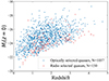 |
Fig. 1. Distribution of the i-band absolute magnitude as a function of redshift. The blue dots and red triangles represent the optically selected and radio selected quasars with the LOFAR detections, respectively. |
3.1. The α − z relationship of quasars
In Figs. 2 and 3 we present the redshift evolution of the spectral index. The number density of our sample peaks between redshift 1 and 2, as illustrated in the top panel of each figure.
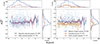 |
Fig. 2. Relationship between the low-frequency spectral index ( |


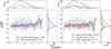 |
Fig. 3. Relationship between the high-frequency spectral index ( |


The spectral index  as a function of redshift is shown in the left panel of Fig. 2. Neither the optical-selected nor radio-selected quasars show a trend with redshift. Additionally, the overall spectral index (
 ) distribution remains constant with redshift, with median values of −0.626 ± 0.004 for optically selected quasars and −0.608 ± 0.011 for radio-selected quasars. These errors were calculated using error propagation (Taylor 1982). The median spectral index appears to increase slightly toward higher redshifts; however, due to the limited sample size around a redshift of 4, a solid conclusion cannot be drawn. In the right panel of Fig. 2, we separate the extended sources from compact sources. Overall, the median spectral index (
 ) of extended sources is steeper than that of compact sources. This difference is not significantly influenced by the potential loss of diffuse emissions, as LOFAR’s extensive short baselines ensure excellent uv coverage, enabling the recovery of such emission (Hoang et al. 2018; Botteon et al. 2020; Shimwell et al. 2022). At low redshifts, the median spectral index of radio compact sources is steeper than that of optical compact sources. Specifically, the median spectral index values for extended, optical compact, and radio compact sources are −0.823 ± 0.012, −0.532 ± 0.011, and −0.567 ± 0.030, respectively.
In Fig. 3, for both samples, the results for the high ν spectral index ( ) are generally consistent with those for the low ν spectral index (
 ). For optical and radio quasars, the median spectral indices are −0.650 ± 0.001 and −0.683 ± 0.002, respectively. The median spectral index of extended sources, with a value of −0.790 ± 0.006, is steeper than that of compact sources: −0.585 ± 0.004 for optical compact sources and −0.655 ± 0.011 for radio compact sources. The median high ν spectral index (
 ) is steeper than the low ν spectral index (
 ) for compact sources. This indicates that the overall radio spectrum of compact sources is flatter at lower frequencies compared to higher frequencies.
3.2. The evolution of MPS sources
In Fig. 4 we present the low ν ( ) and high ν (
 ) spectral index radio color-color diagram. Most sources (around 85.2%) exhibit a negative power-law spectral index in the bottom-left quadrant, consistent with previous work (Callingham et al. 2017). The bottom-right quadrant shows the distribution of MPS sources (around 5.1%). The top-right quadrant shows the GPS and HFP sources (around 2.5%). The top-left quadrant shows the sources with an upturn in their radio spectra (around 4.3%). For the MPS sources, the median
  and
and  are 0.391 ± 0.049 and −0.390 ± 0.013, respectively.
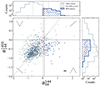 |
Fig. 4. 2D distribution of the spectral index for all quasars in the study. The four quadrants represent different shapes of the radio spectra. The blue stars in the lower-right quadrant are the MPS samples discussed in this paper. Red dots indicate sources that meet |


The fraction of MPS sources (fMPS) as a function of redshift is shown in the left panel of Fig. 5. The main plot shows that for detected sources in the three surveys, their fraction exhibits a peak around redshift 0.5 and 2. This aligns with the peaks around 2 in the distribution of the number of sources as a function of redshift in the subplot. We find that the fraction of MPS sources does not show a clear relationship with redshift, and the same result holds for samples with LoLSS or FIRST flux upper limits in the LoLSS DR1 sky coverage. The high fraction of MPS sources observed at z > 4 is due to the sample number statistics rather than a genuine increase. Additionally, the number of MPS sources drops at z > 3, which is related to the incomplete quasar identification at high redshifts and the limited sky coverage of the survey (Wu & Shen 2022; de Gasperin et al. 2023). In summary, the majority of MPS sources are indeed concentrated between redshift 2 and 3. However, the fraction of MPS sources does not change with redshift.
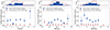 |
Fig. 5. Left to right: Relationships between the fraction of MPS sources and redshift, bolometric luminosity (LBol), and black hole mass (MBH). The blue dots represent sources detected by LoTSS, LoLSS, and FIRST, while the red triangles represent sources detected by LoTSS with LoLSS/FIRST upper limits in the LoLSS DR1 sky coverage. |
In the middle panel of Fig. 5, we show that the fraction of MPS sources (fMPS) does not depend on the bolometric luminosity (LBol), which is derived from the rest-frame optical continuum luminosity (Wu & Shen 2022). Although there is an increase in the last luminosity bin, this is likely due to the limited sample size, as indicated by the large error bars. Therefore, we conclude that the fraction of MPS sources does not significantly change with bolometric luminosity. Since bolometric luminosity (LBol) is related to the properties of SMBHs, such as mass, spin, and accretion rate (Gürkan et al. 2019; Frank et al. 2002), this result suggests that the activities of SMBHs may not strongly influence the formation of MPS sources.
To further investigate the influence of SMBHs, the right panel of Fig. 5 presents the fraction of MPS sources (fMPS) as a function of SMBH mass. These black hole masses, estimated from measurements of the continuum and broad line emissions (Wu & Shen 2022), are concentrated between 108.5 and  . Overall, the fraction of MPS sources remains consistent across different SMBH masses.
4. Discussion
4.1. The constant α − z relationship of quasars
For quasars, we find that both the median  and
and  spectral indices are steeper for extended sources compared to compact sources (Sect. 3.1), which is consistent with previous work. Specifically, for
  , the median value for extended sources is around −0.8 (de Gasperin et al. 2018; Gürkan et al. 2019). For compact sources, studies generally found that the overall spectral index is flatter compared to extended sources. However, the specific results varied across different studies. For instance, in Gürkan et al. (2019), the median values of
  for optical compact and radio compact sources are −0.26 ± 0.02 and −0.36 ± 0.06, respectively. Similarly, in de Gasperin et al. (2018), the spectral index (
 ) for compact sources is −0.5.
The difference in spectral indices between extended and compact sources is believed to be related to the emission originating from different parts of the sources (Urry & Padovani 1995). Flat-spectrum compact sources are likely from core-dominated AGNs, while steep-spectrum extended sources are likely from lobe-dominated regions (Blundell et al. 1999). The radio spectrum of AGN cores is typically flat (around −0.5), whereas the lobes have a steeper spectrum due to synchrotron and inverse Compton aging, also combined with adiabatic expansion (Blundell et al. 1999; de Gasperin et al. 2018).
We also find that the spectral indices ( and
and  ) of quasars do not significantly change with redshift across 0 < z < 5. This result is consistent with the result from Smolčić et al. (2014), who found no clear steepening of
  for AGNs in the VLA-COSMOS field. Similar results were found for star-forming galaxies (
 ; Ivison et al. 2010; Thomson et al. 2014; Magnelli et al. 2015). Ker et al. (2012) also show a weak correlation between these two parameters in complete radio samples with spectral index at different frequencies (e.g.,
  and
and  ).
).
However, previous results found a steepening of spectral indices for radio galaxies at higher redshifts (De Breuck et al. 2000, 2002; Klamer et al. 2006; Singh et al. 2014). This steepening could be attributed to the K-correction of the concave spectrum, increasing environmental density at higher redshifts, or secondary effects of the luminosity-spectral index relationship (Chambers et al. 1990; Athreya et al. 1998; Miley & De Breuck 2008). Since we observed no steepening of the spectral index at lower frequencies for quasars, these mechanisms might not be important for the spectral evolution of quasars. First, the K-correction effect, which causes higher-redshift radio galaxies to appear steeper due to a shift in the observed spectral, may not apply to quasars due to their typically flatter radio spectra (Hutchings 1987; Tadhunter 2016; Gloudemans et al. 2023). Secondly, the environmental density that could cause radio spectral steepening in radio galaxies is likely less impactful for quasars. This is supported by the positive relationship between jet power and radio luminosity (Cavagnolo et al. 2010; Godfrey & Shabala 2016), and the evidence that the quasars studied in this work have a powerful median radio luminosity of log10(L144 MHz) = 26.83 ± 0.86 W/Hz, calculated using data from Hardcastle et al. (2023). Such high radio luminosities indicate that these quasars possess powerful jets. These jets and high-energy emissions make quasars less sensitive to increased environmental density (Lietzen et al. 2009, 2011). Lastly, the luminosity-spectral index relationship may also differ for quasars, which are often dominated by accretion-related emissions rather than lobe-dominated synchrotron emissions, making their spectral evolution less dependent on redshift-related environmental changes (Barthel 1989; Urry & Padovani 1995; Tadhunter 2016). These factors suggest that the steepening mechanisms observed in radio galaxies may not be important for the spectral evolution of quasars.
4.2. The mechanism behind the MPS sources
Two possible absorption scenarios have been proposed to explain the turnover of the radio spectrum. Synchrotron self-absorption occurs when a source is optically thick, in the case of a uniform plasma, leading to a spectral index close to 2.5 at low frequencies (O’Dea & Baum 1997). Free-free absorption is due to photons being absorbed by the ambient dense medium. If the absorption is within the source, the typical spectral index should be 2.1 (Callingham et al. 2015; Keim et al. 2019). The external absorption will make the low-frequency spectral index steeper (Bicknell et al. 1997; Keim et al. 2019).
In this work we identified 61 MPS sources with peaks at the extremely low frequency of 144 MHz. We find that for these sources, the median  is 0.391, which does not allow us to draw definitive conclusions on the general absorption mechanism. The significant discrepancy between the observed spectral index (0.391) and the predicted value (2.1 or 2.5) could be due to our data points being too close to the peak frequency, or possibly because the peak frequency lies within the 54–144 MHz range. Also, the selection effect could impact the detection of MPS sources in this work. As shown in Fig. 6, steep spectral indices (around 2) tend to have higher flux densities at 144 MHz. Thus, identifying the predicted steep spectral indices, such as 2.1 or 2.5, requires that sources are bright in LoTSS. This requirement might contribute to the absence of steep spectral indices observed here. Consequently, the additional data at lower frequencies, such as from the LOFAR Decameter Sky Survey (LoDeSS) with observations between 10 and 30 MHz (Groeneveld et al. 2024) or other data around 100 MHz, would allow us to perform spectral fitting to determine both the peak and the spectral index below the peak more accurately.
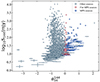 |
Fig. 6. Relationship between the spectral index and flux density at 144 MHz for quasars in this work. The blue stars are the MPS sources discussed in this paper. Red diamonds indicate sources with |


We also find a constant relationship between the fraction of MPS sources and redshift, bolometric luminosity, and SMBH mass. This suggests that the occurrence of MPS sources is relatively independent of cosmic evolution, radiation intensity, and black hole mass, pointing to a distinct physical mechanism that remains stable across different evolutionary stages and environments. This stability aligns with studies indicating that quasar and AGN spectral indices can vary independently of redshift and environmental conditions (Falcke & Biermann 1995; Lietzen et al. 2009, 2011; Tadhunter 2016).
5. Summary
The large quasar sample provided by SDSS and the high-resolution, high-sensitivity, low-frequency radio data from LOFAR and VLA enable us to study the α − z relationship of quasars at frequencies below 100 MHz. We obtained a quasar sample of 1,187 sources with detection in the SDSS, LoLSS, LoTSS, and FIRST surveys. We find constant spectral indices ( and
and  ) as redshift increases (0 < z < 5). Additionally, we confirm that the extended sources in our quasar sample have steeper spectra than compact sources at lower frequencies. This could be explained by the radio emission originating from different regions: the flat spectra would be from the compact core region, and the emission of extended sources are mostly from the lobes.
By employing cuts for spectral indices  and
and  , we identified 61 MPS sources. Our analysis reveals that the fractions of these sources remain constant with redshift, bolometric luminosity, and SMBH mass. These findings suggest that MPS sources are governed by unique physical conditions or formation mechanisms that remain stable across different evolutionary stages and environments. However, it is important to note that the small sample size constrains this analysis. Future work should focus on expanding the sample size and exploring a lower and broader frequency coverage to improve our understanding of the turnover model of MPS sources. Detailed spectral modeling could also help locate the turnover frequency and spectral indices below this frequency. Further analysis of the environment and host galaxy properties may also shed light on the external impact on the formation of MPS sources.
Acknowledgments
We thank the anonymous referee for their valuable comments. SZ thanks Jinyi Liu, Yuming Fu, and Joseph Callingham for their helpful assistance. LOFAR data products were provided by the LOFAR Surveys Key Science project (LSKSP; https://lofar-surveys.org/) and were derived from observations with the International LOFAR Telescope (ILT). LOFAR (van Haarlem et al. 2013) is the Low Frequency Array designed and constructed by ASTRON. It has observing, data processing, and data storage facilities in several countries, which are owned by various parties (each with their own funding sources), and which are collectively operated by the ILT foundation under a joint scientific policy. The efforts of the LSKSP have benefited from funding from the European Research Council, NOVA, NWO, CNRS-INSU, the SURF Co-operative, the UK Science and Technology Funding Council and the Jülich Supercomputing Centre. SZ acknowledges support from the CSC (China Scholarship Council)-Leiden University joint scholarship program. FdG acknowledges the support of the ERC Consolidator Grant ULU 101086378.
References
- An, T., & Baan, W. A. 2012, ApJ, 760, 77 [Google Scholar]
- Athreya, R. M., Kapahi, V. K., McCarthy, P. J., & van Breugel, W. 1998, A&A, 329, 809 [NASA ADS] [Google Scholar]
- Ballieux, F. J., Callingham, J. R., Röttgering, H. J. A., & Slob, M. M. 2024, A&A, 689, A264 [NASA ADS] [CrossRef] [EDP Sciences] [Google Scholar]
- Barthel, P. D. 1989, ApJ, 336, 606 [Google Scholar]
- Becker, R. H., White, R. L., & Helfand, D. J. 1994, in Astronomical Data Analysis Software and Systems III, eds. D. R. Crabtree, R. J. Hanisch, & J. Barnes, ASP Conf. Ser., 61, 165 [NASA ADS] [Google Scholar]
- Becker, R. H., White, R. L., & Helfand, D. J. 1995, ApJ, 450, 559 [Google Scholar]
- Bicknell, G. V., Dopita, M. A., & O’Dea, C. P. O. 1997, ApJ, 485, 112 [NASA ADS] [CrossRef] [Google Scholar]
- Blundell, K. M., Rawlings, S., & Willott, C. J. 1999, AJ, 117, 677 [Google Scholar]
- Botteon, A., Brunetti, G., van Weeren, R. J., et al. 2020, ApJ, 897, 93 [Google Scholar]
- Callingham, J. R., Gaensler, B. M., Ekers, R. D., et al. 2015, ApJ, 809, 168 [Google Scholar]
- Callingham, J. R., Ekers, R. D., Gaensler, B. M., et al. 2017, ApJ, 836, 174 [CrossRef] [Google Scholar]
- Cavagnolo, K. W., McNamara, B. R., Nulsen, P. E. J., et al. 2010, ApJ, 720, 1066 [Google Scholar]
- Chambers, K. C., Miley, G. K., & van Breugel, W. J. M. 1990, ApJ, 363, 21 [NASA ADS] [CrossRef] [Google Scholar]
- Coppejans, R., Cseh, D., Williams, W. L., van Velzen, S., & Falcke, H. 2015, MNRAS, 450, 1477 [Google Scholar]
- Coppejans, R., Cseh, D., van Velzen, S., et al. 2016, MNRAS, 459, 2455 [Google Scholar]
- Dallacasa, D., Stanghellini, C., Centonza, M., & Fanti, R. 2000, A&A, 363, 887 [NASA ADS] [Google Scholar]
- De Breuck, C., van Breugel, W., Röttgering, H. J. A., & Miley, G. 2000, A&AS, 143, 303 [NASA ADS] [CrossRef] [EDP Sciences] [Google Scholar]
- De Breuck, C., van Breugel, W., Stanford, S. A., et al. 2002, AJ, 123, 637 [NASA ADS] [CrossRef] [Google Scholar]
- de Gasperin, F., Intema, H. T., & Frail, D. A. 2018, MNRAS, 474, 5008 [Google Scholar]
- de Gasperin, F., Edler, H. W., Williams, W. L., et al. 2023, A&A, 673, A165 [NASA ADS] [CrossRef] [EDP Sciences] [Google Scholar]
- Falcke, H., & Biermann, P. L. 1995, A&A, 293, 665 [NASA ADS] [Google Scholar]
- Falcke, H., Körding, E., & Nagar, N. M. 2004, New Astron. Rev., 48, 1157 [Google Scholar]
- Fan, X., Carilli, C. L., & Keating, B. 2006, ARA&A, 44, 415 [Google Scholar]
- Fanti, R., Fanti, C., Schilizzi, R. T., et al. 1990, A&A, 231, 333 [NASA ADS] [Google Scholar]
- Frank, J., King, A., & Raine, D. J. 2002, Accretion Power in Astrophysics, Third Edition [Google Scholar]
- Gebhardt, K., Mentuch Cooper, E., Ciardullo, R., et al. 2021, ApJ, 923, 217 [NASA ADS] [CrossRef] [Google Scholar]
- Gloudemans, A. J., Saxena, A., Intema, H., et al. 2023, A&A, 678, A128 [NASA ADS] [CrossRef] [EDP Sciences] [Google Scholar]
- Godfrey, L. E. H., & Shabala, S. S. 2016, MNRAS, 456, 1172 [NASA ADS] [CrossRef] [Google Scholar]
- Groeneveld, C., van Weeren, R. J., Osinga, E., et al. 2024, Nat. Astron., 8, 786 [NASA ADS] [CrossRef] [Google Scholar]
- Gürkan, G., Hardcastle, M. J., Best, P. N., et al. 2019, A&A, 622, A11 [NASA ADS] [CrossRef] [EDP Sciences] [Google Scholar]
- Hardcastle, M. J., Horton, M. A., Williams, W. L., et al. 2023, A&A, 678, A151 [NASA ADS] [CrossRef] [EDP Sciences] [Google Scholar]
- Helfand, D. J., Becker, R. H., White, R. L., et al. 1994, Am. Astron. Soc. Meeting Abstr., 185, 08.03 [NASA ADS] [Google Scholar]
- Helfand, D. J., White, R. L., & Becker, R. H. 2015, ApJ, 801, 26 [NASA ADS] [CrossRef] [Google Scholar]
- Hoang, D. N., Shimwell, T. W., van Weeren, R. J., et al. 2018, MNRAS, 478, 2218 [Google Scholar]
- Hutchings, J. B. 1987, ApJ, 320, 122 [NASA ADS] [CrossRef] [Google Scholar]
- Ivison, R. J., Alexander, D. M., Biggs, A. D., et al. 2010, MNRAS, 402, 245 [Google Scholar]
- Keim, M. A., Callingham, J. R., & Röttgering, H. J. A. 2019, A&A, 628, A56 [NASA ADS] [CrossRef] [EDP Sciences] [Google Scholar]
- Ker, L. M., Best, P. N., Rigby, E. E., Röttgering, H. J. A., & Gendre, M. A. 2012, MNRAS, 420, 2644 [NASA ADS] [CrossRef] [Google Scholar]
- Klamer, I. J., Ekers, R. D., Bryant, J. J., et al. 2006, MNRAS, 371, 852 [Google Scholar]
- Knuth, K. H. 2006, ArXiv e-prints [arXiv:physics/0605197] [Google Scholar]
- Kormendy, J., & Richstone, D. 1995, ARA&A, 33, 581 [Google Scholar]
- Kunert-Bajraszewska, M., Gawroński, M. P., Labiano, A., & Siemiginowska, A. 2010, MNRAS, 408, 2261 [NASA ADS] [CrossRef] [Google Scholar]
- Lietzen, H., Heinämäki, P., Nurmi, P., et al. 2009, A&A, 501, 145 [NASA ADS] [CrossRef] [EDP Sciences] [Google Scholar]
- Lietzen, H., Heinämäki, P., Nurmi, P., et al. 2011, A&A, 535, A21 [NASA ADS] [CrossRef] [EDP Sciences] [Google Scholar]
- Lyke, B. W., Higley, A. N., McLane, J. N., et al. 2020, ApJS, 250, 8 [NASA ADS] [CrossRef] [Google Scholar]
- Magnelli, B., Ivison, R. J., Lutz, D., et al. 2015, A&A, 573, A45 [NASA ADS] [CrossRef] [EDP Sciences] [Google Scholar]
- Marr, J. M., Perry, T. M., Read, J., Taylor, G. B., & Morris, A. O. 2014, ApJ, 780, 178 [Google Scholar]
- Miley, G., & De Breuck, C. 2008, A&ARv, 15, 67 [Google Scholar]
- Mohan, N., & Rafferty, D. 2015, Astrophysics Source Code Library [record ascl:1502.007] [Google Scholar]
- Murgia, M., Fanti, C., Fanti, R., et al. 2002, New Astron. Rev., 46, 307 [CrossRef] [Google Scholar]
- Myers, A. D., Palanque-Delabrouille, N., Prakash, A., et al. 2015, ApJS, 221, 27 [NASA ADS] [CrossRef] [Google Scholar]
- O’Dea, C. P. 1998, PASP, 110, 493 [Google Scholar]
- O’Dea, C. P., & Baum, S. A. 1997, AJ, 113, 148 [CrossRef] [Google Scholar]
- O’Dea, C. P., Baum, S. A., & Stanghellini, C. 1991, ApJ, 380, 66 [CrossRef] [Google Scholar]
- Owen, F. N., Morrison, G. E., Klimek, M. D., & Greisen, E. W. 2009, AJ, 137, 4846 [Google Scholar]
- Planck Collaboration XIII. 2016, A&A, 594, A13 [NASA ADS] [CrossRef] [EDP Sciences] [Google Scholar]
- Rees, M. J. 1984, ARA&A, 22, 471 [Google Scholar]
- Richards, G. T., Strauss, M. A., Fan, X., et al. 2006, AJ, 131, 2766 [Google Scholar]
- Schmidt, M. 1963, Nature, 197, 1040 [Google Scholar]
- Shields, G. A. 1999, PASP, 111, 661 [NASA ADS] [CrossRef] [Google Scholar]
- Shimwell, T. W., Tasse, C., Hardcastle, M. J., et al. 2019, A&A, 622, A1 [NASA ADS] [CrossRef] [EDP Sciences] [Google Scholar]
- Shimwell, T. W., Hardcastle, M. J., Tasse, C., et al. 2022, A&A, 659, A1 [NASA ADS] [CrossRef] [EDP Sciences] [Google Scholar]
- Singh, V., Beelen, A., Wadadekar, Y., et al. 2014, A&A, 569, A52 [NASA ADS] [CrossRef] [EDP Sciences] [Google Scholar]
- Slob, M. M., Callingham, J. R., Röttgering, H. J. A., et al. 2022, A&A, 668, A186 [NASA ADS] [CrossRef] [EDP Sciences] [Google Scholar]
- Smolčić, V., Ciliegi, P., Jelić, V., et al. 2014, MNRAS, 443, 2590 [CrossRef] [Google Scholar]
- Snellen, I. A. G., Schilizzi, R. T., Miley, G. K., et al. 2000, MNRAS, 319, 445 [NASA ADS] [CrossRef] [Google Scholar]
- Tadhunter, C. 2016, A&ARv, 24, 10 [Google Scholar]
- Taylor, J. R. 1982, An Introduction to Error Analysis: The Study of Uncertainties in Physical Measurements (University Science Books) [Google Scholar]
- Thomson, A. P., Ivison, R. J., Simpson, J. M., et al. 2014, MNRAS, 442, 577 [NASA ADS] [CrossRef] [Google Scholar]
- Urry, C. M., & Padovani, P. 1995, PASP, 107, 803 [NASA ADS] [CrossRef] [Google Scholar]
- van Breugel, W., Miley, G., & Heckman, T. 1984, AJ, 89, 5 [Google Scholar]
- van Haarlem, M. P., Wise, M. W., Gunst, A. W., et al. 2013, A&A, 556, A2 [NASA ADS] [CrossRef] [EDP Sciences] [Google Scholar]
- Wang, F., Yang, J., Fan, X., et al. 2021, ApJ, 907, L1 [Google Scholar]
- Wu, Q., & Shen, Y. 2022, ApJS, 263, 42 [NASA ADS] [CrossRef] [Google Scholar]
- Yang, J., Wang, F., Fan, X., et al. 2020, ApJ, 897, L14 [Google Scholar]
All Tables
All Figures
|
Fig. 1. Distribution of the i-band absolute magnitude as a function of redshift. The blue dots and red triangles represent the optically selected and radio selected quasars with the LOFAR detections, respectively. |
| In the text | |
|
Fig. 2. Relationship between the low-frequency spectral index ( |
| In the text | |
|
Fig. 3. Relationship between the high-frequency spectral index ( |
| In the text | |
|
Fig. 4. 2D distribution of the spectral index for all quasars in the study. The four quadrants represent different shapes of the radio spectra. The blue stars in the lower-right quadrant are the MPS samples discussed in this paper. Red dots indicate sources that meet |
| In the text | |
|
Fig. 5. Left to right: Relationships between the fraction of MPS sources and redshift, bolometric luminosity (LBol), and black hole mass (MBH). The blue dots represent sources detected by LoTSS, LoLSS, and FIRST, while the red triangles represent sources detected by LoTSS with LoLSS/FIRST upper limits in the LoLSS DR1 sky coverage. |
| In the text | |
|
Fig. 6. Relationship between the spectral index and flux density at 144 MHz for quasars in this work. The blue stars are the MPS sources discussed in this paper. Red diamonds indicate sources with |
| In the text | |
Current usage metrics show cumulative count of Article Views (full-text article views including HTML views, PDF and ePub downloads, according to the available data) and Abstracts Views on Vision4Press platform.
Data correspond to usage on the plateform after 2015. The current usage metrics is available 48-96 hours after online publication and is updated daily on week days.
Initial download of the metrics may take a while.