| Issue |
A&A
Volume 695, March 2025
|
|
|---|---|---|
| Article Number | L6 | |
| Number of page(s) | 8 | |
| Section | Letters to the Editor | |
| DOI | https://doi.org/10.1051/0004-6361/202452851 | |
| Published online | 28 February 2025 | |
Letter to the Editor
14N/15N abundance ratio toward massive star-forming regions with different Galactic distances
1
Guangxi Key Laboratory for Relativistic Astrophysics, School of Physical Science and Technology, Guangxi University, Nanning 530004, China
2
Shanghai Astronomical Observatory, Chinese Academy of Sciences, 80 Nandan Road, Shanghai 200030, China
3
Key Laboratory of Radio Astronomy, Chinese Academy of Sciences, Nanjing 210033, China
⋆ Corresponding authors; junzhiwang@gxu.edu.cn; changruan@st.gxu.edu.cn
Received:
2
November
2024
Accepted:
3
February
2025
Context. The abundance ratio of 14N/15N is, in principle, a powerful tool for tracing stellar nucleosynthesis.
Aims. This work aims to measure and analyze (14N/15N) × (13C/12C) and 14N/15N abundance ratios in massive star-forming regions across a range of galactocentric distances to provide constraints on galactic chemical evolution (GCE) models.
Methods. We present H13CN and HC15N J = 2–1 results toward 51massive star-forming regions obtained with the Institut de Radioastronomie Millimétrique (IRAM) 30 meter telescope. We used these results to derive (14N/15N) × (13C/12C) abundance ratios as well as 14N/15N ratios using the double isotope method.
Results. We find an overall decreasing trend in the (14N/15N) × (13C/12C) abundance ratio and an increasing trend in the 14N/15N ratio with increasing galactocentric distance (DGC), which provides a good constraint for the GCE model based on high signal to noise ratio measurements. While the predicted (14N/15N) × (13C/12C) ratios between 6 and 12 kpc determined using current GCE models are consistent with our observational results, the ratios from models for DGC less than 6 kpc are significantly higher than the observational results, which indicates GCE models for 14N/15N and/or 13C/12C ratios need to be updated for at least this range.
Key words: stars: evolution / ISM: abundances / Galaxy: abundances / Galaxy: evolution
© The Authors 2025
 Open Access article, published by EDP Sciences, under the terms of the Creative Commons Attribution License (https://creativecommons.org/licenses/by/4.0), which permits unrestricted use, distribution, and reproduction in any medium, provided the original work is properly cited.
This article is published in open access under the Subscribe to Open model. Subscribe to A&A to support open access publication.
1. Introduction
Galactic chemical evolution (GCE) models, which track the distribution of chemical elements of the interstellar medium in galaxies and their formation in stars (Matteucci 2021), help us understand the evolution of stars and galaxies (Tinsley 1980; Matteucci 2021). Carbon, nitrogen, and oxygen in the interstellar medium originate from the evolution of stars via nucleosynthesis processes (Burbidge et al. 1957; Wallerstein et al. 1997). The triple-α capture process leads to the formation of 12C (Salpeter 1952),
while isotopes 13C, 15N, and 17O are produced in hydrogen-burning zones through either the cold or hot CNO cycles (Wiescher et al. 2010; Romano 2022 provides a comprehensive review of CNO nucleosynthesis in stars). Throughout their evolutionary phases, stars release these nucleosynthetic products into the surrounding medium, notably during the asymptotic giant branch and supernova phases (see, e.g., Nomoto et al. 2013; Di Criscienzo et al. 2016; Woosley 2019).
The isotopic abundance ratios of carbon, nitrogen, and oxygen depend heavily on the growth history of the Galactic disk and thus exhibit strong evolutionary features (e.g., Romano & Matteucci 2003; Romano et al. 2017). On various timescales, stars with variable initial masses and chemical compositions create isotopes of different species in varying amounts (Tinsley 1979; Wannier 1980). Hence, measuring the isotopic abundance ratio is an efficient method for tracing the chemical history and constraining GCE models (Wilson & Rood 1994; Romano 2022). For example, the 12C/13C ratio is the consequence of contributions from stars of varying masses, which collectively contribute to the current radial gradient in the Milky Way over different timescales (Milam et al. 2005; Yan et al. 2019). The 18O/17O ratio can be used to trace stellar nucleosynthesis and metal enrichment processes (Henkel et al. 1994; Wilson & Rood 1994; Jiménez-Donaire et al. 2017; Ou et al. 2023). The 14N/15N ratio can also be used to study stellar nucleosynthesis and constrain the latest GCE models (Ritchey et al. 2015; Colzi et al. 2022). 14N is produced through processes like hot bottom burning in asymptotic giant branch stars (Renzini & Voli 1981; Romano 2022) and the cold CNO cycle during hydrogen-burning stages (Colzi et al. 2018b), while 15N is mainly formed in nova outbursts via the hot CNO cycle (Clayton 2003; Colzi et al. 2018b).
The abundance ratio of isotopes can be obtained using three alternative approaches: the singly substituted molecules, doubly substituted molecules, and double isotope methods (Wampfler et al. 2014). For the singly substituted molecules method, which involves molecules such as CN/C15N (see, e.g., Adande & Ziurys 2012; Ritchey et al. 2015; Sun et al. 2024), the main isotopologs are usually abundant, resulting in strong lines. However, a high abundance frequently means a high optical depth, which must be corrected via radiative transfer modeling or the intensity ratios of the hyperfine transitions (Wampfler et al. 2014). The lines of doubly substituted molecules such as C18O/13C18O (see, e.g., Paron et al. 2018; Jiménez-Donaire et al. 2017) are usually very weak as a result of their low abundances. The double isotope method, which involves, for example, HN13C/H15NC or H13CN/HC15N (see, e.g., Adande & Ziurys 2012; Wampfler et al. 2014; Colzi et al. 2018a,b, 2022), avoids the high opacities of the main isotopolog and the weak lines of doubly substituted molecules. However, the abundance ratio of 12C/13C must be known to derive the 14N/15N ratio.
We used the double isotope method to derive 14N/15N ratios from the intensity ratio of H13CN/HC15N J = 2–1 lines. Assuming H13CN and HC15N 2–1 to be optically thin with similar excitation properties, the abundance ratios of 14N/15N can be derived from velocity-integrated intensities of H13CN/HC15N 2–1 by multiplying by 12C/13C (see, e.g., Goldsmith et al. 1981; Wampfler et al. 2014) as a function of DGC,
The 12C/13C value in each source was obtained from Sun et al. (2024) as

We report the abundance ratios of 14N/15N derived using the double isotope method from data obtained with the Institut de Radioastronomie Millimétrique (IRAM) 30 m telescope toward 51 massive star-forming regions. The IRAM 30 m observations are described in Sect. 2. Section 3 provides a description of the main results. A discussion and our conclusions are presented in Sects. 4 and 5.
2. Observation
2.1. IRAM 30 m observations
The sample of 51 late-stage massive star-forming regions with parallactic distances from Reid et al. (2014, 2019) was selected to observe the spectral lines of H13CN J = 2–1 at 172.6778512 GHz and HC15N J = 2–1 at 172.1079571 GHz using the IRAM 30 meter telescope on Pico Veleta, Spain. The observations were carried out in June 2016, October 2016, and August 2017, except for G211.59+01.05, which was observed in August 2020. These sources, except for G211.59+01.05, are the same as those presented in Li et al. (2022) for NH2D molecules. The 2 mm (E1) band of the Eight Mixer Receiver (EMIR) and the Fourier Transform Spectrometers (FTS) backend were used to cover from about 166.0 GHz–173.8 GHz with 195 kHz channel spacing and dual polarization. The standard position-switching mode with an azimuth OFF of −600 arcsec was used.
The IRAM 30 m telescope, with a beam size of ∼14.3 arcsec at 172 GHz and a typical system temperature of 400 K in the 2 mm band, utilizes nearby quasi-stellar objects for pointing correction every two hours. Focus was checked and corrected at the start of each run, as well as during sunsets and sunrises. The main beam brightness temperature (Tmb) was calculated using  , where
  is the antenna temperature, the forward efficiency (Feff) is 0.93, and the beam efficiency (Beff) is 0.73 for the 2 mm band. Each scan lasted 2 minutes, and the total on-source time ranged from 12 to 234 minutes per source.
2.2. Data reduction
Data reduction was based on the CLASS package in the GILDAS1 software, a comprehensive tool designed for (sub)millimeter radio-astronomical applications, which facilitates the efficient manipulation and visualization of spectra. GILDAS is widely used to process data from the IRAM 30 m telescope and the NOrthern Extended Millimeter Array (NOEMA), excluding very long-baseline interferometry observations. The spectra from each source were averaged into one spectrum using the CLASS package and subtracted from a first-order baseline. The spectra in each source were plotted on the same velocity scale to facilitate comparisons between H13CN and HC15N J = 2–1. The line fluxes were determined through a direct integration of the emission lines, with errors calculated using the equation  , where δv represents the channel separation in velocity, Δv the velocity range for integration, and rms the root mean square noise obtained with baseline fitting for each spectrum with δv channel spacing.
3. Results
The spectra with Tpeak > 3σ at 195 kHz channel spacing, which corresponds to 0.34 km s−1 at 172 GHz, were considered detections, where Tpeak is peak Tmb and σ is the rms noise. Neither H13CN J = 2–1 nor HC15N J = 2–1 were detected in IRAS 05137+3919 or G012.90-00.24. HC15N J = 2–1 was not detected, while a clear double-peak structure of H13CN J = 2–1 was found in Sgr B2, which was likely due to the self-absorption of hot core regions (see, e.g., Adande & Ziurys 2012). Both H13CN J = 2–1 and HC15N J = 2–1 lines were contaminated by nearby lines in G010.47+00.02, which hindered the use of these two lines for scientific analysis. H13CN J = 2–1 and HC15N J = 2–1 were detected and included in the ratio calculations for the remaining 47 sources.
The velocity-integrated intensities of H13CN J = 2–1 range from 1.6 ± 0.03 K km s−1 in G211.59+01.05 to 115.7 ± 0.7 K km s−1 in G005.88−00.39, with a mid-value of 10.9 ± 0.1 K km s−1, as shown in Table A.1. The velocity-integrated intensities of HC15N J = 2–1 range from 0.3 ± 0.03 K km s−1 in G211.59+01.05 to 38.2 ± 0.2 K km s−1 in W51M, with a mid-value of 2.4 ± 0.1 K km s−1.
The hyperfine structure (hfs) of H13CN 2–1 (Fuchs et al. 2004; Cazzoli & Puzzarini 2005) can cause an overestimation of line widths if single-component Gaussians are used. Thus, only full widths at half maximum (FWHMs) of HC15N J = 2–1 in each source were derived through single-component Gaussian fitting using the CLASS package. The derived FWHMs of HC15N J = 2–1 range from 2.0 ± 0.2 km s−1 in G183.72−03.66 to 15.8 ± 0.2 km s−1 in W49N, with a mid-value of 4.6 ± 0.5 km s−1. Obvious hfs features of H13CN J = 2–1 were found in 16 sources with HC15N J = 2–1 FWHMs less than 5.3 km s−1, but they were blurred into component due to line broadening. Figure 1a shows an example of this, with the H13CN J = 2–1 spectrum in G081.87+00.78. Another example (G081.75+00.59), in which the hfs feature of H13CN J = 2–1 can be distinguished, is shown in Fig. 1b.
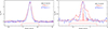 |
Fig. 1. Spectra of H13CN J = 2–1 and HC15N J = 2–1 for two sources as examples. Left: H13CN J = 2–1 hfs in G081.87+00.78 cannot be resolved due to line broadening. Right: H13CN J = 2–1 hfs in G081.75+00.59 can be resolved with a narrow line width. The vertical bold red lines indicate the hyperfine transitions for H13CN J = 2–1: F = 1–1, 1–2, 3–2, 2–1, 1–0, and 2–2 (from left to right). |
The line ratio of H13CN/HC15N 2–1 can be used as the abundance ratio of (14N/15N) × (13C/12C) (Goldsmith et al. 1981), assuming the molecular isotopic abundances ratio represents the isotopic ratio of elements, the same excitation condition as H13CN and HC15N molecules, and both lines are optically thin. The relationship between the (14N/15N) × (13C/12C) abundance ratio derived from the H13CN/HC15N 2–1 line ratio and DGC, as well as the 14N/15N ratios and DGC, is presented in Fig. 2. The DGC values range from 3.3 kpc in G009.62+00.19 to 11.9 kpc in G211.59+01.05 (Reid et al. 2014, 2019). The (14N/15N) × (13C/12C) ratio varies from 2.5 ± 0.02 in W51M to 9.2 ± 0.8 in G023.44−00.18. The unweighted linear regression fits to these data were obtained as follows:
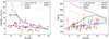 |
Fig. 2. Abundance ratios of (14N/15N) × (13C/12C) (left) and 14N/15N with DGC (right). The filled black circles are sources with peak Tmb of H13CN 2–1 lower than 4 K, and the orange stars sources with peak Tmb higher than 4 K. The blue lines are linear fitting results. The cyan parabola was obtained by multiplying the linear regression fit of (14N/15N) × (13C/12C) given in Eq. (3) by the 12C/13C ratio (Eq. (2)). The green, dark green, pink, and magenta lines are the models from Colzi et al. (2022). |

with a correlation coefficient of −0.34.
The relation between DGC and the 14N/15N ratio, derived from the (14N/15N)×(13C/12C) ratio by multiplying by Eq. (2), spans from 109.6 in W51M to 344.6
 in G034.39+00.22. It is presented in Fig. 2b. The unweighted linear regression fits for these data are

As shown in Figs. 2a and 2b, there is a significant decreasing trend in (14N/15N) × (13C/12C) and an increasing trend in 14N/15N ratios with increasing DGC. The (14N/15N) × (13C/12C) ratio versus the heliocentric distance instead of DGC is presented in Fig. 3, which does not show any significant trend.
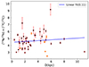 |
Fig. 3. Abundance ratio of (14N/15N) × (13C/12C) versus heliocentric distance. The symbols are the same as in Fig. 2, and the blue line is the linear fitting result. |
4. Discussion
The (14N/15N) × (13C/12C) ratios derived from the observed H13CN/HC15N 2–1 line ratio versus DGC in these 47 sources are compared with four GCE models, shown in Fig. 2, with DGC ranging from 4 to 12 kpc with data points for each 2 kpc (Colzi et al. 2022), in which different initial mass ranges for nova system white dwarf progenitors and various masses ejected in the form of 13C and 15N in each outburst were considered. The decreasing trend in the (14N/15N) × (13C/12C) ratio with increments of DGC in the four models is consistent with our observational results (see Fig. 2a). On the other hand, the poor correlation coefficient between the (14N/15N) × (13C/12C) ratio and the source distance (see Fig. 3) indicates that the decreasing trend in the (14N/15N) × (13C/12C) ratio with increments of DGC is not caused by observational effects of difference source distances to the Sun.
The overall model values of the (14N/15N) × (13C/12C) ratio are higher than the measured ones (see Fig. 2a), which may be caused by the underestimation of the H13CN/HC15N ratio since H13CN J = 2–1 lines are not really optically thin in many sources, especially for sources with strong H13CN 2–1 emission. There are six sources with peak H13CN 2–1 Tmb values higher than 4 K. Because of the possible underestimation of the H13CN/HC15N ratio caused by the moderate opacity of H13CN J = 2–1, our observational results in the range 6–12 kpc should be considered to be generally consistent with the models since they follow a similar trend. However, the (14N/15N) × (13C/12C) ratios predicted by all four models are significantly higher than the observational results, except for that in G023.44–00.18, which has a large error bar. We suggest that the model results of the 14N/15N and/or 13C/12C ratios at 4 kpc need to be updated. Similar results of low (14N/15N) × (13C/12C) ratios in three sources (IRAS 15567−5236, IRAS 17160−3707, and IRAS 17220−3609) with small DGC had been reported, with H13CN and HC15N 1–0 observations (Dahmen et al. 1995). However, no scientific comparisons of observational and model results are available for these sources (Dahmen et al. 1995), mainly because the models had not been developed by that time.
The 14N/15N ratio in each source can be derived using the already obtained (14N/15N) × (13C/12C) ratios and the 13C/12C ratio, which is unknown. We obtained the 14N/15N ratio of each source by assuming the 13C/12C ratio is related to DGC and using the fitting result from Sun et al. (2024), we which plot in Fig. 2b. The slightly tighter correlation between the 14N/15N and the DGC, with a correlation coefficient of 0.42, than that of (14N/15N) × (13C/12C) and DGC, with a correlation coefficient of −0.34, is due to the use of the 13C/12C ratio from the fitting result in Sun et al. (2024). An accurate 14N/15N ratio for each source should be obtained with the measured 13C/12C value in individual sources. Even though the comparison between measured and model ratios of (14N/15N) × (13C/12C) versus DGC should be more accurate than that of the 14N/15N ratio versus DGC, due to the uncertainties of the assumed 13C/12C ratio, the relation between 14N/15N and DGC (see Fig. 2b) can help us find the differences between the four models. When the assumed 13C/12C ratio from Sun et al. (2024) is similar to that of the real value in each source, the 14N/15N ratios from observational results are generally consistent with models 1 and 2. However, they are significantly different to that at 4 and 6 kpc with models 3 and 4, which should therefore be updated.
The range in DGC in our sample is similar to that in Colzi et al. (2018b), while sources with DGC from 12 kpc to 19 kpc were included in Colzi et al. (2022). However, the (14N/15N) × (13C/12C) ratio has much lower uncertainties thanks to the longer typical observing time on each source than that in Colzi et al. (2018b), and as such our results can better constrain predicted (14N/15N) × (13C/12C) and 14N/15N ratios from GCE models, especially when DGC is less than 6 kpc, using the values measured in each source. Future observations with other tracers, which can avoid optically thick effects, will be useful for deriving more accurate 14N/15N ratios than observations with H13CN lines. GCE models of the relation between chemical abundances and DGC were also tested with various tracers in ionized gas, such as radio recombination lines (RRLs; Balser et al. 2011), RRLs and optical lines (Méndez-Delgado et al. 2022), and RRLs and infrared hfs lines (Pineda et al. 2024). The relationship between N/H and DGC shows a clear gradient in regions of DGC greater than 6 kpc, consistent with GCE models, while large scatter is found for DGC less than ∼6 kpc (Pineda et al. 2024). The He, C, N, O, Ne, S, Cl, and Ar abundances varying with DGC (Méndez-Delgado et al. 2022) agrees well with GCE models for DGC greater than 6 kpc; however, they lack data points with DGC less than 6 kpc, mainly because of dust obscuration in the Galactic plane. Thus, isotopic ratios in the regions with DGC less than 6 kpc in molecular gas derived with millimeter wavelengths are ideal for constraining GCE models.
5. Summary and conclusion
H13CN 2–1 and HC15N 2–1 lines are detected in 47 of the 51 massive star-forming regions observed with the IRAM 30 m telescope, and they were used to derive the abundance ratios of (14N/15N) × (13C/12C) as well as 14N/15N via the double isotope method and assumed 13C/12C ratio. The (14N/15N) × (13C/12C) ratio shows a decreasing trend with increasing DGC, while no trend is found for this ratio and distance from the Sun. The 14N/15N ratio shows an increasing trend with increasing DGC. With a small error bar for the measured (14N/15N) × (13C/12C) ratio, our results can constrain the GCE model of (14N/15N) × (13C/12C) well, especially for DGC less than 6 kpc; for that range, updated GCE models are needed.
Acknowledgments
We thank Dr. Donatella Romano for helpful discussion and provide the data GCE model. This work is supported by National Key R & D Program of China under grant 2023YFA1608204 and the National Natural Science Foundation of China grant 12173067. This work is based on observations carried out under project numbers 012-16, 023-17, and 005-20, with the IRAM 30m telescope. IRAM is supported by INSU/CNRS (France), MPG (Germany) and IGN (Spain).
References
- Adande, G. R., & Ziurys, L. M. 2012, ApJ, 744, 194 [NASA ADS] [CrossRef] [Google Scholar]
- Balser, D. S., Rood, R. T., Bania, T. M., & Anderson, L. D. 2011, ApJ, 738, 27 [NASA ADS] [CrossRef] [Google Scholar]
- Burbidge, E. M., Burbidge, G. R., Fowler, W. A., & Hoyle, F. 1957, Reviews of Modern Physics, 29, 547 [CrossRef] [Google Scholar]
- Cazzoli, G., & Puzzarini, C. 2005, Journal of Molecular Spectroscopy, 233, 280 [NASA ADS] [CrossRef] [Google Scholar]
- Clayton, D. 2003, Handbook of Isotopes in the Cosmos (Cambridge: Cambridge University Press) [Google Scholar]
- Colzi, L., Fontani, F., Caselli, P., et al. 2018a, A&A, 609, A129 [NASA ADS] [CrossRef] [EDP Sciences] [Google Scholar]
- Colzi, L., Fontani, F., Rivilla, V. M., et al. 2018b, MNRAS, 478, 3693 [Google Scholar]
- Colzi, L., Romano, D., Fontani, F., et al. 2022, A&A, 667, A151 [NASA ADS] [CrossRef] [EDP Sciences] [Google Scholar]
- Dahmen, G., Wilson, T. L., & Matteucci, F. 1995, A&A, 295, 194 [NASA ADS] [Google Scholar]
- Di Criscienzo, M., Ventura, P., García-Hernández, D. A., et al. 2016, MNRAS, 462, 395 [NASA ADS] [CrossRef] [Google Scholar]
- Fuchs, U., Brünken, S., Fuchs, G., et al. 2004, Zeitschrift für Naturforschung A, 59, 861 [CrossRef] [Google Scholar]
- Goldsmith, P. F., Langer, W. D., Ellder, J., Kollberg, E., & Irvine, W. 1981, ApJ, 249, 524 [Google Scholar]
- Henkel, C., Wilson, T. L., Langer, N., Chin, Y. N., & Mauersberger, R. 1994, in The Structure and Content of Molecular Clouds, eds. T. L. Wilson, & K. J. Johnston, 439, 72 [Google Scholar]
- Jiménez-Donaire, M. J., Cormier, D., Bigiel, F., et al. 2017, ApJ, 836, L29 [Google Scholar]
- Li, Y., Wang, J., Li, J., Liu, S., & Luo, Q. 2022, MNRAS, 512, 4934 [NASA ADS] [CrossRef] [Google Scholar]
- Matteucci, F. 2021, A&ARv, 29, 5 [NASA ADS] [CrossRef] [Google Scholar]
- Méndez-Delgado, J. E., Amayo, A., Arellano-Córdova, K. Z., et al. 2022, MNRAS, 510, 4436 [CrossRef] [Google Scholar]
- Milam, S. N., Savage, C., Brewster, M. A., Ziurys, L. M., & Wyckoff, S. 2005, ApJ, 634, 1126 [Google Scholar]
- Nomoto, K., Kobayashi, C., & Tominaga, N. 2013, ARA&A, 51, 457 [CrossRef] [Google Scholar]
- Ou, C., Wang, J., Zheng, S., et al. 2023, MNRAS, 522, 559 [NASA ADS] [CrossRef] [Google Scholar]
- Paron, S., Areal, M. B., & Ortega, M. E. 2018, A&A, 617, A14 [NASA ADS] [CrossRef] [EDP Sciences] [Google Scholar]
- Pineda, J. L., Horiuchi, S., Anderson, L. D., et al. 2024, ApJ, 973, 89 [NASA ADS] [CrossRef] [Google Scholar]
- Reid, M. J., Menten, K. M., Brunthaler, A., et al. 2014, ApJ, 783, 130 [Google Scholar]
- Reid, M. J., Menten, K. M., Brunthaler, A., et al. 2019, ApJ, 885, 131 [Google Scholar]
- Renzini, A., & Voli, M. 1981, A&A, 94, 175 [NASA ADS] [Google Scholar]
- Ritchey, A. M., Federman, S. R., & Lambert, D. L. 2015, ApJ, 804, L3 [NASA ADS] [CrossRef] [Google Scholar]
- Romano, D. 2022, A&ARv, 30, 7 [NASA ADS] [CrossRef] [Google Scholar]
- Romano, D., & Matteucci, F. 2003, MNRAS, 342, 185 [Google Scholar]
- Romano, D., Matteucci, F., Zhang, Z.-Y., Papadopoulos, P. P., & Ivison, R. J. 2017, MNRAS, 470, 401 [NASA ADS] [CrossRef] [Google Scholar]
- Salpeter, E. E. 1952, ApJ, 115, 326 [NASA ADS] [CrossRef] [Google Scholar]
- Sun, Y., Zhang, Z.-Y., Wang, J., et al. 2024, MNRAS [Google Scholar]
- Tinsley, B. M. 1979, ApJ, 229, 1046 [Google Scholar]
- Tinsley, B. M. 1980, Fund. Cosmic Phys., 5, 287 [Google Scholar]
- Wallerstein, G., Iben, I., Parker, P., et al. 1997, Reviews of Modern Physics, 69, 995 [NASA ADS] [CrossRef] [Google Scholar]
- Wampfler, S. F., Jørgensen, J. K., Bizzarro, M., & Bisschop, S. E. 2014, A&A, 572, A24 [NASA ADS] [CrossRef] [EDP Sciences] [Google Scholar]
- Wannier, P. G. 1980, ARA&A, 18, 399 [NASA ADS] [CrossRef] [Google Scholar]
- Wiescher, M., Görres, J., Uberseder, E., Imbriani, G., & Pignatari, M. 2010, Annual Review of Nuclear and Particle Science, 60, 381 [NASA ADS] [CrossRef] [Google Scholar]
- Wilson, T. L., & Rood, R. 1994, ARA&A, 32, 191 [Google Scholar]
- Woosley, S. E. 2019, ApJ, 878, 49 [Google Scholar]
- Yan, Y. T., Zhang, J. S., Henkel, C., et al. 2019, ApJ, 877, 154 [Google Scholar]
Appendix A: Data parameters
Source names, equatorial coordinates, distances, molecular species, and ratio data.
Same as Table A.1 but for the four sources excluded from the ratio calculations.
Appendix B: Spectral lines
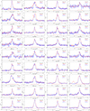 |
Fig. B.1. Observational results of spectra for H13CN 2-1 and HC15N 2-1. They are plotted on the same velocity scale for each spectrum, with the red boxes below each spectrum indicating the velocity integration range for H13CN J = 2–1. |
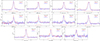 |
Fig. B.1. continued. |
 |
Fig. B.2. Four sources (IRAS 05137+3919, G012.90-00.24, Sgr B2, and G010.47+00.02) excluded from the ratio calculations due to non-detections or contamination in the H13CN J = 2-1 and/or HC15N J = 2-1 lines. |
All Tables
Source names, equatorial coordinates, distances, molecular species, and ratio data.
Same as Table A.1 but for the four sources excluded from the ratio calculations.
All Figures
|
Fig. 1. Spectra of H13CN J = 2–1 and HC15N J = 2–1 for two sources as examples. Left: H13CN J = 2–1 hfs in G081.87+00.78 cannot be resolved due to line broadening. Right: H13CN J = 2–1 hfs in G081.75+00.59 can be resolved with a narrow line width. The vertical bold red lines indicate the hyperfine transitions for H13CN J = 2–1: F = 1–1, 1–2, 3–2, 2–1, 1–0, and 2–2 (from left to right). |
| In the text | |
|
Fig. 2. Abundance ratios of (14N/15N) × (13C/12C) (left) and 14N/15N with DGC (right). The filled black circles are sources with peak Tmb of H13CN 2–1 lower than 4 K, and the orange stars sources with peak Tmb higher than 4 K. The blue lines are linear fitting results. The cyan parabola was obtained by multiplying the linear regression fit of (14N/15N) × (13C/12C) given in Eq. (3) by the 12C/13C ratio (Eq. (2)). The green, dark green, pink, and magenta lines are the models from Colzi et al. (2022). |
| In the text | |
|
Fig. 3. Abundance ratio of (14N/15N) × (13C/12C) versus heliocentric distance. The symbols are the same as in Fig. 2, and the blue line is the linear fitting result. |
| In the text | |
|
Fig. B.1. Observational results of spectra for H13CN 2-1 and HC15N 2-1. They are plotted on the same velocity scale for each spectrum, with the red boxes below each spectrum indicating the velocity integration range for H13CN J = 2–1. |
| In the text | |
|
Fig. B.1. continued. |
| In the text | |
|
Fig. B.2. Four sources (IRAS 05137+3919, G012.90-00.24, Sgr B2, and G010.47+00.02) excluded from the ratio calculations due to non-detections or contamination in the H13CN J = 2-1 and/or HC15N J = 2-1 lines. |
| In the text | |
Current usage metrics show cumulative count of Article Views (full-text article views including HTML views, PDF and ePub downloads, according to the available data) and Abstracts Views on Vision4Press platform.
Data correspond to usage on the plateform after 2015. The current usage metrics is available 48-96 hours after online publication and is updated daily on week days.
Initial download of the metrics may take a while.