| Issue |
A&A
Volume 695, March 2025
|
|
|---|---|---|
| Article Number | A274 | |
| Number of page(s) | 13 | |
| Section | Stellar structure and evolution | |
| DOI | https://doi.org/10.1051/0004-6361/202452660 | |
| Published online | 26 March 2025 | |
Mass loss along the red giant branch of the intermediate stellar populations in NGC 6752 and NGC 2808
1
Istituto Nazionale di Astrofisica – Osservatorio Astronomico di Padova, Vicolo dell’Osservatorio 5, Padova IT-35122, Italy
2
INAF, Observatory of Rome, Via Frascati 33, 00077 Monte Porzio Catone, (RM), Italy
3
Dipartimento di Fisica e Astronomia “Galileo Galilei”, Univ. di Padova, Vicolo dell’Osservatorio 3, Padova IT-35122, Italy
4
South-Western Institute for Astronomy Research Yunnan University, Kunming 650500, PR China
5
Center for Galaxy Evolution Research and Department of Astronomy, Yonsei University, Seoul 03722, Korea
6
Research School of Astronomy and Astrophysics, Australian National University, Canberra, ACT 2611, Australia
⋆ Corresponding author; mrctailo@gmail.com, marco.tailo@inaf.it
Received:
18
October
2024
Accepted:
16
February
2025
The morphology of the horizontal branch (HB) in globular clusters (GCs) offers some early evidence that they contain multiple populations of stars. Indeed, the location of each star along the HB depends both on its initial helium content (Y) and on the global average mass loss along the red giant branch (μ). In most GCs, it is generally straightforward to analyse the first stellar population (standard Y) and the most extreme one (largest Y), while it is more tricky to look at the ‘intermediate’ populations (mildly enhanced Y). In this work, we consider this segement for the GCs NGC 6752 and NGC 2808. When possible, the helium abundance for each stellar populations was constrained using independent measurements from the literature. We compared population synthesis models with photometric catalogues from the Hubble Space Telescope Treasury survey to derive the parameters of these HB stars. We find that the location of helium-enriched stars on the HB can be reproduced only by adopting a higher value of μ, with respect to the first -generation stars in all the analysed stellar populations. We also find that μ is correlated with the helium enhancement of the populations. This holds for both clusters. This finding is naturally predicted by the model of ‘pre-main sequence disc early loss’, suggested in the literature. It is also consistent with the findings of multiple-population formation models that foresee the formation of second-generation stars in a cooling flow.
Key words: stars: evolution / stars: horizontal-branch / stars: low-mass / stars: mass-loss / globular clusters: individual: NGC 6752 / globular clusters: individual: NGC 2808
© The Authors 2025
 Open Access article, published by EDP Sciences, under the terms of the Creative Commons Attribution License (https://creativecommons.org/licenses/by/4.0), which permits unrestricted use, distribution, and reproduction in any medium, provided the original work is properly cited.
This article is published in open access under the Subscribe to Open model. Subscribe to A&A to support open access publication.
1. Introduction
By the 1960s, it was already clear that horizontal branch (HB) stars in globular clusters (GCs) are the descendant of red giants and the HB is characterised as a locus of stars across a broad mass range. The violent He–ignition in the degenerate He–core (He–flash; see e.g. Schwarzschild & Härm 1962; Härm & Schwarzschild 1964) explains the origins of double–source structures (central He–burning plus H–burning shell). The appearance of an ‘average’ HB can be easily reproduced by assuming an appropriate range of mass loss along the red giant branch (RGB) phase, therefore assuming that the total mass of HB stars as a free parameter (Rood 1970; Iben & Rood 1970). At the same time, it was recognized that HB colour distribution does not depend only on metal content, as was anticipated by Faulkner (1966), but also that a ‘second parameter’ was required (van den Bergh 1967; Sandage & Wildey 1967). The reasons for a mass spread in this phase were immediately linked to the spread in the mass lost by the stars evolving along the red giant branch and suffering the helium flash, before settling in the stage of helium burning in the core and hydrogen in the shell on the “zero age horizontal branch” (ZAHB). The hunt for a second and a third parameter (e.g. Fusi Pecci et al. 1993; Fusi Pecci & Bellazzini 1997; Dotter et al. 2011; Milone et al. 2014) provided interesting hints, but not fully satisfactory results.
The discovery of extremely blue HB (bHB) members added more complexity to this area of study, until the observational situation suffered a dramatic change, following the discovery (sometimes re–discovery) of complex abundance distributions and completely new photometric features in CM diagrams (multiple main sequences, along with multiple sub-giant and giant branches). Indeed, almost all GCs observed up to day exhibit (for a large fraction of its population) the effects of proton burning at high temperature and the effects manifested by correlations and anti–correlations among light elements (Na–O, Mg–Al, etc.). For more details, we refer to recent works in the literature, including Milone et al. (2017), Bastian & Lardo (2018), Gratton et al. (2019), Marino et al. (2019a), and Milone & Marino (2022) as well as references therein. In a few cases, this could also be the result of enhanced s–process elements, as reported by Marino et al. (2009, 2012), Villanova et al. (2010), Carretta et al. (2011). These observations have conclusively shown that GCs are not simple population systems, but host at least a couple of star generations; hereinafter referred to as ‘first generation’ (1G) and ‘second generation’ (2G).
The gas subject to p–captures forming the second generation stars is expected to have also an increased helium mass fraction (Y), which also affects the HB morphology. Along the HB, stars of lower masses populate hotter Teff locations, that is: both an increase in mass loss and Y work along the same direction by decreasing the evolving mass, so a spread in Y reduces the mass loss spread needed to fit an extended HB (D’Antona et al. 2002). Therefore, considering the presence of at least two stellar populations has been essential to providing a simple key to understanding some of the puzzles inherent in the distribution of stars along the branch; for instance, the non-monotonic distribution of stars. A prime example of this is NGC 2808, which is characterized by a distinctly bimodal distribution in B − V colours (including a relatively small number of RR Lyrae variables, compared to the bHB and red HB (rHB) populations; see e.g. Catelan et al. 1998). In such cases, a unimodal mass distribution, even requiring a very large mass spread of about 0.1 M⊙, is not compatible with the distribution; meanwhile different helium content levels of the different stellar groups populating the cluster may be more appropriate (D’Antona et al. 2005).
Studying the HB require us to deal with a large number of parameters at the same time. While the metallicity1 and cluster age can be evaluated independently (see Dotter et al. 2010, 2011; VandenBerg et al. 2013; Marín-Franch et al. 2009 for examples of age determinations and Carretta et al. 2009, 2010; Carretta 2015 for examples of metallicity determinations), in the traditional approach, helium and RGB mass loss are derived by directly studying the HB morphology itself. This implies a parameter degeneracy that can be challenging to resolve.
Making use of the capabilities of the Wide Field Camera 3 (WFC3) on board the Hubble Space Telescope (HST), Milone et al. (2013, 2015, 2018) provided estimates of the helium abundances of the various stellar populations hosted in a large number of GCs across a series of papers. This has allowed the community to break the parameter degeneracy, making a full description of HB stars possible at last. On the basis of these observational studies, Tailo et al. (2020, hereinafter T20) and Tailo et al. (2021, hereinafter T21) examined a sample of 56 GCs, demonstrating the role of each parameter in shaping the HB morphology.
One important and rather intriguing result reported in T20 was the necessity to increase the mass loss of the most extreme part of the second generation stars (2G and 2Ge, respectively), with respect to the first generation one (1G). This was done to correctly describe their position along the HB in almost all clusters of the sample2. Possible differences in mass loss among stars belonging to the different populations was previously suggested for selected GCs by a number of authors (for a brief list, see e.g. D’Antona et al. 2002; D’Antona & Caloi 2008; Salaris et al. 2008; Dalessandro et al. 2011, 2013; Cassisi et al. 2014), sometimes with conflicting results. The large sample analysed by Tailo and collaborators showed that the difference in mass loss between the 2Ge and the 1G is clearly correlated with both the present-day (Baumgardt & Hilker 2018) and the initial mass (Baumgardt et al. 2019) of the host clusters, with the helium abundance of the populations as well as with the overall parameters connected to the complexity of the MPs phenomenon. On this basis, Tailo and collaborators suggested that these correlations make up fossil traces of the MP formation mechanism.
Granted, the question is still under debate and no conclusive description is available. According to the most successful scenarios, the formation of the 2G takes place after the gas in the cluster has been polluted with the product of high temperature proton-burning (a list of a wide scope descriptions of the various mechanism and scenarios can be found in e.g. Renzini et al. 2015; Bastian & Lardo 2018; Gratton et al. 2019; Milone & Marino 2022). In the context of a cooling flow scenario (D’Ercole et al. 2008), the 3D hydrodynamical simulations by Calura et al. (2019) have shown that the most helium-enhanced populations form in denser environments, with respect to the 1G. The different environment possibly allows us to attain the additional mass loss required, via a process of early magnetic disc destruction (in the T-Tauri stage, see Armitage & Clarke 1996; Bouvier et al. 1997; Tailo et al. 2015, 2020, and references therein). More massive clusters form their 2Ge in an even denser environment, causing (on average) an even earlier loss of the pre-main sequence (pre-MS) disc, thus providing higher rotational velocities and, consequently, larger differences in mass loss.
One of the missing pieces of evidence needed to build any self-consistent theoretical scenario is the behaviour of the intermediate stellar populations, namely, the 2G populations that are less enhanced than the 2Ge. However, independent evaluations of helium abundance of the intermediate 2G stars that are needed to avoid the degeneracy problem have only been conducted for a few clusters. Milone et al. (2013, 2015) have provided the estimates for the helium abundance of the intermediate populations, respectively, for NGC 6752 and NGC 2808, giving us the chance to describe the entire HB of these two clusters. For the cluster NGC 2808, in particular, we considered in T20 only the 1G and the extreme tail of the HB, the so-called ‘blue hook’ stars (Moehler et al. 2004, bhk); thus, here we are examining the whole 2Ge population, consisting of two separate HB clumps named EBT2 and EBT3 (Bedin et al. 2000). The aim of this complementary work is to describe the location of these stellar populations on the HB and analyse their behaviour to provide additional information to help self-consistently confirm the proposed scenario of pre-MS disk early loss.
The present work is divided into four main parts. In Sect. 2, we present the data and the models we employed, as well as the helium abundance estimates. In Sects. 3 and 4, we describe our results concerning the HB stellar populations in both NGC 6752 and NGC 2808. Finally, in Sects. 5 and 6, we discuss the combined results for both clusters in the context of the MPs formation scenarios and present a summary of our findings.
2. Data and models
To estimate the RGB mass loss of the intermediate stellar populations in NGC 6752 and NGC 2808, we combined multi-band photometry from the HST, along with helium abundances derived from the study of the photometric data and suitable stellar models built for GC stars with enhanced helium content. The following Sects. 2.1–2.3 describe the photometry, the helium abundances, and the theoretical models.
2.1. Data
We exploited the photometric and astrometric catalogs from the HST UV legacy survey of GCs (Piotto et al. 2015; Nardiello et al. 2018). These catalogues include accurate astrometry and photometry in the F275W, F336W, and F438W bands of the ultraviolet and visual (UVIS) channel of the Wide Field Camera 3 (WFC3) and in the F606W and F814W bands of the Wide Field Channel of the Advanced Camera for Surveys (ACS) on board the HST. We refer to Piotto et al. (2015) and Nardiello et al. (2018) for basic details on the data set and the data reduction procedure. The photometric catalogue of NGC 2808 has been corrected for differential reddening following the recipe described in Milone et al. (2012a); whereas for NGC 6752, which is poorly affected by differential reddening, we used the original photometry.
2.2. Helium abundance and population ratios
We refer to Milone et al. (2013, 2015) for the helium abundance estimates of the intermediate populations in both NGC 6752 and NGC 2808. This allows us to break the degeneracy associated with the HB stars in these clusters.
2.2.1. NGC 6752
The cluster NGC 6752 ([Fe/H] = −1.54, as per the Harris 1996, 2010 catalogue, as well as Yong et al. 2005; Carretta et al. 2010, along with an age of 13.0 ± 0.50 Gyr, as per T20) was studied photometrically by Milone et al. (2013), who found that it hosts three main populations, divided into distinct sequences that can be followed from the low MS up to the tip of the RGB. By combining their photometric analysis with the spectroscopic results from Yong et al. (2003, 2008), Milone and collaborators found that NGC 6752 hosts three stellar populations, in the number proportion listed in Table 1. For the two 2G sequences, Milone and collaborators found the values of helium mass fraction enhancement (δY), with respect to the 1G population given in Table 1. Further details on the analysis can be found in Milone et al. (2013). The population ratios are also compatible with the percentage of 0.294 ± 0.023 found for the 1G in Milone et al. (2017).
Individual stellar populations in NGC 6752 and NGC 2808.
2.2.2. NGC2808
The stellar populations in NGC 2808 ([Fe/H] ∼ −1.14; see Harris 1996, 2010 catalogue, Carretta et al. 2010; Marino et al. 2014; Carretta 2015, along with an age of 12.0 ± 0.75 Gyr, as per T20) are more complex. Indeed, Milone et al. (2015) described five main stellar populations in this cluster, dubbed ABCDE, observed in the MS, up to the tip of the RGB. Milone et al. (2015) also performed a spectro-photometric analysis of these five populations, finding that they have enhanced helium and altered chemistry. We report the percentages and the values of δY with respect to group B in the lower part of Table 1. The combined analysis of the ChM by Milone et al. (2017) indicates that Populations A and B are the total of the 1G stars, representing 0.232 ± 0.014 of the total stars in the cluster.
Alternatively, given also the results from Marino et al. (2019a,b), Legnardi et al. (2022, and references therein), group A can be interpreted as having the same helium abundance and light elements ratio as group B, but a slightly different value of [Fe/H], higher for group A. As explained in Sect. 4.2, our aim is to disentangle the 1G from the 2G on the rHB in this cluster by means of the spectroscopic observation from Marino et al. (2014). With these observations, we do not have a large-enough sample of stars belonging to Population A to obtain a satisfying fit in isolation; therefore, we have forgone the distinction between the two parts of the 1G and we study them as a single stellar population instead.
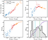 |
Fig. 1. Top-left panel: CF275W, F336W, F814W vs mF275W − mF438W pseudo two-colour diagram of the HB stars in NGC 6752. Stars with T < 11 500 K, T > 18 000 K, and 11 500 K < T < 18 000 K are marked with orange, blue, and red points. Top-right panel: mF275W vs mF275W − mF814W CMD of the HB stars in NCG 6752. Bottom-right panel: Histogram of the colour distribution of the photometric data. The purple profile represents the cumulative distribution of the points. The two dashed lines, green and cyan, mark the position of the G- and M- jumps, respectively. Bottom-left panel: mF438W vs mF438W − mF814W CMD of the HB stars in NCG 6752. Where applicable, we plotted the stars in the three ranges of temperature with the same colour coding. |
2.3. Models
We adopted the stellar-evolution models and the isochrones from T20 and T21. The models themselves were obtained with the ATON 2.0 stellar evolution code by Ventura et al. (1998) and Mazzitelli et al. (1999). The models span a broad range of [Fe/H], [α/Fe] and Y values to accommodate the variations observed among the Galactic GC population. The individual HB tracks were followed until they reached Hec ⇐ 0.01 (i.e. right before the proper end of the core helium burning).
We compared the photometric data of NGC 6752 and NGC 2808 with grids of synthetic CMDs derived from the appropriate models. The individual simulations in our grids were calculated following the recipes of D’Antona et al. (2005, along with the references therein), including a number of HB stars (2000) large enough to avoid any variance problem. The mass of each HB star (MHB) is chosen as follows: MHB = MTip(Z, Y, A)−ΔM(μ, δ), where MTip is the stellar mass at the RGB tip, function of age (A), metallicity (Z), and helium content (Y), while ΔM is the mass lost by the star, described by a Gaussian profile with central value, μ, and standard deviation, δ, which will be our sought of average integrate mass loss and its spread3. Finally, we simulated the effect of metal levitation between the Grundahl et al. (1999) and Momany et al. (2012) jumps by using a super-solar bolometric correction when the stars reach appropriate temperatures, as suggested in the results of Grundahl et al. (1999), Dalessandro et al. (2011), Brown et al. (2016), Tailo et al. (2017).
3. The HB of NGC 6752
In this section, we describe the analysis of the HB in NGC 6752, starting from its morphology (Sect. 3.1) and then analysing its stellar populations. We start from the two extreme ones (the 1G and the 2Ge; Sect. 3.2) and then we present our modelling of the intermediate branch (Sect. 3.3).
3.1. Morphology
Our sample for this cluster consists of 115 HB stars, which all populate the part of the branch bluer of the instability strip (IS). Milone et al. (2014) found a value of ∼0.38 mag for the parameter L14 and if we follow the separation introduced in T20, we can describe NGC 6752 as a M13-like cluster5. Composed of blue stars only, this particular HB is best studied with combinations of optical and UV filters, as we show in Fig. 1.
Two important discontinuities are observed along the HB of every GC and NGC 6752 is no exception: the Grundahl et al. (1999) and Momany et al. (2004) jumps are apparent (hereinafter, the G- and M-jumps). These are universal features of the HB locus, connected to changes of the internal structure of the HB stars with temperature6. The G-jump and the M-jump are located at ∼11 500 and ∼18 000 K (Grundahl et al. 1999; Momany et al. 2004; Brown et al. 2016, 2017), respectively. As Brown and their collaborators have shown, they are most easily identified in the CF275W, F336W, F438W7 versus mF275W − mF438W diagram.
We show this diagram for NGC 6752 in the upper left panel of Fig. 1. Even if the HB in NGC 6752 is populated without apparent gaps and its metallicity value is low ([Fe/H] = −1.54), the transitions associated with the jumps can be appreciated by eye, in spite of their not being so sharp. Stars cooler than the G-jump are shown in orange, those hotter than the M-jump in blue, and the ones between the two in red. Therefore, we identified 32 stars before the 11 500 K mark and 39 stars in the region past 18 000 K. As a consequence, 41 stars have been found to populate the region between the two jumps. In the following, we use this separation to comment on the morphology of the HB of this cluster.
We report the mF275W versus mF275W − mF814W CMD in the upper right panel of Fig. 1. This is one of the best combinations of filters in the HST Treasury survey to study bHB stars, as it is the one with the largest sensitivity to temperature (Piotto et al. 2015; Milone et al. 2015, 2017, 2018). We also report the histogram of the colour distribution of the points (black) as well as their cumulative distribution (red) in the bottom right panel of Fig. 1. From the figure, we can see there that the distribution of the HB stars in NGC 6752 has one narrow peak at mF275W − mF814W ∼ −2.5, a group of stars broadly distributed at mF275W − mF814W ∼ −1, and a final peak at mF275W − mF814W ∼ 0. The cumulative distribution shows that the bluest peak hosts ∼20% of stars, the reddest one hosts ∼20% as well, while the majority (∼60%) of the HB stars are in the central group. With the separation in temperature we indicate in the upper left panel, we locate the position of the G-jump at mF275W − mF814W ∼ −0.45 and the M-jump at mF275W − mF814W ∼ −1.62 in the CMD. There seems to be no noticeable gaps at these locations in the HB. We also report the position of the jumps in the lower right panel of Fig. 1 as the green and purple dashed lines, respectively for the G- and M-jump. For completeness, we also plot the mF438W versus mF438W − mF814W CMD in the lower right panel of Fig. 1. In this CMD the locations of the G and M jumps are mF438W − mF814W ∼ −0.03 and −0.19, respectively. This procedure ensures that all the peaks in the colour distribution are independent from the G- and M-jump positions and allows us to associate the peaks with the three observed stellar populations.
3.2. Mass loss of the first and the extreme second generation stars
We refer to the results from T20 with respect to the 1G on the HB of NGC 6752; however, since the assumptions we make here for the 2Ge are slightly different from the ones we made in our past work, to ensure consistency, we studied these stars again. For the 1G, its colour distribution is best-fit by a mean mass loss value of μ = 0.216 ± 0.022 M⊙ and mass-loss spread value of δ = 0.006 ± 0.001 M⊙. We used these values to identify and study the 1G stars on the branch.
The 1G simulation corresponding to the selected parameters is reported as the red contour plot in the upper panel of Fig. 2, while the solid red points represent a typical realisation of the simulation. To find which stars belong to the 1G, we used the best fit simulation and calculated its 2D kernel density estimation (KDE, the red contour lines) to obtain its value at the location of each of the 115 stars in the sample. Then, we tentatively identified the stars in the 1G population as those that have a KDE values that significantly differs from zero; namely, values greater than 5% of its maximum value, highlighting them as solid, dark grey points in Fig. 2.
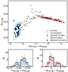 |
Fig. 2. Best-fit simulations for the 1G and 2Ge stars in NGC 6752. The grey and black points are the stars belonging to the 1G and the 2Ge, respectively, selected according to the simulation area (red and blue, respectively, for the 1G and the 2Ge). The coloured points, colour-coded in the same way as the simulations, are a typical realisation of each population. Histograms in the bottom panels compare the colour distribution of the two simulations (red and blue) and the selected stars (black). The simulation histograms are normalized to the number of stars included in each population. |
We found that 37 ± 5 stars belong to the 1G, corresponding to ∼32.2 ± 4.2%, in good agreement with both Milone et al. (2013, 2017). The error on these numbers has been estimated via a bootstrapping procedure8. For completeness, the histograms in the bottom right panel of Fig. 2 directly compare the colour distribution of the selected 1G stars with the simulated ones; the red histogram is normalised at the same number of stars in the selected sample.
Finally, to provide a more detailed view of this result, we plot the selected 1G stars together with the other stellar populations along the HB of NGC 6752 in Fig. 3. In the figure, the 1G stars we previously identified are plotted as the red open points, together with the zero-age horizontal branch (ZAHB) loci of appropriate chemistry (top panel) and the stellar models describing their post ZAHB and post HB evolution (bottom panel). The solid coloured diamonds in the figure highlight the position of the end of the core helium burning.
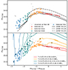 |
Fig. 3. Top panel: mF275W vs mF275W − mF814W CMD of the HB in NGC 6752. Each population is highlighted with the same colour code used in other part of this paper. The three lines represents the ZAHB loci of appropriate metallicity and Y = 0.25, 0.28, 0.35, respectively for the solid, dashed, and dot-dashed one. Bottom panel: Same as the top panel, but we show the stellar tracks involved in the simulations to show their evolution during and past core helium burning. For each track, the end of the core helium burning is highlighted by the coloured, solid diamonds. Tracks are coloured as their respective stellar populations. |
To study the 2Ge, we applied the technique from T20 using the helium mass fraction for the bluest MS provided by Milone et al. (2013). In summary, we calculated the grids of simulated HBs with different parameters, compared them with the photometric data, and chose, as the best fit, the simulation minimizing the chi-squared distance (hereinafter χd2) between the colour histograms of the data and the simulated stars. In this case, our algorithm was set to look for the simulation that best matches the bluest group of stars on the HB.
For the 2Ge of NGC 6752, the grids have the parameters listed in Table 2. The comparison with the data yields that the best fit simulation is the one with μ = 0.285 ± 0.024 M⊙ and δ = 0.004 ± 0.002 M⊙. The errors on these values include different sources of uncertainties. As expected, this value is slightly larger than the one we found previously because here we adopted a slightly lower value of helium enhancement.
Parameters of the HB simulation grids used for NGC 6752.
The upper panel of Fig. 2 reports the comparison of the best fit simulation (blue contours) with the data and a typical realisation (solid blue points), while we report the comparison between the colour histograms of the simulation with the selected stars (represented as solid black points in the top panel of the figure) in the lower left panel. The identification is performed in the same way as the 1G case. We identified 24 ± 4 stars as 2Ge, representing the ∼20.9 ± 3% of all stars in the branch. As in the case of the 1G stars, the errors have been estimated via bootstrapping.
As in the case of the 1G, we plot the selected 2Ge stars and the models involved as the open blue points and tracks in Fig. 3. We find it worth noting that, as shown by the models in the figure, the three stars at mF275W ∼ 14.5 and mF275W − mF814W ∼ −2.6 are compatible with being in the post-HB evolutionary phase and should be included in this population, bringing the total number of stars in it to 27 (∼23.5%). We report the main parameters of these two populations in Table 3.
Parameters of the HB population in NGC 6752.
3.3. Mass loss of the intermediate second generation stars
Here, we discuss how we interpret and simulate the stars in the intermediate HB (iHB) and its stellar populations.
First, we removed stars that have been previously identified as 1G and 2Ge from the CMD. Then, we tried to simulate this part of the branch with a single stellar population (see Sect. 2). We built the appropriate grids (see Table 2) and looked for the best fit. Our procedure identifies the minimum of the χd2 distribution at μ = 0.246 M⊙ and δ = 0.017 M⊙. However, the problem with this result is that, even upon visual inspection, the selected simulation is not a good fit because it does not adequately describe the peaks we see in the colour distribution of the stars, as demonstrated by the plot in the bottom panel of Fig. 4. Therefore, we must make an additional assumption.
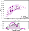 |
Fig. 4. Contour plot and typical realisation of the best fit simulation for the intermediate stellar population in NGC 6752. The histograms in the bottom panel compare the colour distributions of both; the magenta one is normalised to the total number of stars in the plot. |
Milone et al. (2013) used a combination of UV and optical filters, while Milone et al. (2019) used infrared bands to show that the intermediate MS is clearly broadened compared to the others, down to the low mass regime, as seen in the IR. This has been interpreted in both occasions as a sign of mixed populations. Following on this, it is straightforward to imagine the intermediate HB stellar populations as being composed of (at least) two sub-populations, which we name 2G1a and 2G1b; their helium values are slightly different, but the average is compatible with the value estimated by Milone et al. (2013). Thus, we associate Y = 0.255 and to the 2G1b Y = 0.270 the 2G1a. These values, once averaged using the population ratio found in both Milone et al. (2013, 2019), give back the average helium abundance for the intermediate stellar population in NGC 67529.
We went on to associate the reddest group of stars of this part of the HB with the 2G1a. We calculated synthetic HB grids with the appropriate parameters (see Table 2) and looked for the best fit, which was determined to be at μ = 0.246 ± 0.020 M⊙ and δ = 0.007 ± 0.002 M⊙. This simulation is the one represented as the orange contours and solid coloured points in the upper panel of Fig. 5. Using the 2D KDE obtained from the best fit simulation, we associate 37 ± 5 stars with this group, giving us a population ratio of 32.2 ± 4.3%. The selected stars are represented as solid dark grey points in Fig. 5, together with a sample realisation of the simulation.
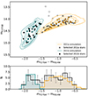 |
Fig. 5. Same as Fig. 2 but for the case where the intermediate HB in NGC 6752 is described with two individual stellar populations. |
To study the bluest part of the intermediate branch, which we dub 2G1b, we used the simulation grid described in Table 2. We find that the best fit simulation10 is the one with μ = 0.270 ± 0.021 M⊙ and δ = 0.005 ± 0.002 M⊙. This simulation is represented by the teal contour plot and points in the main panel of Fig. 5. We associate 17 ± 3.6 stars with the 2G1b, representing 14.78 ± 3.1% of the total stars in the sample.
Collectively, the two populations host ∼46 ± 5.3% of the total stars on the HB. Furthermore the output average helium abundance of this intermediate population is 0.258. Both values are in good agreement with the results from Milone et al. (2013). A direct comparison of the histograms of the two best fit simulations and the data is reported in the bottom right panel of Fig. 5, which offers a better description than the single population case. Finally, it is worth noting that in this CMD, there is a group of stars compatible with being part of the post-HB of the 2G2 stars, located at mF275W ∼ 14.0 − 13.5, mF275W − mF814W ∼ −1.2. Furthermore, the lone star at mF275W ∼ 14.25 − 14.0, mF275W − mF814W ∼ 0.25 can be associated with the post HB phase of the 2G1. This is shown by the HB tracks plotted in the bottom panel of Fig. 3. The main parameters of these two populations are reported in Table 3.
4. The HB of NGC 2808
In this section, we discuss the detailed analysis of the HB in NGC 2808. Initially, we illustrate its morphology (Sect. 4.1). Afterwards, we discuss the populations found in the rHB (Sect. 4.2) and then the ones populating its bHB (Sect. 4.3).
4.1. Morphology
Figure 6 illustrates the morphology of the HB in NGC 2808 in optical and UV filters. The HB in this cluster hosts 839 stars populating a broad range of colour values and separated into easily identifiable groups, as seen in the CMDs plotted in Fig. 6. Milone et al. (2014) found a value of ∼0.094 mag for the parameter L1. This classifies NGC 2808 as M3-like (as in T20). The IS is easily identifiable in all the diagrams; thus, we find that the rHB hosts 362 stars (∼43% of the total), whereas the bHB hosts 465 stars (∼53%).
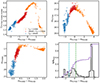 |
Fig. 6. Top-left panel: CF275W, F336W, F814W vs mF275W − mF438W pseudo-CMD of the HB stars in NGC 2808. The stars with T < 11 500 K, T > 18 000 K, and 11 500 K < T < 18 000 K are marked with orange, blue, and red points to show the location of the G- and M- jumps. Top right panel: mF275W vs mF275W − mF814W CMD of the HB stars in NCG 2808. Bottom-right panel: Histogram of the colour distribution of the photometric data. The cumulative distribution of the points is plotted as the purple profile. The dashed lines in the panel, green and cyan, represent the position in mF275W − mF438W of the G- and M- jumps, respectively. Bottom-right panel: mF438W vs mF438W − mF814W CMD of the HB stars in NCG 2808. The colour coding of the points highlight the temperature ranges of the stars where applicable. |
The upper left panel of Fig. 6 reports the CF275W, F336W, F438W versus mF275W − mF438W diagram for this cluster. As expected, due to the higher metallicity, the discontinuities on the HB are more evident compared to the NGC 6752 case. We identify ∼580 stars (∼57%, orange) before the G-Jump and ∼170 stars (∼17%, blue) after the M-jump. Consequently, we find that ∼260 (∼26%, red) stars populate the region between the two jumps.
We report the identification of these three ranges of temperature in the other CMDs in Fig. 6. More specifically, by looking at the mF275W − mF814W CMD (top-right panel in Fig. 6), we see that the position of the G-jump is at mF275W − mF814W ∼ 0.24 and the M-jump is located at mF275W − mF814W ∼ −1.16. To better describe the morphology of this HB, we report (in the bottom right panel of Fig. 6), the mF275W − mF814W histogram for these HB stars (black) and their cumulative distribution (red). The distribution of stars along the branch has four major peaks. From the left, the first two are in the blue at mF275W − mF814W ∼ −2.12 and ∼−1.48 respectively; they collectively host ∼18% of the stars in the branch. A third, broader peak is seen at mF275W − mF814W ∼ −0.29 and hosts ∼35% of stars. Finally, the highest peak is at mF275W − mF814W = 3.5, hosting ∼47% of the stars in the HB. In addition the colour location of the two jumps is reported as the green and purple dashed lines, respectively, for the G- and M-jumps. We see that, as in the case of NGC 6752, for the G-jump, no gaps are present at the location of the jumps, reinforcing their independence from the MPs phenomenon.
For completeness, we also report the mF438W versus mF438W − mF814W optical CMD in the lower left panel of Fig. 6. Similar considerations to those we made for the mF275W − mF814W case can also be made here. We proceeded to study the stellar populations found in this HB, starting from the red side.
4.2. Mass loss of the stellar populations in the red HB
The rHB of NGC 2808 is more complex than the one found in NGC 6752. Indeed, while the latter hosts one population, the results from Marino et al. (2014) show that the former is composed of a mixture of two stellar populations, one more sodium-poor than the other (see their Fig. 11). Combining this results with other spectroscopic and spectro-photometric analysis (see e.g. Carretta et al. 2009, 2018; Milone et al. 2015; Marino et al. 2017, and references therein), it is clear how the low-sodium population is the 1G, accounting for Population A and B, while the high sodium population is part of the least enhanced part of the 2G, accounting for Population C, dubbed ‘2G1’. This is also corroborated by the information contained in the cumulative distribution of the HB stars plotted in Fig. 6, as we see there that the rHB contains roughly 47% of stars, corresponding to the sum of the A, B, and C populations.
Therefore, in this more complex scenario, our method would provide unreliable results because there are mixed populations in the rHB. Milone et al. (2012b) and Dondoglio et al. (2021) showed that in clusters with cool-enough rHB stars, a special combination of filters is able to separate the stellar population found there. In the case of NGC 2808, the stars in the rHB are too hot to be effectively separated. Thus, we use the spectroscopic results from Marino et al. (2014) and the cross-matching they performed with the ground based photometric catalogue from Momany et al. (2004). Our procedure and results are summarised in Fig. 7.
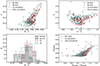 |
Fig. 7. Top-left panel: Colour magnitude diagram in the V vs B − V plane of the photometric data of the HB stars in NGC 2808 from Momany et al. (2004). The Na-Poor and Na-Rich populations from Marino et al. (2014) are represented with filled and open points, respectively. The red and teal contours and points represent the best fit simulations for the 1G and the 2G1 in this cluster, respectively, together with a sample realisation. Bottom-left panel: Histograms of the colour distribution of the stars belonging to the two populations in the data and in the best fit simulations. The histograms of the simulated stars are normalised to the same number of stars we see in the observed sample. Top-right panel: Same as the top left panel, but for the U vs U − V CMD. Bottom-right panel: Contour plot of the best fit simulation for the 1G and 2G1 populations compared with the mF606W vs mF438W − mF606W CMD for the HST photometric catalogue. |
We produced adequate simulation grids (see Table 4) and compared them with the data to find the best-fit simulations. We find that the best fit for the 1G is located at μ = 0.110 ± 0.024 M⊙ and δ = 0.009 ± 0.003 M⊙, while for the 2G1, the best-fit values are μ = 0.126 ± 0.023 M⊙ and δ = 0.011 ± 0.003 M⊙11. We report the best fit simulation as the red and teal contour plots, respectively for the 1G and the 2G1, in the panels of Fig. 7. To also show the fit qualitatively, in the lower left panel of Fig. 7 we report and compare the histograms of the B − V colour distributions for the two populations of stars (as labelled), with their best-fit simulations, plotted with the same colour coding adopted for the contour plot in the upper left panel. As in other similar instances throughout this work, the series of solid coloured points represent a sample realisation of the simulations. For completeness, the two right panels in Fig. 7 reproduce the U versus U − V (top) and mF606W versus mF438W − mF606W CMDs (bottom) to show how the best-fit simulations appear in those planes and bands. As in previous cases, all the relevant parameters of the simulated populations are summarized in Table 5.
Parameters of the HB simulation grids used for NGC 2808.
Parameters of the HB population in NGC 2808.
Finally we plot the tracks involved in this simulation, together with the ZAHBs of appropriate chemistry, in Fig. 8. In this figure, we also plot the mF275W versus mF275W − mF814W CMD, highlighting the selected stars in each populations. We note that for the 1G and the 2G1, this means highlighting the entirety of the rHB, as we have no means (for now) to separate the population in the HST bands.
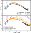 |
Fig. 8. Top panel: mF275W vs mF275W − mF814W CMD of the HB in NGC 2808. Each population we identify is highlighted with the same colour code used in other part of this work. The three lines represent the ZAHB loci of appropriate as in Fig. 3. Bottom panel: Same as the top panel, but with the stellar tracks involved in the simulation. |
4.3. Mass loss of the stellar populations in the blue HB
In this section, we discuss the parameters of the stellar populations hosted in the bHB of NGC 2808. The bHB is the part of the HB located at bluer colour than the IS. In the case of NGC 2808, it can be divided into two other sections: an iHB, located right after the IS and around the knee of the HB in Fig. 6, and the eHB, hosting the two bluest groups of stars in the branch. We discuss the iHB first and then explore the more complex case of the eHB.
4.3.1. The iHB
The iHB in NGC 2808 is the part of the HB that starts immediately after the blue side of the IS. From the cumulative distribution reported in Fig. 6, we see that this section of the branch hosts ∼35% of the HB stars. The G-jump is located in this section of the HB (see Fig. 6) but it does not correspond to an actual gap, as the distribution of the stars is continuous both in the mF275W versus mF275W − mF814W and mF438W versus mF438W − mF814W CMDs, proving again that the G- and M-jumps are not connected to the presence of different stellar populations.
From the numerical considerations, stemming from the results in Milone et al. (2015) and the spectroscopic indication from Marino et al. (2014), we can assign this group of stars to Population D. Then, to find the parameters and the extension of this population on the branch, we can apply the same method we used in the rest of this work. We compared an adequate grid of simulations (see Table 4) with the data and found that the simulation minimizing χd2 is the one with μ = 0.203 ± 0.023 M⊙ and δ = 0.027 ± 0.003 M⊙.
As in other instances presented here, we assigned stars that have a KDE significantly different from zero to this population, finding that the 2G2 hosts 294 ± 15 stars. A direct comparison of the simulation and the data is represented via the CMD and the histograms in Figs. 8 and 9. In the latter, we also show the tracks involved in the simulation and the post HB evolution predicted for these stars. Therefore, the few stars located at mF275W ∼ 16.5, and the ones at mF275W − mF814W ∼ 2, mF275W ∼ 17.0 are compatible to be stars in the post-HB phase. All other relevant parameters are summarized in Table 5.
4.3.2. The eHB
The last part of the HB in NGC 2808, usually referred to eHB, hosts about ∼20% of the total number of HB stars, in two groups of stars that are well separated in colour. The hottest blue tail, dubbed blue hook (bhk Moehler et al. 2004) has generally been interpreted as a group of stars suffering an extreme helium flash. The study of the eHB of NGC 2808 will result in a more complex picture than previously found in the literature and its complexity could bear some consequences on the proposed model of pre-MS early disk loss.
Lee et al. (2005) and D’Antona & Caloi (2008) first showed that the UV magnitudes and colours of the bhk could only be fit with models having a very high helium abundance in the envelope. D’Antona & Caloi (2008) later proposed that the eHB and the bhk belonged to the same high helium population responsible for the presence of the bluest MS in NGC 2808. The lowest masses in this group would undergo the late helium flash, with flash-induced mixing (e.g. Castellani & Castellani 1993; Sweigart 1997; Brown et al. 2001; Cassisi et al. 2003 or Tailo et al. 2015 and references therein) and burn helium in the core at the bhk location. Based on this hypothesis, and in the absence of extensive computations following the He–core flash and the flash mixing event, they could parametrize the limiting mass between the standard flash and the flash-mixing in order to describe the eHB and the bhk as a single group. This interpretation was indeed guided by the recent (at the time) determination of the triple MS (D’Antona et al. 2005; Piotto et al. 2007) in this cluster.
These steps allowed us to go on and make use of our new stellar models, which include the flash–mixing explicitly computed in Tailo et al. (2015) and T20. For Y = 0.35, the standard evolution extends down to a mass of M = 0.475 M⊙, while the smallest mass that can populate the EHB is M ∼ 0.49 M⊙. Thus, there is a mass range 0.475 < M/M⊙ < 0.490, which is not present in the data, but would result in the eHB distribution if we adopt a single helium content and a continuous mass-loss distribution for the two groups of stars (see Fig. 10). Thus, our interpretation of the hot end of the HB in NGC 2808 needs to become more complicated than in previous approaches12.
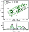 |
Fig. 10. Same as Fig. 2, but for the case of the eHB in NGC 2808 simulated as an individual group of stars. The dashed and the dot-dashed lines represent the canonical ZAHB of appropriate metallicity with Y = 0.28 and Y = 0.35, respectively. We also report the end of the canonical HB at the bottom. |
A first possibility is that Population E is actually composed of two sub-populations (dubbed 2Gea and 2Geb). Their average helium values includes that estimated by Milone et al. (2015, namely, 0.34). They populate the two clumps observed in the eHB (the EBT1 and EBT2, Bedin et al. 2000). This interpretation is corroborated by the results by Milone et al. (2012c). In their study, Milone and collaborators found that the bluest MS in NGC 2808 has a higher colour dispersion. This larger spread may indicate, as in the case of NGC 6752, the presence of more than one stellar population with helium values close enough to merge but also different enough to populate different part of the HB. Hence, we needed to make an additional assumption and assign helium abundance values to these two sub populations. Thus, we assigned Y = 0.33 and Y = 0.36, respectively, for 2Gea and the 2Geb. The two groups host more or less the same number of stars and these two values return the result of Y = 0.34 found by Milone et al. (2015), once they are averaged. In this description, the latter of the two groups undergoes the process of late-flash mixing and popoulates the bhk. We produced two simulation grids that differ only in helium content (see Table 4) and compared them with the data, finding that the red side of the eHB (hosting the 2Gea) is best fit by the simulation with Y = 0.33, μ = 0.226 ± 0.025 M⊙, and δ = 0.004 ± 0.001 M⊙; on the other hand, the bluest group (identified here as 2Geb) is best described by the simulation with Y = 0.36, μ = 0.236 ± 0.024 M⊙, and δ = 0.008 ± 0.002 M⊙. The results are described in Fig. 11, where we plot the two simulations with magenta and blue contour lines, respectively, for 2Gea and the 2Geb. With the same method used earlier in this work, we found 47 ± 6.9 and 53 ± 7.9 stars. For completeness, the comparison of the histograms is reported in the bottom panels, following the same colour coding of the contour plots. The other relevant parameters of these populations are summarized in Table 5.
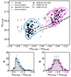 |
Fig. 11. Same as Fig. 2, but for the case of the eHB in NGC 2808. Dashed and the dot-dashed lines represent the canonical ZAHB of appropriate metallicity with Y = 0.28 and Y = 0.35, respectively. |
An alternative description of the eHB in this cluster can be obtained if we consider the two groups as part of a single population. In this description both groups have the same Y and suffered different amounts of total mass loss and the group that suffered the most populated the bhk (as suggested by the Tailo et al. 2015 scenario for the bhk in ω Centauri). To obtain this description, we compared the two parts of the eHB with a grid of model HBs having Y = 0.34 and the same range of μ and δ from the previous case. The simulations that best fit the two groups are the ones corresponding to μ = 0.213 ± 0.021 M⊙, with δ = 0.005 ± 0.001 M⊙, and μ = 0.256 ± 0.024 M⊙ with δ = 0.008 ± 0.002 M⊙, respectively for the 2Gea and 2Geb. The other parameters of these two stellar populations are summarized in Tables 4 and 5. It is worth noting that our late flash model for the most enhanced chemistry has a mass of ∼0.46 M⊙, while the value of μ of the best fit simulation gives a lower average mass: this implies that the peak of the mass loss for this population is in an interval that mainly produces helium white dwarfs. This may explain some of the missing AGB stars noted in Marino et al. (2017). This is in agreement with our previous fidngs about ω Cen and NGC 2419 (Di Criscienzo et al. 2015; Tailo et al. 2015). From the track plotted in the lower panel of Fig. 8, we se that the stars located at mF275W − mF814W < −1.5 and mF275W − mF814W < −2.2 are compatible with their being post-helium-burning stars, corresponding the two parts of the eHB.
5. Discussion
In this work, we have analysed the stellar populations found along the HB of NGC 6752 and NGC 2808, while breaking the traditional parameter degeneracy associated with these stars, using helium abundance estimates from the literature (see Sect. 2). Our findings suggest that the total, integrated mass loss suffered by these stars during the ascent of the RGB needs to be significantly increased in the stellar populations past the 1G.
More specifically, in NGC 6752, the minimum mass loss associated with the 1G is 0.216 M⊙ while the maximum value for the mass loss is 0.285 M⊙ for the 2Ge. Our values of μ and  are in agreement (within their errors) with the ones in Cassisi et al. (2014). In NGC 2808, the minimum mass loss, associated with the 1G, is 0.113 M⊙, while the maximum value of the mass loss is 0.226 M⊙ or 0.256 M⊙, depending on the description adopted to describe the eHB in that cluster. Therefore, a non-negligible increase in mass loss is necessary to describe each stellar population on the HB. The exact value of the needed increase is reported in Tables 3 and 5. The errors reported in the table have been obtained with the method from Tailo et al. (2020).
Figure 12 reports the increase of mass loss (Δμ) versus the helium enhancement (δY) of the stellar populations analysed in this paper. The red diamonds are for the stellar populations in NGC 6752 and the blue triangles are for the NGC 2808 ones. The two blue squares are for the alternative description of NGC 2808 eHB that we provide in Sect. 4.3.2. In the figure, we also plot the data for the 2Ge from T20 as grey, semi-transparent points. We clearly see that all the analysed stellar populations describe a clear δμ versus δY relation, compatible with the one described by the points from T20. In other words, we find that the populations having ‘intermediate’ helium abundances in the two clusters examined here display a similar behaviour to the populations with similar helium abundances in many other clusters.
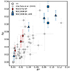 |
Fig. 12. Mass-loss increase (Δμ) vs helium enhancement (ΔY) of the stellar populations studied in this work. The two series of points refer to the stellar populations (SP) in NGC 6752 (red diamonds) and NGC 2808 (blue triangles). The two blue squares in the figure refer to the alternate description of the eHB in NGC 2808. In the figure, the data from Tailo et al. (2020) are also reported. |
This finding reinforces the tentative explanation advanced in T20 (see their Fig. 18) to explain the results, namely, that the increase in mass loss is the consequence of the physical environment in which populations with different helium formed. In the context of the standard ‘AGB model’, 2Ge forms at higher density than 1G, in the very compact core of the GC, where the pure winds of the massive AGBs are gathered, with the maximum values of δY (D’Ercole et al. 2008). The intermediate populations form, instead, by a mixing of the AGB ejecta with re–accreting pristine gas, resulting in intermediate values of Y. Also, they form in a lower density environment than the 2Ge, as confirmed in the hydrodynamical simulations from Calura et al. (2019). The denser the environment, the earlier the destruction of the protostellar accretion disk will be: this will lock the stellar rotation with the disk rotation at higher velocities and make the acceleration of the stellar rotation more effective due to the conservation of angular momentum in the contracting pre-MS star. If the early higher rotation rate implies a larger average mass loss rate, the observed relation of Fig. 12 can be naturally explained as the fossil trace of the formation mechanism.
One complication seen in our results is the ambiguous way in which we have reproduced the eHB plus bhk stars in NGC 280813. If we trust the models, these two groups have either a difference in helium content or a difference in mass loss. The different helium content indicated by ΔY ∼ 0.02 could imply an inhomogeneity in the helium content of the stars forming from the pure ejecta of the most massive AGBs or super-AGBs and requires a careful investigation of the AGB model results. An abrupt difference in the mass loss rate could be explained if the birth location of the stars within the cooling flow would have a further effect on early disk loss.
6. Summary
In the present work, we combined high-precision photometry from the UV Legacy survey (Piotto et al. 2015; Nardiello et al. 2018) of NGC 6752 and NGC 2808, with stellar population models to characterize the intermediate stellar populations hosted in their HB. To constrain the helium abundance in each stellar population, we used the helium abundances inferred by Milone et al. (2013, for NGC 6752) and Milone et al. (2015, for NGC 2808). The analysis of the HB population was carried out following the method developed by T20 and T21. We summarized the parameters we derived for each stellar populations in Table 3. Our main results can be summarized as follows:
-
(i)
In NGC 6752, we divided the HB into four different stellar populations. The values of integrated mass loss we found in our study range from 0.216 M⊙ for the 1G (from Tailo et al. 2020) to 0.280 M⊙ for the 2Ge. The other two intermediate populations have values of mass loss located in between these two: 0.246 M⊙ for the 2G1 and 0.270 M⊙ for the 2G2. We report all the details of these stellar populations in Table 3.
-
(ii)
In NGC 2808, the description is more complex. We identified five stellar populations and the integrated mass loss our algorithm associated with each of them varies from 0.113 M⊙, for the 1G to 0.236 M⊙ (or 0.256 M⊙ depending on the description adopted) for the 2Ge, populating the bhk of the HB. For the other intermediate populations, corresponding to the different sub populations of the 2G, we found integrated mass loss values of 0.126 M⊙, 0.203 M⊙, and 0.226 M⊙, as detailed in Table 5.
Our combined results show that the amount of mass loss correlates with the helium content of the stellar populations. In particular, the pattern of increased mass loss is consistent with the behavior described in T20, which we interpret as the signature of the MP formation mechanism.
The nomenclature, here and in the following, follows T20, T21 and the other works from Milone and collaborators. 1G stands for the ‘first generation’, i.e. the population of stars that has chemical pattern compatible with the field stars of the same metallicity. In this context, 2G (second generation) collectively indicates the group of stellar populations with signatures of hot proton capture nucleosynthesis. Finally, 2Ge indicates the part of the 2G with the most altered chemistry in each cluster.
We use the Gaussian profile to the mass loss for it’s ease of use and consistency with the other paper works from our group, however other kind of shapes for the mass loss can work. See e.g. Cassisi et al. (2014) for a case where the modelling is done with a flat distribution.
More specifically, this refers to the changes of the two external convective layers and their interplay with radiative levitation, see Grundahl et al. (1999), Momany et al. (2004), Brown et al. (2016, 2017), Tailo et al. (2017) and references therein.
We note that these values are not meant to be conclusive determinations of the helium mass fraction of the intermediate stellar populations in NGC 6752, which is beyond the scope of this work. Rather, they are meant to serve as a guide to simulate the HB in this cluster to study the mass loss of its stellar populations. Indeed, similar considerations still hold with slightly different values of helium abundance, as long as the average helium abundance of the combined population is compatible with the estimate from Milone et al. (2013).
Acknowledgments
This work has been funded by the European Union – NextGenerationEU RRF M4C2 1.1 (PRIN 2022 2022MMEB9W: “Understanding the formation of globular clusters with their multiple stellar generations”, CUP C53D23001200006), and from the European Union’s Horizon 2020 research and innovation programme under the Marie Skłodowska-Curie Grant Agreement No. 101034319 and from the European Union – NextGenerationEU (beneficiary: T. Ziliotto). SJ acknowledges support from the NRF of Korea (2022R1A2C3002992, 2022R1A6A1A03053472).
References
- Armitage, P. J., & Clarke, C. J. 1996, MNRAS, 280, 458 [NASA ADS] [Google Scholar]
- Bastian, N., & Lardo, C. 2018, ARA&A, 56, 83 [Google Scholar]
- Baumgardt, H., & Hilker, M. 2018, MNRAS, 478, 1520 [Google Scholar]
- Baumgardt, H., Hilker, M., Sollima, A., & Bellini, A. 2019, MNRAS, 482, 5138 [Google Scholar]
- Bedin, L. R., Piotto, G., Zoccali, M., et al. 2000, A&A, 363, 159 [Google Scholar]
- Bouvier, J., Forestini, M., & Allain, S. 1997, A&A, 326, 1023 [NASA ADS] [Google Scholar]
- Brown, T. M., Sweigart, A. V., Lanz, T., Landsman, W. B., & Hubeny, I. 2001, ApJ, 562, 368 [NASA ADS] [CrossRef] [Google Scholar]
- Brown, T. M., Cassisi, S., D’Antona, F., et al. 2016, ApJ, 822, 44 [NASA ADS] [CrossRef] [Google Scholar]
- Brown, T. M., Taylor, J. M., Cassisi, S., et al. 2017, ApJ, 851, 118 [NASA ADS] [CrossRef] [Google Scholar]
- Calura, F., D’Ercole, A., Vesperini, E., Vanzella, E., & Sollima, A. 2019, MNRAS, 489, 3269 [Google Scholar]
- Carretta, E. 2015, ApJ, 810, 148 [Google Scholar]
- Carretta, E., Bragaglia, A., Gratton, R., & Lucatello, S. 2009, A&A, 505, 139 [NASA ADS] [CrossRef] [EDP Sciences] [Google Scholar]
- Carretta, E., Bragaglia, A., Gratton, R. G., et al. 2010, A&A, 516, A55 [NASA ADS] [CrossRef] [EDP Sciences] [Google Scholar]
- Carretta, E., Lucatello, S., Gratton, R. G., Bragaglia, A., & D’Orazi, V. 2011, A&A, 533, A69 [NASA ADS] [CrossRef] [EDP Sciences] [Google Scholar]
- Carretta, E., Bragaglia, A., Lucatello, S., et al. 2018, A&A, 615, A17 [NASA ADS] [CrossRef] [EDP Sciences] [Google Scholar]
- Cassisi, S., Schlattl, H., Salaris, M., & Weiss, A. 2003, ApJ, 582, L43 [NASA ADS] [CrossRef] [Google Scholar]
- Cassisi, S., Salaris, M., Pietrinferni, A., Vink, J. S., & Monelli, M. 2014, A&A, 571, A81 [NASA ADS] [CrossRef] [EDP Sciences] [Google Scholar]
- Castellani, M., & Castellani, V. 1993, ApJ, 407, 649 [NASA ADS] [CrossRef] [Google Scholar]
- Catelan, M., Borissova, J., Sweigart, A. V., & Spassova, N. 1998, ApJ, 494, 265 [Google Scholar]
- Dalessandro, E., Salaris, M., Ferraro, F. R., et al. 2011, MNRAS, 410, 694 [NASA ADS] [CrossRef] [Google Scholar]
- Dalessandro, E., Salaris, M., Ferraro, F. R., Mucciarelli, A., & Cassisi, S. 2013, MNRAS, 430, 459 [NASA ADS] [CrossRef] [Google Scholar]
- D’Antona, F., & Caloi, V. 2008, MNRAS, 390, 693 [CrossRef] [Google Scholar]
- D’Antona, F., Caloi, V., Montalbán, J., Ventura, P., & Gratton, R. 2002, A&A, 395, 69 [CrossRef] [EDP Sciences] [Google Scholar]
- D’Antona, F., Bellazzini, M., Caloi, V., et al. 2005, ApJ, 631, 868 [Google Scholar]
- D’Ercole, A., Vesperini, E., D’Antona, F., McMillan, S. L. W., & Recchi, S. 2008, MNRAS, 391, 825 [CrossRef] [Google Scholar]
- Di Criscienzo, M., Tailo, M., Milone, A. P., et al. 2015, MNRAS, 446, 1469 [NASA ADS] [CrossRef] [Google Scholar]
- Dondoglio, E., Milone, A. P., Lagioia, E. P., et al. 2021, ApJ, 906, 76 [NASA ADS] [CrossRef] [Google Scholar]
- Dotter, A., Sarajedini, A., Anderson, J., et al. 2010, ApJ, 708, 698 [Google Scholar]
- Dotter, A., Sarajedini, A., & Anderson, J. 2011, ApJ, 738, 74 [NASA ADS] [CrossRef] [Google Scholar]
- Faulkner, J. 1966, ApJ, 144, 978 [NASA ADS] [CrossRef] [Google Scholar]
- Fusi Pecci, F., & Bellazzini, M. 1997, in The Third Conference on Faint Blue Stars, eds. A. G. D. Philip, J. Liebert, R. Saffer, & D. S. Hayes, 255 [Google Scholar]
- Fusi Pecci, F., Ferraro, F. R., Bellazzini, M., et al. 1993, AJ, 105, 1145 [Google Scholar]
- Gratton, R., Bragaglia, A., Carretta, E., et al. 2019, A&ARv, 27, 8 [Google Scholar]
- Grundahl, F., Catelan, M., Landsman, W. B., Stetson, P. B., & Andersen, M. I. 1999, ApJ, 524, 242 [NASA ADS] [CrossRef] [Google Scholar]
- Härm, H., & Schwarzschild, M. 1964, ApJ, 139, 594 [Google Scholar]
- Harris, W. E. 1996, AJ, 112, 1487 [Google Scholar]
- Harris, W. E. 2010, ArXiv e-prints [arXiv:1012.3224] [Google Scholar]
- Iben, I., & Rood, R. T. 1970, ApJ, 161, 587 [Google Scholar]
- Lee, Y.-W., Joo, S.-J., Han, S.-I., et al. 2005, ApJ, 621, L57 [NASA ADS] [CrossRef] [Google Scholar]
- Legnardi, M. V., Milone, A. P., Armillotta, L., et al. 2022, MNRAS, 513, 735 [NASA ADS] [CrossRef] [Google Scholar]
- Marín-Franch, A., Aparicio, A., Piotto, G., et al. 2009, ApJ, 694, 1498 [Google Scholar]
- Marino, A. F., Milone, A. P., Piotto, G., et al. 2009, A&A, 505, 1099 [CrossRef] [EDP Sciences] [Google Scholar]
- Marino, A. F., Milone, A. P., Sneden, C., et al. 2012, A&A, 541, A15 [NASA ADS] [CrossRef] [EDP Sciences] [Google Scholar]
- Marino, A. F., Milone, A. P., Przybilla, N., et al. 2014, MNRAS, 437, 1609 [NASA ADS] [CrossRef] [Google Scholar]
- Marino, A. F., Milone, A. P., Yong, D., et al. 2017, ApJ, 843, 66 [NASA ADS] [CrossRef] [Google Scholar]
- Marino, A. F., Milone, A. P., Renzini, A., et al. 2019a, MNRAS, 487, 3815 [CrossRef] [Google Scholar]
- Marino, A. F., Milone, A. P., Sills, A., et al. 2019b, ApJ, 887, 91 [NASA ADS] [CrossRef] [Google Scholar]
- Mazzitelli, I., D’Antona, F., & Ventura, P. 1999, A&A, 348, 846 [NASA ADS] [Google Scholar]
- Milone, A. P., & Marino, A. F. 2022, Universe, 8, 359 [NASA ADS] [CrossRef] [Google Scholar]
- Milone, A. P., Piotto, G., Bedin, L. R., et al. 2012a, A&A, 540, A16 [NASA ADS] [CrossRef] [EDP Sciences] [Google Scholar]
- Milone, A. P., Piotto, G., Bedin, L. R., et al. 2012b, ApJ, 744, 58 [NASA ADS] [CrossRef] [Google Scholar]
- Milone, A. P., Piotto, G., Bedin, L. R., et al. 2012c, A&A, 537, A77 [NASA ADS] [CrossRef] [EDP Sciences] [Google Scholar]
- Milone, A. P., Marino, A. F., Piotto, G., et al. 2013, ApJ, 767, 120 [NASA ADS] [CrossRef] [Google Scholar]
- Milone, A. P., Marino, A. F., Dotter, A., et al. 2014, ApJ, 785, 21 [NASA ADS] [CrossRef] [Google Scholar]
- Milone, A. P., Marino, A. F., Piotto, G., et al. 2015, ApJ, 808, 51 [NASA ADS] [CrossRef] [Google Scholar]
- Milone, A. P., Piotto, G., Renzini, A., et al. 2017, MNRAS, 464, 3636 [Google Scholar]
- Milone, A. P., Marino, A. F., Renzini, A., et al. 2018, MNRAS, 481, 5098 [NASA ADS] [CrossRef] [Google Scholar]
- Milone, A. P., Marino, A. F., Bedin, L. R., et al. 2019, MNRAS, 484, 4046 [NASA ADS] [CrossRef] [Google Scholar]
- Moehler, S., Sweigart, A. V., Landsman, W. B., Hammer, N. J., & Dreizler, S. 2004, A&A, 415, 313 [NASA ADS] [CrossRef] [EDP Sciences] [Google Scholar]
- Momany, Y., Bedin, L. R., Cassisi, S., et al. 2004, A&A, 420, 605 [NASA ADS] [CrossRef] [EDP Sciences] [Google Scholar]
- Momany, Y., Saviane, I., Smette, A., et al. 2012, A&A, 537, A2 [NASA ADS] [CrossRef] [EDP Sciences] [Google Scholar]
- Nardiello, D., Libralato, M., Piotto, G., et al. 2018, MNRAS, 481, 3382 [NASA ADS] [CrossRef] [Google Scholar]
- Piotto, G., Bedin, L. R., Anderson, J., et al. 2007, ApJ, 661, L53 [NASA ADS] [CrossRef] [Google Scholar]
- Piotto, G., Milone, A. P., Bedin, L. R., et al. 2015, AJ, 149, 91 [Google Scholar]
- Renzini, A., D’Antona, F., Cassisi, S., et al. 2015, MNRAS, 454, 4197 [Google Scholar]
- Rood, R. T. 1970, ApJ, 161, 145 [Google Scholar]
- Salaris, M., Cassisi, S., & Pietrinferni, A. 2008, ApJ, 678, L25 [Google Scholar]
- Sandage, A., & Wildey, R. 1967, ApJ, 150, 469 [NASA ADS] [CrossRef] [Google Scholar]
- Schwarzschild, M., & Härm, R. 1962, ApJ, 136, 158 [Google Scholar]
- Sweigart, A. V. 1997, in The Third Conference on Faint Blue Stars, eds. A. G. D. Philip, J. Liebert, R. Saffer, & D. S. Hayes, 3 [Google Scholar]
- Tailo, M., D’Antona, F., Vesperini, E., et al. 2015, Nature, 523, 318 [Google Scholar]
- Tailo, M., D’Antona, F., Milone, A. P., et al. 2017, MNRAS, 465, 1046 [Google Scholar]
- Tailo, M., Milone, A. P., Lagioia, E. P., et al. 2020, MNRAS, 498, 5745 [CrossRef] [Google Scholar]
- Tailo, M., Milone, A. P., Lagioia, E. P., et al. 2021, MNRAS, 503, 694 [NASA ADS] [CrossRef] [Google Scholar]
- van den Bergh, S. 1967, AJ, 72, 70 [NASA ADS] [CrossRef] [Google Scholar]
- VandenBerg, D. A., Brogaard, K., Leaman, R., & Casagrande, L. 2013, ApJ, 775, 134 [Google Scholar]
- Ventura, P., Zeppieri, A., Mazzitelli, I., & D’Antona, F. 1998, A&A, 334, 953 [Google Scholar]
- Villanova, S., Geisler, D., & Piotto, G. 2010, ApJ, 722, L18 [NASA ADS] [CrossRef] [Google Scholar]
- Yong, D., Grundahl, F., Lambert, D. L., Nissen, P. E., & Shetrone, M. D. 2003, A&A, 402, 985 [NASA ADS] [CrossRef] [EDP Sciences] [Google Scholar]
- Yong, D., Grundahl, F., Nissen, P. E., Jensen, H. R., & Lambert, D. L. 2005, A&A, 438, 875 [NASA ADS] [CrossRef] [EDP Sciences] [Google Scholar]
- Yong, D., Grundahl, F., Johnson, J. A., & Asplund, M. 2008, ApJ, 684, 1159 [NASA ADS] [CrossRef] [Google Scholar]
All Tables
All Figures
|
Fig. 1. Top-left panel: CF275W, F336W, F814W vs mF275W − mF438W pseudo two-colour diagram of the HB stars in NGC 6752. Stars with T < 11 500 K, T > 18 000 K, and 11 500 K < T < 18 000 K are marked with orange, blue, and red points. Top-right panel: mF275W vs mF275W − mF814W CMD of the HB stars in NCG 6752. Bottom-right panel: Histogram of the colour distribution of the photometric data. The purple profile represents the cumulative distribution of the points. The two dashed lines, green and cyan, mark the position of the G- and M- jumps, respectively. Bottom-left panel: mF438W vs mF438W − mF814W CMD of the HB stars in NCG 6752. Where applicable, we plotted the stars in the three ranges of temperature with the same colour coding. |
| In the text | |
|
Fig. 2. Best-fit simulations for the 1G and 2Ge stars in NGC 6752. The grey and black points are the stars belonging to the 1G and the 2Ge, respectively, selected according to the simulation area (red and blue, respectively, for the 1G and the 2Ge). The coloured points, colour-coded in the same way as the simulations, are a typical realisation of each population. Histograms in the bottom panels compare the colour distribution of the two simulations (red and blue) and the selected stars (black). The simulation histograms are normalized to the number of stars included in each population. |
| In the text | |
|
Fig. 3. Top panel: mF275W vs mF275W − mF814W CMD of the HB in NGC 6752. Each population is highlighted with the same colour code used in other part of this paper. The three lines represents the ZAHB loci of appropriate metallicity and Y = 0.25, 0.28, 0.35, respectively for the solid, dashed, and dot-dashed one. Bottom panel: Same as the top panel, but we show the stellar tracks involved in the simulations to show their evolution during and past core helium burning. For each track, the end of the core helium burning is highlighted by the coloured, solid diamonds. Tracks are coloured as their respective stellar populations. |
| In the text | |
|
Fig. 4. Contour plot and typical realisation of the best fit simulation for the intermediate stellar population in NGC 6752. The histograms in the bottom panel compare the colour distributions of both; the magenta one is normalised to the total number of stars in the plot. |
| In the text | |
|
Fig. 5. Same as Fig. 2 but for the case where the intermediate HB in NGC 6752 is described with two individual stellar populations. |
| In the text | |
|
Fig. 6. Top-left panel: CF275W, F336W, F814W vs mF275W − mF438W pseudo-CMD of the HB stars in NGC 2808. The stars with T < 11 500 K, T > 18 000 K, and 11 500 K < T < 18 000 K are marked with orange, blue, and red points to show the location of the G- and M- jumps. Top right panel: mF275W vs mF275W − mF814W CMD of the HB stars in NCG 2808. Bottom-right panel: Histogram of the colour distribution of the photometric data. The cumulative distribution of the points is plotted as the purple profile. The dashed lines in the panel, green and cyan, represent the position in mF275W − mF438W of the G- and M- jumps, respectively. Bottom-right panel: mF438W vs mF438W − mF814W CMD of the HB stars in NCG 2808. The colour coding of the points highlight the temperature ranges of the stars where applicable. |
| In the text | |
|
Fig. 7. Top-left panel: Colour magnitude diagram in the V vs B − V plane of the photometric data of the HB stars in NGC 2808 from Momany et al. (2004). The Na-Poor and Na-Rich populations from Marino et al. (2014) are represented with filled and open points, respectively. The red and teal contours and points represent the best fit simulations for the 1G and the 2G1 in this cluster, respectively, together with a sample realisation. Bottom-left panel: Histograms of the colour distribution of the stars belonging to the two populations in the data and in the best fit simulations. The histograms of the simulated stars are normalised to the same number of stars we see in the observed sample. Top-right panel: Same as the top left panel, but for the U vs U − V CMD. Bottom-right panel: Contour plot of the best fit simulation for the 1G and 2G1 populations compared with the mF606W vs mF438W − mF606W CMD for the HST photometric catalogue. |
| In the text | |
|
Fig. 8. Top panel: mF275W vs mF275W − mF814W CMD of the HB in NGC 2808. Each population we identify is highlighted with the same colour code used in other part of this work. The three lines represent the ZAHB loci of appropriate as in Fig. 3. Bottom panel: Same as the top panel, but with the stellar tracks involved in the simulation. |
| In the text | |
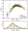 |
Fig. 9. Same as Fig. 4, but for the 2G2 stars in NGC 2808. |
| In the text | |
|
Fig. 10. Same as Fig. 2, but for the case of the eHB in NGC 2808 simulated as an individual group of stars. The dashed and the dot-dashed lines represent the canonical ZAHB of appropriate metallicity with Y = 0.28 and Y = 0.35, respectively. We also report the end of the canonical HB at the bottom. |
| In the text | |
|
Fig. 11. Same as Fig. 2, but for the case of the eHB in NGC 2808. Dashed and the dot-dashed lines represent the canonical ZAHB of appropriate metallicity with Y = 0.28 and Y = 0.35, respectively. |
| In the text | |
|
Fig. 12. Mass-loss increase (Δμ) vs helium enhancement (ΔY) of the stellar populations studied in this work. The two series of points refer to the stellar populations (SP) in NGC 6752 (red diamonds) and NGC 2808 (blue triangles). The two blue squares in the figure refer to the alternate description of the eHB in NGC 2808. In the figure, the data from Tailo et al. (2020) are also reported. |
| In the text | |
Current usage metrics show cumulative count of Article Views (full-text article views including HTML views, PDF and ePub downloads, according to the available data) and Abstracts Views on Vision4Press platform.
Data correspond to usage on the plateform after 2015. The current usage metrics is available 48-96 hours after online publication and is updated daily on week days.
Initial download of the metrics may take a while.