| Issue |
A&A
Volume 695, March 2025
|
|
|---|---|---|
| Article Number | A228 | |
| Number of page(s) | 24 | |
| Section | Catalogs and data | |
| DOI | https://doi.org/10.1051/0004-6361/202451340 | |
| Published online | 21 March 2025 | |
Flaires
A comprehensive catalog of dust echo-like infrared flares
1
Deutsches Elektronen Synchrotron DESY,
Platanenallee 6,
15738
Zeuthen, Germany
2
Institut für Physik, Humboldt-Universität zu Berlin,
12489
Berlin,
Germany
3
Fakultät für Physik & Astronomie, Ruhr-Universität Bochum,
44780
Bochum,
Germany
4
Leiden Observatory, Leiden University,
Postbus 9513,
2300
RA Leiden, The Netherlands
★ Corresponding author; jannis.necker@desy.de
Received:
2
July
2024
Accepted:
5
February
2025
Context. Observations of transient emission from extreme accretion events onto supermassive black holes can reveal conditions in the center of galaxies and the black hole itself. Most recently, it has been suggested these sources could be emitters of high-energy neutrinos. However, in most cases, it remains unclear whether this would be classified as the outcome of rejuvenated accretion or a tidal disruption event (TDE).
Aims. We expand on existing samples of infrared (IR) flares to compile the largest and most complete list available. A large sample size is necessary to provide high-enough statistics for distant and faint objects to estimate their rates. Our catalog is large enough to facilitate a preliminary study of the rate evolution with redshift for the first time.
Methods. We compiled a sample of 40 million galaxies. Using a custom, publicly available pipeline, we analyzed the WISE light curves for these 40 million objects using the Bayesian Blocks algorithm. We selected promising for dust echo candidates involved in transient accretion events and we inferred the luminosity, extension, and temperature of the hot dust by fitting a blackbody spectrum.
Results. We established a clean sample of 823 dust echo-like IR flares, dubbed the Flaires catalog. For 568 of them, we were able to estimate the dust properties. After removing 70 objects with possible contributions from synchrotron emission, the luminosity, extension, and temperature are consistent with dust echos. Estimating the dust extension from the light curve shape revealed that the duration of the incident flare is broadly compatible with the duration of TDEs. The resulting rate per galaxy is consistent with the latest measurements of IR-detected TDEs and appears to decline with increasing redshift.
Conclusions. Although systematic uncertainties may impact the calculation of the rate evolution, this catalog will enable further research of phenomena related to dust echos from TDEs and extreme accretion flares.
Key words: accretion, accretion disks / catalogs / galaxies: active / infrared: galaxies
© The Authors 2025
 Open Access article, published by EDP Sciences, under the terms of the Creative Commons Attribution License (https://creativecommons.org/licenses/by/4.0), which permits unrestricted use, distribution, and reproduction in any medium, provided the original work is properly cited.
This article is published in open access under the Subscribe to Open model. Subscribe to A&A to support open access publication.
1 Introduction
Accretion onto compact objects is the most efficient form of energy release of normal matter. The heaviest such objects are the supermassive black holes (SMBHs) that reside in the center of most galaxies (Magorrian et al. 1998). If matter is accreted onto the SMBH, it forms a luminous accretion disk, dissipating the gravitational energy throughout the electromagnetic spectrum (Lynden-Bell 1969; Rees 1984).
If a star passes too close to the SMBH, the tidal forces can rip it apart. The subsequent accretion of its debris can be seen as a luminous transient dubbed a tidal disruption event (TDE; Rees 1988). These can last several months to years, offering unique insights into the properties of previously inactive SMBHs (Kesden 2012; Mockler et al. 2019; Wen et al. 2022; Yao et al. 2023). They were originally discovered as X-ray transients with a soft, thermal spectrum (Komossa & Greiner 1999). However, the optical detection rate dramatically increased in recent years thanks to the advent of large time-domain survey instruments and TDEs are now frequently discovered by instruments such as Zwicky Transient Facility (ZTF; Bellm et al. 2018; van Velzen et al. 2021), All-Sky Automated Survey for Super-Novae (ASAS-SN; Kochanek et al. 2017, e.g. Holoien et al. 2014; Hinkle et al. 2021), and Panoramic Survey Telescope and Rapid Response System (Pan-STARRS; Chambers et al. 2016, e.g. Gezari et al. 2012; Chornock et al. 2013; Nicholl et al. 2019). Indeed, the optical regime became the dominating detection channel with tens of TDEs per year (Gezari 2021). In the future, this is expected to increase with the Legacy Survey of Space and Time (LSST) of the Vera Rubin Observatory, expanding to thousands of detections per year (van Velzen et al. 2011; Ivezic et al. 2019; Bricman & Gomboc 2020). However, the bulk of the emission is expected in the extreme-UV which is almost impossible to observe because of absorption by neutral hydrogen (Ulmer 1999; Lu et al. 2016). Consequently, TDEs have been detected in the UV (Gezari et al. 2006) with an expected increase to hundreds per year with the survey of ULTRASAT (Sagiv et al. 2014). However, the radiation energy released by TDEs can be absorbed by dust in the vicinity of the SMBH and re-emitted in the infrared (IR), with the peak in the emission seen between 3 to 10μm’ and a typical luminosity of 1042 to 1043 erg s−1 (Lu et al. 2016). This IR emission has been observed in follow-up studies of optically and UV-detected (UVO) TDEs (van Velzen et al. 2016; Jiang et al. 2016; Dou et al. 2016). The transient IR emission has also been used to identify TDE candidates (Mattila et al. 2018; Wang et al. 2018; Kool et al. 2020) and confirmed TDEs (Wang et al. 2022b). Searches for IR excesses in SDSS galaxies (Jiang et al. 2021a), (ultra)luminous IR galaxies (ULIRGs; Reynolds et al. 2022) and galaxies the nearby universe (Masterson et al. 2024) resulted in samples of tens to hundreds of flares. The amount of obscuring dust in these systems is much higher than in optically selected TDEs, which indicates that the optical TDE population is biased towards dust-free environments (Jiang et al. 2021b). The preference of optical TDEs for post-starburst host galaxies (Arcavi et al. 2014; French et al. 2016; Hammerstein et al. 2021) might be (at least partly) a consequence of this bias (Jiang et al. 2021b; Reynolds et al. 2022). These samples provides a rate measurement of O(10−5) galaxy−1 yr−1, which is consistent with recent measurements in the optical (Yao et al. 2023). While the first estimates of the rate were almost an order of magnitude lower (Donley et al. 2002) than the theoretically expected rate of around 10−4 galaxy−1 yr−1, there is discrepancy now of only a factor of 2–4. The rate in ULIRGS even seems to be up to two orders of magnitude higher (Tadhunter et al. 2017; Kool et al. 2020; Reynolds et al. 2022). This shows that the IR is an important detection channel of the same intrinsic events just with a larger amount of dust.
If the accretion onto the SMBH is continuous, we observe the object to be an active galactic nucleus (AGN), which is the most luminous steady source in the universe. Although the accretion is roughly constant, random fluctuation is inherent to AGN activity. These AGN flares can happen on a timescale from hours to years (Ulrich et al. 1997) and show brightness variations of the order of tens of percent (Berk et al. 2004). Apart from this, there is an increasing number of observations of AGN variability beyond the expected statistical fluctuations. The first class is a longterm decline or rise over several years together with a change in the spectral features (LaMassa et al. 2015; Gezari et al. 2017; Frederick et al. 2019; Yang et al. 2023) called changing-look AGNs. These are typically attributed to accretion rate changes (Husemann et al. 2016; Yang et al. 2023). In contrast to this, there is a class of major AGN flares that are characterized by a sudden increase in their UVO emission, which differentiates them from the changing-look phenomena and are attributed to a sudden rejuvenation of the accretion onto the SMBH (Graham et al. 2017; Trakhtenbrot et al. 2019). A possible trigger could be TDEs happening around the accreting SMBH (Chan et al. 2019; Ryu et al. 2024). However, discerning this emission from AGN native variability is difficult and very few candidates have been observed so far; for example, PS16dtm (Blanchard et al. 2017; Jiang et al. 2017; Petrushevska et al. 2023) and PS1-10adi (Jiang et al. 2019; Kankare et al. 2017).
Similarly to the dust echoes of TDEs, the dust around the SMBH can reprocess the electromagnetic emission and re-emit it in the IR (Barvainis 1987). Because the dust efficiently absorbs from the optical to X-ray wavelengths, the resulting dust echo is agnostic to the nature of the incident transient as long as the transient evolution timescale is smaller than the light-travel time to distances where the dust is stable. Therefore IR transient emission can be used to compile a sample of TDEs and extreme accretion events at the same time. Indeed, Jiang et al. (2021a) recently compiled a sample of Mid-infrared Outbursts in Nearby Galaxies (MIRONG), a similar ensemble of IR flares. Spectroscopic follow-up revealed the appearance of coronal lines and fading Balmer lines which suggests that most of these flares are dust echos of TDEs or extreme transient AGN accretion (Wang et al. 2022a).
Transient accretion events of SMBHs have been suggested as the sources of high-energy particles (Farrar & Gruzinov 2009). This is supported in particular by the detection by the Ice-Cube neutrino observatory of the flaring blazar TXS 0506+056 (IceCube Collaboration 2018) in coincidence with a high-energy neutrino alert (Aartsen et al. 2017). These alerts are sent out by IceCube in real time and followed up by many observatories (Necker et al. 2022; Stein et al. 2023). ZTF detected two transients connected to SMBH accretion that are coincident with two high-energy neutrino alerts: AT2019dsg (Stein et al. 2021), a spectroscopically classified TDE, and AT2019fdr (Reusch et al. 2022), a giant AGN flare (see Pitik et al. (2022) for an alternative interpretation). The unifying feature is a large dust echo. A systematically compiled sample of 63 similar flares based on optical ZTF detections revealed a third event: AT2019aalc, another giant AGN flare. The sample is correlated with IceCube’s high-energy neutrino alerts at 3.6σ (van Velzen et al. 2024), which suggests a significant contribution from these accretion events to the diffuse neutrino flux (IceCube Collaboration 2013). Two more flares from the MIRONG sample are coincident with high-energy neutrinos (Jiang et al. 2023), although one of them shares the neutrino association with AT2019fdr. While an additional search using the full neutrino data sample did not show any significant excess (Necker et al. 2023), the size of the accretion flare sample was small and restricted to flares with an optical counterpart detection by ZTF, which started observing in 2018. To harvest the full potential of the neutrino data, we require access to a sample that spans as much of the IceCube data-taking period since 2010, while also spanning as much of the sky as possible and does not rely on optical detections. Additionally, because neutrinos are not attenuated traveling through the universe, this sample should be as complete as possible.
In this paper, we present a catalog of IR flares detected by WISE that expands on existing samples by an order of magnitude. This catalog provides a unique opportunity to tackle both the rate evolution and the neutrino association because it covers the whole sky, extends to high redshifts, and goes back to the start of IceCube operations.
The paper is organized as follows. In Sect. 2, we describe the creation of the IR light curves and selection of dust echolike flares. In Sect. 3, we explore the most likely physical origins of these flares and evaluate the corresponding completeness of the resulting catalog in Sect. 4. We investigate the implications for the rate evolution in Sect. 5, followed by a discussion of our results in Sect. 6. Throughout this paper, we assume a flat ΛCDM cosmological model, with the parameters presented in Planck Collaboration VI (2020).
2 Data
WISE was launched at the end of 2009 and began surveying the sky in four bands at the beginning of 2010 until it was shut down after its nominal mission lifetime in 2011. The data products of this phase were combined under the name AllWISE. WISE was re-activated in 2013 with the primary science goal of discovering near-Earth objects (Mainzer et al. 2014), which is called the NEOWISE reactivation phase (NEOWISE-R). Since then it has continuously observed the sky in two bands at 3.4 μm and 4.6 μm (W1 and W2). In this work, we use AllWISE and NEOWISE-R data to identify dust echoes of possible extreme accretion events because the two filters cover the relevant wavelength range, the sampling rate of around two data points per year is sufficient, and the observations span around ten years. The latest available release includes data up to December 2021.
2.1 Parent galaxy sample
To figure out where in the sky to look for candidate IR flares, we need the positions of galaxies, referred to as our parent galaxy sample. To leverage the all-sky coverage offered by WISE, this sample should cover as much of the sky as possible. In addition, it should be as large as possible to make the final flare sample as comprehensive as possible. Although galaxy identification is most reliable with spectroscopic observations, no spectroscopic survey has the necessary sky coverage. To achieve the goals described above, it is necessary to move towards photometrically inferred classifications. The NEWS sample (Khramtsov et al. 2020) provided the best starting point at the start of our analysis with around 40 × 106 extragalactic objects identified by a machine learning algorithm based on WISE measurements from the AllWISE source catalog and PSF magnitude measurements from the Pan-STARRS Data Release 1 catalog. It is a large sample of galaxies with 98% purity and more than 98% completeness for objects with a g-band magnitude fainter than 19 mag, which applies to 99% of the sample. In addition, it already supplies the identifier in the AllWISE source catalog, which allows us to easily query the WISE database for the corresponding single-exposure measurements (see Sect. 2.2). However, to reject bright foreground stars and achieve high purity for faint sources, the NEWS sample excludes sources brighter than 14 mag in g and r-band.
To include nearby and therefore bright galaxies, we supplemented the NEWS catalog with the WISE-PS1-STRM sample (Beck et al. 2022). It also uses a neural network and WISE and Pan-STARRS photometry to infer object classifications and photometric redshifts. Although NEWS is highly complete below 19 mag, its completeness declines slightly towards this magnitude, so we selected objects with a g-band magnitude brighter than 20 mag (gFPSFMag ≤ 20) from WISE-PS1-STRM. To maintain a high level of purity, we selected probable galaxies (prob_Galaxy > 0.5), but only if the objects were within the bounds of the training set (extrapolation_Class = 0). We crossmatched the resulting 3.2 × 10⁶ objects to the NEWS sample based on the Pan-STARRS object identifier and found 9.6 × 10⁵ non-overlapping sources, which we appended to the parent sample.
To ensure the list of galaxies is as complete as possible in the local universe, we included the Local Volume Sample (LVS) from the NASA Extragalactic Database (NED-LVS; Cook et al. 2023). It contains around 1.8 × 10⁶ sources with a redshift up to z = 0.2. We include 6.7 × 10⁵ sources from NED-LVS that have no counterpart in our sample within a radius of 1″.
The resulting parent galaxy sample has 4.2 × 10⁷ sources. The majority is located in the northern 3/4 of the sky above δ ≳ −30° since both the NEWS and the WISE-PS1-STRM samples are based on Pan-STARRS data. All sources with δ ≲ −30° come from the NED-LVS.
For the around 1.8 × 10⁶ sources in NED-LVS, we take the redshift from that catalog and for another 3.2 × 10⁷ sources we take the photometric redshift estimate from WISE-PS1-STRM. In total, we have at least photometric redshift estimates for 3.4 × 10⁷ sources, around 80% of all sources in our parent sample.
2.2 Infrared light curves
WISE scans the sky continuously, taking 7.7 s exposures. Roughly every half year each point in the sky will be covered by the field-of-view for about 12 consecutive orbits for about a day. We used the PSF fit photometry measurements based on these single exposures from both the AllWISE and the NEOWISE-R periods to get information about the evolution of the IR luminosity over time. The notable difference is that the AllWISE photometry is measured at the position of the corresponding source in the AllWISE source catalog, while the NEOWISE-R data fits the position of the source and only references the associated AllWISE catalog source.
Because photometry measurements can be impacted by image artifacts, cosmic rays, blending of close sources, and stray light from the moon, it is important to select reliable data points. We required good image quality, no de-blending, no contamination by image artifacts, a separation to the Southern Atlantic Anomaly of more than 5°, and a position outside the moon mask.
The selection of data for each source depends on the origin of the individual source. For all sources in the NEWS sample, we got the AllWISE source catalog identifier based on the designation. We then downloaded all AllWISE multi-epoch photometry for this identifier and all associated NEOWISE-R single-exposure photometry. The sources from the WISE-PS1-STRM and the NED-LVS samples do not have an associated entry in the AllWISE database, so instead, we selected the data based on the position. The FWHM of the WISE PSF is around 6″ so we downloaded all the single exposure photometry (both AllWISE and NEOWISE-R) within that radius. This will include all data for extended or faint objects where the scatter in the best-fit position is large. However, it also poses the risk of including data points related to a neighboring object. In particular, the AllWISE data is prone to this mistake because it includes the single epoch measurements or upper limits also of faint objects that are only detected in the AllWISE source catalog. Since, in these cases, blending is certain to be an issue, the AllWISE photometry of an object might not pass the quality criteria mentioned above. Thus, it is not sufficient to simply select the closest AllWISE photometry. Instead, we addressed the issue by finding clusters of data points and associating the closest cluster with the corresponding source in the parent sample. We employed the clustering algorithm HDBSCAN (McInnes & Healy 2017) to find the clusters of data points. We selected all points that belong to the closest cluster if that cluster is within 1″. Additionally, we selected all data points within 1″, even if they belong to a different or no cluster at all. This allowed us to select the corresponding single epoch photometry where the positional scatter is large as well, while minimizing the risk of including unrelated data points.
We stacked the single epoch photometry for each visit to get a more robust measurement. To combine the counts measured at the instrument level, we calculated the photometric zero-point, ZPi,j, for each single exposure measurement, i, of visit, j, per band:
 (1)
(1)
where Vi,j is the apparent magnitude in the Vega system and Ci,j is the flux in instrument counts. For each visit, j, we calculated the median of the zero-point, ZPv,med,j, per band. The spectral flux densities for each exposure are then
 (2)
(2)
where Fv,0 is the zero magnitude flux density (Jarrett et al. 2011). Finally, the stacked flux density is the median of the spectral flux densities per visit and band. The uncertainty is the maximum of the standard deviation to the median and the Pythagorean sum of the individual measurement uncertainties. We noted some outliers with unreasonably high fluxes, probably caused by cosmic rays or spurious detections that escaped the WISE flagging or asteroids that are passing through the line of sight. We found that we can reject these if they deviate from the median by more than 20 times the 70th percentile.
For each light curve and band, we calculated the reduced chisquare,  , with respect to the median as a preliminary measure of the variability of the light curve. This allows us to identify quiescent light curves early in the analysis based on a low
  value. To establish a meaningful threshold, we ran the flare search algorithm as described in the next section for a sub-sample of 2 × 10⁶ light curves. It turned out that all light curves that show flaring have a value of
  in both bands. Around half of the sources do not pass this threshold and were not analyzed further (see Fig. 1).
2.3 Flare selection
To find any potential excess in the light curves we use the Bayesian Blocks algorithm (Scargle et al. 2013) as implemented in astropy (Astropy Collaboration 2022). It divides the light curve into intervals of constant flux. Fewer intervals are favored where the strength of the preference depends on a prior. We chose the empirically motivated prior for point measures for the number of change points,
 (3)
(3)
for a light curve with Nvisit visits (Scargle et al. 2013). We defined the quiescent state, namely, the baseline, as the lowest flux we measured across the light curve. This does not have to be one continuous interval but can be interrupted by excesses. To combine all baseline intervals into one measurement, we successively combined the blocks with the lowest spectral flux density with the baseline. The updated baseline is the mean of all data points in the baseline blocks and its uncertainty is the standard deviation. We stopped when there was no remaining block within 5σ of the baseline. All blocks not within the baseline are considered excess blocks. Adjacent excess blocks have been considered as one excess and its start and end are defined as the time of the first and last data point within the excess, respectively.
To efficiently analyze the O(106) light curves, we implemented the procedure in the ampel framework (Nordin et al. 2019), which provides high-throughput streaming of data and is capable of including user-contributed code in the form of so-called units. ampel pipelines are split into four stages called tiers. The Bayesian Blocks analysis is implemented in tier two as the unit T2BayesianBlocks (see Fig. 1).
The Bayesian blocks result lets us identify flaring behavior. In the next step, we aim to quantify the significance of the flare compared to the rest of the light curve to identify significant dust echo-like flares. We implemented the following cuts as another tier two unit T2DustEchoEval (see Fig. 1 for the corresponding numbers):
Flare region: an excess in at least one of the two WISE filters;
Flares coincident in both filters: a coincident excess in the other band;
ΔF/Frms > Frms/σF: dust echo strength, ΔF/Frms, higher than the significance of variability in the extraneous part of the light curve, Frms/σF (van Velzen et al. 2024), to make the distinction to stochastic AGN variability. Then, ΔF is the difference between baseline and peak flux, Frms the root-mean-square of the extraneous light curve and σF the standard deviation of the baseline. An example is shown in the first panel of Fig. 2;
Baseline before excess: at least one baseline data point before the excess;
Gap: a baseline data point not more than 500 d before the first detection of the excess. This criterion excludes flares that rise during the AllWISE period. An example is shown in the second panel of Fig. 2;
State transition: a segmentation of the excess into at least two blocks to reject state transitions or a difference in time between the first and last data point in the excess of no more than 3 yr;
NE > 1: more than one data point in the excess;
ΔF/σF > 5: a detection significance of the excess of at least 5σ with respect to the baseline;
Just started: if the excess consists of a single block at the end of the light curve we consider it too recent;
Around 7000 sources passed the above selection criteria. However, by visual inspection, the majority show an excess that is inconsistent with the sharp rise and subsequent decay expected for a dust echo of a single activating flare. An example is shown in the third panel of Fig. 2. To get a pure sample of dust echo-like flares, we calculated the e-folding rise and fade times as
 (4)
(4)
For the rise time, Δt is the time between the last baseline data point and the maximum of the light curve, F1 is the baseline spectral flux density, and F2 is the peak spectral flux density. For the fade time, Δt is the time from the maximum to the last data point in the excess, F1 is the peak spectral flux density, and F2 is the last measurement of the excess. We found that the following e-folding times result in a pure sample of 823 good dust echo candidates:
10. Fast rise and fade?: τrise < 1000 d and 400 d < τfade < 5000 d.
We dub this list of infrared flares the Flaires1 catalog. An example is shown in the right panel of Fig. 2. The cut on the rise time ensures that the lightcurve rises to its maximum quickly and does not peak late as in the example in Fig. 2. The maximum requirement on the fade time ensures that the brightness decreases over time. Requiring a minimum ensures that the peak epoch is not at the end of the excess, in which case τfade would be zero. The values are geared towards purity and were found by visual inspection of the selected flares and do not make a distinction based on the underlying physics. Consequently, some of the flares outside this parameter range are still good dust echo candidates, negatively impacting the completeness of this analysis (see Sect. 4).
2.4 Difference light curves
To analyze the flare properties, we sought to obtain light curves that only contain the contribution from the excess. To get this difference photometry, we subtracted the baseline, measured as described in the previous section from the data (see Sect. 2.2). The uncertainty is the Pythagorean sum of the baseline uncertainty and the uncertainty of the stacked data. The spectral flux, vFv, is then the difference spectral flux density, Fv, multiplied by the frequency, v, corresponding to the central wavelength of the WISE bandpass.
A caveat of using the single exposure photometry is that there is a bias for dim sources near or below the limiting magnitude of mW1 ≈ 16.0 and mW2 ≈ 14.9. The scatter due to instrument noise in single-exposure photometry still produces detections above these limits, biasing the baselines toward brighter values. This is known as the Eddington bias (Eddington 1913) and has been identified as an effect already for the Infrared Astronomical Satellite (Beichman et al. 1988) as well as for NEOWISE-R (Mainzer et al. 2014). Because the bias gets stronger the dimmer the sources, this will mainly impact the baseline measurements. As a crosscheck, we compared them with the magnitudes from the AllWISE source catalog for the selected dust echo-like flares. The AllWISE measurements are performed on stacked images, preventing the bias. On average, the AllWISE measurements are around 3% fainter in both bands. 90% vary within around ±25% in W1, and −75% to 20% in W2, respectively. The difference between the bands comes from the worse sensitivity of the W2 band. This shows that determining the baseline from long-term lightcurves are necessary, but can be improved by measurements based on stacked images.
To obtain the redshifts, we used the well-curated values from the NED-LVS, which are available for 135 sources. If they were not available, we used the photometric redshifts from WISE-PS1-STRM (411 sources). For 139 sources, we found redshifts in other catalogs (see Table 1). Where we found more than one match, we divided the matches into categories based on spectroscopic and photometric measurements and the match distance and took the mean of the best category. We calculated the luminosity per bandpass in the rest frame based on the luminosity distance
 (5)
(5)
where the subscript e indicates the rest frame quantities.
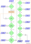 |
Fig. 1 Flowchart of the flare selection process. See Sect. 2.3 for a detailed explanation of the selection steps. |
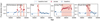 |
Fig. 2 Representative examples of the classification of the pipeline outlined in Fig. 1 for steps 3 (WISEA J063233+655809), 5 (WISEA J105052+000134), and 10 (WISEA J144620+371159) from left to right detailed in Sect. 2.3, which impact the completeness (see Sect. 4). The last panel shows one example of a dust echo-like flare (WISEA J083416-054249). The flux density in the W1 band is shown against time. The classification is annotated in the upper left corner. |
Number of matches in redshift catalogs.
3 Physical origin
3.1 Dust echo scenario
So far we established a sample of 823 objects showing an IR flare that is significant compared to the extraneous part of the light curve. Although we have already implicitly assumed that these IR excesses are dust echoes from nuclear flares in the selection process in Sect. 2.3, we analyze the physical properties corresponding to the dust echo scenario in more detail to check for consistency.
We assumed that the IR flares are due to reprocessed emission by dust, which is distributed in a thin, spherical shell around the central engine. We modeled the spectrum of the emission with a blackbody, although the dust emission is expected to follow a modified blackbody spectrum (Draine & Lee 1984). However, the resulting bolometric luminosity is almost unaffected while the temperature is only slightly lower (Jiang et al. 2021a). We fitted the rest frame luminosity in each band to the corresponding value predicted by the blackbody emission,
 (6)
(6)
to obtain a temperature, T, and an effective radius, Reff, for each visit. We numerically searched for the temperature that solves the ratio of Eq. (6) for the two bands. We used that to seed a maximum likelihood fit to obtain the best-fit values for T and Reff. To investigate how well the parameter space is constrained by the data and to derive uncertainties, we performed MCMC sampling and obtained posterior distributions using emcee (Foreman-Mackey et al. 2013). Because we fit the rest frame quantity  , we directly obtain the rest frame temperature. For each pair of fit parameters, we also calculated the bolometric luminosity as
 (7)
(7)
where σΒ is the Stefan-Boltzmann constant. To ensure a sufficient signal-to-noise ratio (S/N), we first required the luminosity ratio of the visit to be greater than its uncertainty. Secondly, we calculated the autocorrelation time, τ, of the MCMC ensemble (Sokal 1997). We stopped the chain after N iterations if N > 100τ, providing us with at least 100 independent samples per visit. If this condition is not reached after N = 10 000 iterations, the fit has not converged and we did not include the visit in the analysis. If the 69th percentile for the bolometric luminosity was larger than the best-fit value, we did not consider the sampling to give meaningful constraints. For 568 sources, we found at least two epochs with good constraints on the fit parameters. Figure 3 shows the resulting blackbody spectra for the flare with the highest fluence in our sample, located in the nearby galaxy NGC 7392. The derived parameters are shown in Fig. 4. They are in agreement with previous measurements that suggest it as one of the nearest TDE candidates (Panagiotou et al. 2023). The evolution of Lbol, T, and Reff for all 568 sources with at least two epochs with good constraints is shown in Fig. 5, as well as the bolometric flux,  . To calculate the total emitted energy, we integrated Lbol over the total duration of the flare in the source frame by linearly interpolating between measurements, so that
 (8)
(8)
where the sum runs over all N good fit epochs. The distribution is shown in Fig. 6. Although the peak of all flares was observed, the emission dimmed to pre-flare levels within the data-taking period before 2021 in only 243 cases. For the other 325 flares the energy estimate from Eq. (8) is only a lower bound. The flares that were observed entirely radiated on average around 45% of the total energy after the peak, so the energy of the flares that did not end before 2021 might be underestimated by a factor of two. To test whether the IR flares are dust echoes, we make sure that the derived parameters are consistent with this assumption.
Besides the hot dust, IR emission from relativistic electrons inside jets can contribute to the variability of the MIR light curves (Jiang et al. 2012; Liao et al. 2019). The same population of electrons typically also produces synchrotron emission in the radio band. To identify possible candidates for this emission, we matched our sample to the Million Quasars Catalog (Milliquas; Flesch 2023), the largest compilation of type-I quasars and AGNs. We found 86 matches within a search radius of 5″ where the maximum distance of any match we found is 1.4″. 70 objects are marked as core-dominated quasars, BL Lacs, or narrowline AGNs. We assumed that for most of these high-redshift objects, the IR emission comes from synchrotron emission, and we excluded these from further analysis. Consequently, the blackbody fits for some of those objects gave unreasonable high values for the bolometric energy, namely, Ebol ≳ 1053 erg s−1 (see Fig. 6).
To validate the dust radius obtained from the blackbody fits, we can compare it to the value estimated from the light curve shape. The dust echo light curve can be obtained from the light curve of the initial transient by convolving it with a tophat function. Its width, τ, is determined by the radius of the dust shell τ = 2 · R/c, where c is the speed of light (van Velzen et al. 2016). We can relate this to the bolometric light curve by dividing the integral by the peak:
 (9)
(9)
For a tophat function, this is a good approximation. Because we defined the bolometric energy as the integral in Eq. (8), the radius of the dusty region determined from the light curve is then
 (10)
(10)
If we want to compare this with the radius we get from the blackbody fits, we have to consider that at any time we only see a spatial slice of the dusty region due to the light travel time. We derived Reff assuming a blackbody with an area of  . However, because of the extension of the sphere, the surface area of the sphere that we see is ABB ≈ 2πRBB • cΔTopt where ΔTopt is the width of the activating flare. The relation between the effective and the actual radius is
 (11)
(11)
The comparison between RLC and the peak effective radius, Reff,peak, is shown in Fig. 7 with an indication for different values of ΔTopt using Eq. (11). For typical values for the duration of TDEs (Komossa 2015; Gezari 2021) the model is self-consistent, so we can take RLC as a reasonable estimate for RBB.
Moreover, the expected relation between the dust radius and the total bolometric energy is expected to be  (van Velzen et al. 2016). With Eq. (10), this implies that RLC ~ Lbol,peak. Assuming perfect blackbody emission, the relation between radius and temperature is RLC ~ T−2. Figure 8 shows these expected relations as the grey dotted line along with the measured values. There is a large scatter in all of the cases but the scaling of Ebol with the dust radius seems to fit the data reasonably well. Although there is no conclusion possible for the temperature and the peak bolometric luminosity, this further strengthens the dust echo model.
The temperature evolution in Fig. 5 is also consistent with cooling dust. Most of the flares start at a temperature of T < 2000 K which is broadly consistent with the sublimation temperature for the relevant dust grains (van Velzen et al. 2016), before cooling to lower temperatures of 600 to 800 K.
The total emitted energy falls in the range between a few times 1050 to 1053 erg with most of the events between 1051 to 1052 erg (see Fig. 6). We will discuss this in more detail in the next section, especially Sect. 3.2.3.
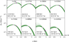 |
Fig. 3 Blackbody fits for NGC 7392 for all epochs of the flare where the MCMC sampling resulted in meaningful constraints on the fit parameters. The dashed green line shows the best fit and the transparent lines show the results from the MCMC sampling. The best fit and 68th percentile temperature and effective radius values are shown in the bottom left corner. The frequency, v, is given in the source frame. |
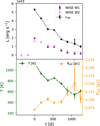 |
Fig. 4 Light curve and evolution of Reff and T for NGC 7392. The crosses mark the best-fit values of the visit where the MCMC sampling did not result in a meaningful constraint of Lbol . The results are consistent with Panagiotou et al. (2023). |
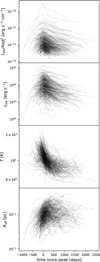 |
Fig. 5 Parameters from the blackbody fits for 449 sources where at least two epochs have a good fit. The time is given in the source frame. First panel: Bolometric flux based on the bolometric luminosity and the luminosity distance. Second panel: Bolometric luminosity (see Eq. (7)). Third and fourth panel: Temperature and effective radius (see Eq. (6)). |
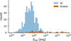 |
Fig. 6 Distribution of the total emitted energy, assuming hot dust (Eq. (8)). The quasars are identified by a match to Milliquas (see Sect. 3.1). |
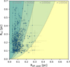 |
Fig. 7 Dust radius estimated from the IR light curve, RLC, against the radius at the peak, Reff,peak, obtained from the blackbody fits. The colored contours represent the actual blackbody radius for a finite width of the initial O/UV transient (see Eq. (11)). |
3.2 Possible nature of the initial transient
3.2.1 Contribution from AGNs
Variability in active galaxies is well known as well as delayed IR emission due to dust reprocessing (Ulrich et al. 1997). Although unusually bright IR flares compared to the extraneous part of the light curve were selected, hosts that exhibited AGN activity before the flare were not explicitly excluded. We can expect a certain percentage of the flares to be connected to the usual accretion onto the SMBH, so we tried to estimate their contribution to our sample.
We used the classification based on Baldwin -Phillips-Terlevich (BPT) diagrams (Baldwin et al. 1981) derived from SDSS spectroscopic observations (Brescia et al. 2015) to get robust classification of the host galaxies. We found 61 matches, of which 22 are star-forming galaxies, 19 composite objects, 11 AGNs, and 9 low-ionization nuclear emission line region (LINER) galaxies. Thus, at least one-third of the spectroscopically classified hosts do not show signs of AGN activity before the flare. However, this small subsample is not entirely representative as it is, on average, one magnitude brighter and the W1-W2-color is around 0.16mag bluer.
To look for possibly classified optical counterparts, we found 68 matches on the Transient Name Server2 (TNS). While 54 are unclassified, 6 objects are classified as AGN flares. However, at least five of them are unlikely regular statistical AGN variability. While a regular TDE origin was rejected for AT2017bgt, it was attributed to enhanced accretion onto the SMBH, a reignition of the active nucleus, and was used to define a new flare class (Trakhtenbrot et al. 2019). AT2018bcb shares similarities both with regular TDEs and the AT2017bgt-like flares (Neustadt et al. 2020). This is also true for the brightest flare in our sample in the nearby AGN NGC 1566 (Ochmann et al. 2024). The spectrum of AT2017fro was initially classified as a supernova type II (Brimacombe et al. 2017) and later found to be more consistent with an AGN (Arcavi et al. 2017). More detailed analysis revealed similarities with other nuclear transients of uncertain nature like CSS100217 (Drake et al. 2011) and AT2019fdr (Frederick et al. 2021; Reusch et al. 2022). It is found to be most compatible with a supernova type IIn in an AGN that triggered enhanced accretion activity but a TDE origin cannot conclusively be ruled out (Holoien et al. 2022). AT2019avd is an extensively studied nuclear flare in a previously inactive galaxy that shows X-ray properties consistent with a TDE scenario although the optical and UV emission is less TDE-like (Malyali et al. 2021). It has also been suggested as a turn-on AGN event (Frederick et al. 2021) similar to AT2017fro, as a partial TDE (Chen et al. 2022) or a particular type of jetted TDE (Wang et al. 2023). AT2018dyk was classified as a TDE (Arcavi et al. 2018; Huang et al. 2023) but also interpreted as an AGN turn-on due to the spectroscopic evolution from a LINER into a Seyfert state (Frederick et al. 2019). AT2022sxl was classified as an AGN flare (Reguitti 2022), but is unrelated because it happened roughly six years after the IR peak. In summary, all the reported optical AGN flares in our sample are not due to standard statistical AGN variability but, rather, to isolated events associated with the enhanced accretion onto the SMBH; whereas the exact nature of the trigger of this enhancement is less clear.
To investigate the total contribution of flares happening in AGN hosts, we classified the galaxies based on their red IR color. We do not use the measured baseline magnitudes because of the biases affecting dim sources (see Sect. 2.3). The redder band W2 is less sensitive and the bias more prominent, reddening the measured color, in particular for blue sources. So using the measured baseline leads to an overestimation of the percentage of AGN hosts. Instead, the magnitudes derived from stacked WISE images from the parent sample catalogs were used.
Employing the common selection cut on the magnitude difference between the W1 and W2 bands, mW1 − mW2 > 0.8 (Stern et al. 2012), the percentage of hosts with signs of AGN activity in our flare sample is 14%. While it does increase from 6% in the parent galaxy sample, it still shows that most of the hosts do not have strong contributions from a pre-existing AGN. Almost no AGNs (≲2%) have a color of mW1 − mW2 < 0.5 (Stern et al. 2012). Around 54% of the flare hosts lie in this AGN-free color space and 82% of the total parent galaxy sample.
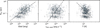 |
Fig. 8 Correlation of the total emitted bolometric energy Ebol, the peak bolometric luminosity Lbol,peak and the dust radius infered from the light curve RLC. The dashed lines represent the theoretically expected relations. |
3.2.2 Contribution by supernovae
Infrared emission from hot dust after supernova explosion has been studied in the past and some supernovae remain detectable in the IR even decades after explosion (Tinyanont et al. 2016). It is therefore worth looking for supernovae also in our sample. We found six matches with transients classified as supernovae on TNS. We suggest, however, that at least two of them could instead be flares connected to the accretion onto the SMBH.
SN 2018gn was first classified as a type II supernova (Falco et al. 2018) but recently interpreted as a dusty TDE based on the large dust echo and the emergence of coronal lines (Thévenot et al. 2021a; Wang et al. 2024) and is part of the sample of IR detected TDEs by the WISE Transient Pipeline (Masterson et al. 2024). SN 2020edi was classified as a superluminous supernova of type II in the center of an AGN (Tucker 2021). Its very luminous dust echo was previously reported (Thévenot et al. 2021b) and, correspondingly, our inferred bolometric energy of almost 1052 erg matches that of the other nuclear transients. Spectroscopic follow-up observations could determine the emergence of coronal lines, similarly to SN 2018gn.
We did not find any evidence that the remaining four supernovae are instead connected to SMBH accretion. Three show spectral features interpreted as signs of interaction with the circumstellar medium and are classified as type IIn: SN 2020iq (Dahiwale & Fremling 2020), SN 2018ctj (Fremling & Sharma 2018) and 2018hfm (Zhang et al. 2022). We note that SN 2020iq has a very high inferred bolometric energy of around 2 × 1051 erg. The distance to the closest source detected with Pan-STARRS is around 0.4″ which puts it at an angular diameter distance of roughly 700 pc from the host center, supporting the supernova interpretation. Comparing to a list of IR detections of supernovae (Thévenot et al. 2021a,b), its absolute magnitude of MW1 ≈ −24 magVega and MW2 ≈ −25 magVega is brighter than other type IIn supernovae by about two magnitudes, and more similar to superluminous supernovae (SN 2020edi and SN2020usa; Pitik et al. 2023) and transients interpreted as TDEs after their initial supernovae classification (SN 2016ezh/PS16dtm (Blanchard et al. 2017; Jiang et al. 2017; Petrushevska et al. 2023) and SN 2018 gn). SN 2018ktv was classified as a type IIL (Fremling et al. 2019).
To also check for supernova detections before the introduction of the TNS, we crossmatched with two lists of supernovae. The first3 is a compilation of supernova reports from different channels (TNS, ATELs, IAUCs, CBATs, and the TOCP web page; Gal-Yam et al. 2013). The crossmatch was performed for all archived objects between 2009 and 2021. The second one lists the supernovae detected by ASAS-SN4. Besides ASASSN-18xl/AT2018hfm, ASASSN-18ap/AT2018gn, and ASASSN-17jz/AT2017fro which are described above there were no additional matches.
To confirm that the IR flares are indeed happening in the center of the host galaxies, we calculated the offset of the position of the data related to the flare to the position of the baseline data. We found all three supernovae above with a separation of more than 0.5″. We find 36 more sources with an angular separation at least as high but for only three of them, the offset seems real. The rest likely suffer from inaccurate photometry or confusion of the host galaxies (see Appendix C). The high angular separation suggests that these objects are supernovae, bringing the total number up to six. This implies a contamination in our sample by only around 1%. Therefore, we find that the contribution of supernovae in our sample is subdominant, consistent with the conclusion for the MIRONG sample (Jiang et al. 2021a).
3.2.3 Transient accretion events
The previous two sections concluded that the sample is neither dominated by supernovae, nor by regular AGN activity. However, as mentioned in Sect. 3.2.2, the flares do happen in the center of their host galaxies. Because all derived physical parameters are consistent with the dust echo of an initial flare happening in a dust shell with R ≈ O(10−1 pc), this makes them likely dust echos of extreme accretion events onto the SMBH. The inferred bolometric energy is 1051 to 1052 erg which is roughly an order of magnitude higher than the estimate for most of the (candidate) supernovae but consistent with the energy output of a TDE, assuming a covering factor of fc ≳ 0.1, the disruption of a solar mass star, subsequent accretion of half its mass and a dissipation efficiency of ϵ ~ 0.1.
Indeed, roughly half of the 39 brightest flares are already classified as either TDE candidates or peculiar AGN flaring activity (see Table A.1). As mentioned in Sect. 3.2.1, the brightest flare in our sample in the nearby AGN NGC 1566 shares similarities with both TDEs and peculiar AGN flares (Ochmann et al. 2024) similar to AT2017gbt (Trakhtenbrot et al. 2019) which is the fourth brightest flare in our sample. Both the second and third brightest flares are promising candidates for IR-detected TDEs (Panagiotou et al. 2023; Masterson et al. 2024) as well as seven other flares. An additional five of the 39 brightest are part of the MIRONG sample (Jiang et al. 2021a). Also, the 14th brightest flare AT2019avd is a potential TDE (Malyali et al. 2021).
Absolute and relative numbers of the results of our pipeline for three reference samples
4 Completeness
To make any firm statement about a population of astrophysical sources, it is vital to understand the fraction of sources that are missing from the underlying catalog. In principle, there are three distinct reasons for the loss: the incompleteness of survey area, depth, or limited detection efficiency in the survey volume. In the case of this study, the first point is linked to the choice of the parent galaxy sample, while the selection efficiency results from the Bayesian blocks analysis and subsequent cuts. The depth is influenced by both as the parent galaxy sample will be less complete at higher redshifts and also the selection efficiency is worse for fainter signals. In the following, we focus on detection efficiency before discussing the parent galaxy sample and depth.
The detection efficiency is a convolution of the detection efficiency of WISE and the selection efficiency of our pipeline. Because each step would require its own set of dedicated simulations, which is beyond the scope of this paper, we instead estimate the efficiency of our selection by comparing our sample to results from the literature. The results per object are listed in Table B.1
Masterson et al. (2024) identified 18 candidates for IR-selected TDEs using the WISE Transient Pipeline (WTP). These candidates were selected based on their high peak luminosity, fast rise, and monotonic decline, with no underlying AGN host or signs of prior variability. Table 2 shows a summary of the results of our pipeline for this sample. We classified exactly half of these flares as dust echo-like, while four candidates were classified as long flares. Another four got rejected because the flare is not sufficiently strong compared to the variability of the rest of the light curve. One flare did not have a baseline detection before the excess. Because the selection is based on a crossmatch against a galaxy catalog that extends up to about 200 Mpc (Cook et al. 2019), the WTP TDE sample does not pick up candidates beyond a redshift of z ≲ 0.045. Among the 40 brightest flares in our sample, only 13 are below this redshift. Six of those are not included in the WTP TDE sample (see Table A.1).
The MIRONG sample (Jiang et al. 2021a) followed a similar approach of collecting WISE photometry for a parent galaxy sample. The selection of candidate variable galaxies is based on the difference between the maximum and minimum brightness. Distinct outbursts are selected based on the brightness increase from the baseline to the peak. The result is a sample of 137 flares. Only 33 (24%) of those were selected as dust echo-like by our pipeline (see Table 2) while 40 are long flares and 35 show signs of extraneous activity (55%). Three of the galaxies are missing from our parent galaxy sample, all of which are at a high redshift between 0.2 and 0.3 compared to the other galaxies. The remaining 26 flares (19%) got rejected based on their data quality because we either found the excess to be attributed to an outlier or the peak takes place during a longer gap in the data, or because there was no baseline detection before the flare. In two cases, the rejection is related to the initial selection of photometry data points described in Sect. 2.2: the coordinates of SDSSJ010320+140149 are too far away from the WISE measurements, which are centered on its nucleus, so our data selection rejects the photometry as unrelated. The data points that constitute the flare in SDSSJ153151+372445 are significantly offset from the nucleus and also rejected by our photometry selection. The resulting light curve does not pass the initial variability cut on  . Using the parent galaxies of the MIRONG sample (SDSS spectroscopic galaxies below a redshift of z < 0.35 ), we verified that only 20 of our objects were not included in that sample. Among them, only the flare in WISE J170944.87+445042.2 peaks before the end of 2018, the period included in MIRONG. It is faint (
 ), but clearly detectable over at least three visits. The difference between the dimmest and brightest data point is only around 0.4 mag in W1, which is below the required 0.5 mag increase required by the MIRONG selection. Concerning the sky coverage, we can conclude that our sample represents a clean expansion of MIRONG.
Both the previously mentioned samples and the analysis in this work rely on cataloged host galaxies. Because galaxies have to be bright enough to enable observations that are sufficient for such a classification, both intrinsically dim and far away hosts are likely missing from such catalogs. A possibility to decouple the IR flare search from the host parameters is to rely on a different tracer of possible locations of the flare. van Velzen et al. (2024) used nuclear flares detected in the optical by ZTF and searched for IR flares at the same position using WISE data. The selection of the optical flare only relies on the detection of the host to determine the angular offset but not a classification. The result is a sample of 63 optical transients with large dust echos that are likely TDEs or high-amplitude AGN flares. To highlight this unification, they are dubbed accretion flares (ZTF AFs from now on). 22 of these flares were classified by our pipeline as dust echo-like (35%, see Table 2). Most of the rejected events (around 27%) did not pass the cut on extraneous activity while 14% were classified as long flares. For AT2019pev we only found one data point in one band in the single exposure photometry because most of the data points are excluded due to de-blending (see Sect. 2). For AT2018jut and AT2019dll we did not find an excess in both bands and for AT2020aezy no excess at all. This is because the significance of the excess is not high enough to be recognized by the Bayesian blocks but high enough to pass the significance threshold when using the expected flare start time based on the optical flare. This highlights the advantage due to prior knowledge about the IR excess time. For AT2021aeuh and AT2019msq the flux in the AllWISE single epoch photometry is systematically lower than in the NEOWISE-R photometry which leads to a false identification of the whole NEOWISER period as a flare. The objects are then rejected because the peak of that supposed flare would fall in the gap between 2011 and 2014. The hosts of another 14% are not included in our parent galaxy sample. Those galaxies are on average one magnitude dimmer in the WISE bands and also redder, indicating that they are further away although redshift measurements are necessary for confirmation.
The results for these samples combined suggest completeness of the selection procedure of roughly 25-50%, where the main losses are attributed to our definition of long flares and extraneous activity. However, we remind the reader that these cuts are necessary to exclude AGN variability as the source of the IR flares as described in Sect. 3.2.1.
As previously mentioned, the completeness in absolute numbers per volume also depends on the completeness of the parent sample since it provides the positional information. Assessing its completeness is complicated, especially because it is not derived from a homogenous survey sample but from three different catalogs (see Sect. 2.1). If these catalogs were homogenous over the whole sky, one could in principle obtain the completeness by comparing to a small and deep observation and extrapolate that to the rest of the sky. However, because two of the three parent sub-samples make use of Pan-STARRS data, the sky below a declination of around −30° is sampled significantly worse. Another possibility is to compare the cumulative luminosity included in our sample to a measured luminosity function. However, there exists no such measurement based on the WISE filters5. We do therefore not attempt to calculate the completeness ourselves. But because we included all NED-VLS sources, a lower estimate of our sample’s completeness is given by the completeness of the NED-LVS, which is highly complete in the very nearby universe up to 30 Mpc, around 70% complete to 200 Mpc and drops to about 1% at 1 Gpc (Cook et al. 2023). Because we include many more faint sources, we can expect that our parent sample improves on this, especially at high distances.
5 Implications for the rate and its evolution
We establish in Sect. 3.2 that the flares in our sample are likely TDEs or at least enhanced accretion states. It is worth exploring the resulting rate of the events and comparing them with results from other samples. If the rate is in line with other TDE rate measurements it would indicate a high contribution of TDEs in our sample. Furthermore, because of the large size of our sample, we can investigate the evolution of this rate with redshift. Doing this per volume and time would require a better understanding of the completeness of our parent sample (see Sect. 4) so instead we focus on the rate of events per galaxy.
Because TDEs should only happen around black holes with masses lower than the Hills mass, mbh ≈ 108 M⊙ (Hills 1975), it is useful to look at the rate as a function of the black hole mass. Because we cannot directly access it, we used the host absolute magnitude in W1, MW1, as a proxy. There exist empirical relations between the host stellar mass and the black hole mass with different parameters for elliptical galaxies and AGNs (Reines & Volonteri 2015). The host absolute magnitude in W1, MW1, can in turn be used as a proxy for the stellar mass (Kettlety et al. 2018). Combining the two relations we use MW1 as a proxy for mBH. For elliptical galaxies, the Hills mass corresponds to MW1 ≈ −23magVega, whereas for AGNs, that is MW1 ≈ −26magVega. The histograms in Fig. 10 show the absolute number of flares and parent galaxies as a function of redshift and MW1. We find that the flares happen in galaxies with MW1 from −20.5 to −27.5magVega with the majority between −23 to −25 magVega. This would imply that most of the flares cannot be due to TDEs because the SMBH is above the Hills mass using the relation for elliptical galaxies. In that case, they would be AGN flares and we would have to use the corresponding relation, resulting in a SMBH mass below the Hills mass. Because of this kind of flip-flopping, we cannot conclude on the absolute magnitudes of the hosts alone. Instead, we looked at the evolution of the rate in each magnitude bin.
The rate for magnitude bin, i, and redshift bin, j, is
 (12)
(12)
where T is the sampling time, Nflare,i,j is the number of flares, and Ngal,i,j the number of parent galaxies in the respective bin. Also,  is the median redshift value of bin j and accounts for the time dilation of the observed rate with the cosmic expansion. The uncertainty is the 95th-percentile Poisson confidence interval based on Nflare,i,j.
The last NEWOWISE-R data release that was included in the analysis includes data up to December 2021. Because we started with data from AllWISE, the naive estimate for the sampling time would be around 11 yr between January 2010 and December 2021. However, because the WISE satellite was inactive between February 2011 and December 2013 there is around 1.5 yr gap in the data. Also, we required a baseline detection before the flare and at least two detections of the flare (see steps 4 and 9 in Sect. 2.3). Because there is on average a visit every six months, each of these two requirements deducts about 0.5 yr. The naive estimate of the sampling time would then be about 8 yr. In reality, the effective sampling time is shorter, due to edge effects near the start, end, and break of the dataset. To include this effect, we used the average rate of flares per time, Rref, within a reference window and compared it to the overall observed rate, Robs. Assuming that the true astrophysical rate of flares is approximately constant over time, the effective sampling time is then just the total time from the start of WISE observations until the last included data point, scaled according to the ratio of observed to expected rate. Because the rates are just the number of observed flares, N, over the corresponding time window, this can be simplified to
 (13)
(13)
Figure 9 shows the distribution of flare peak dates. We observe Nref = 507 flares in our reference region from around May 2016 to June 2020 and Nobs = 753 flares in total, giving an effective sampling time of Teff = (6.1 ± 0.3) yr. We adopt this as our sampling time T.
The rates are shown in Fig. 10. We measured the highest rate at MW1 = [−26, −24]magVega and z < 0.05 to be ![${{\cal R}_{[ - 26, - 24], < 0.05}} \approx 3.7_{ - 1.7}^{ + 2.6} \times {10^{ - 5}}\,{\rm{galax}}{{\rm{y}}^{ - 1}}\,{\rm{y}}{{\rm{r}}^{ - 1}}$](/articles/aa/full_html/2025/03/aa51340-24/aa51340-24-eq25.png) galaxy−1 yr−1). The rate shows a rapid decrease towards brighter galaxies and a shallower towards the fainter end. To obtain the evolution of the rate with redshift, we need to consider the loss of sensitivity. Figure 11 shows the distribution of the bolometric luminosity at peak as a function of redshift relative to the number of galaxies in the respective redshift bin. The evolution of the luminosity distribution shows the expected loss of sensitivity at low luminosities because dimmer flares are harder to detect at higher redshifts. Because we still detected flares with Lbol,lim ≈ 6 × 1043 erg in all redshift bins, we made the simplifying assumption, that our search is efficient in detecting flares with Lbol,lim up to the highest considered redshift bin.
galaxy−1 yr−1). The rate shows a rapid decrease towards brighter galaxies and a shallower towards the fainter end. To obtain the evolution of the rate with redshift, we need to consider the loss of sensitivity. Figure 11 shows the distribution of the bolometric luminosity at peak as a function of redshift relative to the number of galaxies in the respective redshift bin. The evolution of the luminosity distribution shows the expected loss of sensitivity at low luminosities because dimmer flares are harder to detect at higher redshifts. Because we still detected flares with Lbol,lim ≈ 6 × 1043 erg in all redshift bins, we made the simplifying assumption, that our search is efficient in detecting flares with Lbol,lim up to the highest considered redshift bin.
We then calculated the relative rate in redshift bin, j, as
 (14)
(14)
where Nlim,i,j is the number of flares with Lbol > Lbol,lim in the respective magnitude and redshift bin. Because we are only interested in the relative evolution and not the absolute value, we only summed over the three bins M, that contain at least one flare with Lbol > Lbol,lim in any redshift bin. The relative rate is shown in Fig. 12 along with the relative rate for the two magnitude bins, where we found a flare in the first and at least one other redshift bin. The results for the two lower magnitude bins (Mw1 = [−26, −24] magVega and Mw1 = [−24, −22]magVega) suggest a strictly negative evolution with a decreasing rate with higher redshifts. The evolution of the rate of TDEs based purely on the density of SMBHs predicts a shallower decline (Sun et al. 2015; Kochanek 2016). If TDEs do prefer post-starburst host galaxies (Arcavi et al. 2014; French et al. 2016; Hammerstein et al. 2021) which are more abundant at higher redshifts (Wild et al. 2016), the expected rate could even increase although the exact evolution is unclear. As mentioned above, even for AGNs, the Hills mass corresponds to a host absolute magnitude of MW1 ≈ −26 magVega, which would make the flares in the highest host magnitude bin, MW1 = [−26, −28] magVega, more likely to exhibit AGN activity than that of a TDE. Thus, it would be interesting to see if the evolution of that bin is similar to the lower magnitude ones. Unfortunately, no flares above Lbol,lim are observed in the first two redshift bins.
In summary, the rate seems to agree with previous results from IR-detected TDEs and the evolution, measured for the first time, is consistent with being strictly negative. We conclude that this indicates that the majority of flares in our sample are likely TDEs.
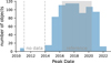 |
Fig. 9 Distribution of peak dates over time. The reference time window from around May 2016 to June 2020 is indicated as the grey-shaded region. The break of WISE data taking is indicated with grey dashed lines. |
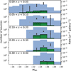 |
Fig. 10 Rate as a function of the absolute magnitude in W1 and redshift. The light blue histogram shows the total number of galaxies in the parent galaxy sample and the green one is the host of our flare sample. The black hatched bars represent flares with Lbol,peak < 6 × 1043 erg. The grey data points and black errors show the rate as calculated with Eq. (12). The grey triangles are the 90% upper limit on the rate where no flare was observed. The errors are statistical only. |
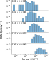 |
Fig. 11 Distribution of the maximum bolometric luminosity as a function of redshift. |
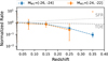 |
Fig. 12 Evolution of the rate with redshift for the two MW1 bins where there are flares in the first and at least one other redshift bin, normalized to the first redshift bin. Open symbols represent upper limits. The redshift evolution of the star formation rate (SFR) Madau & Dickinson (2014) and for TDEs Sun et al. (2015) is shown for comparison. |
6 Discussion and conclusion
In this work, we present a pipeline capable of building IR light curves based on WISE data for millions of objects and efficiently filtering them to get dust echo flare candidates. We have used the pipeline, together with a parent galaxy sample that covers more than three-quarters of the sky, to obtain the largest sample of IR flares compiled to date. We (at least) doubled the sky area included in the analysis, as compared to a previous study (MIRONG sample; Jiang et al. 2021a) by not relying on SDsS observed parent galaxies. We greatly expanded the observed volume compared to the latest sample of IR-selected TDE candidates by Masterson et al. (2024). The result is a sample of around 800 flares that last for thousands of days with a peak luminosity of 1043 to 1045 erg s−1 and a peak dust temperature of 1000 to 2000 K. We deduced that the incident transient has a width of 100 to 1000 d. This is consistent with dust echoes and the inferred parameters are broadly consistent with TDEs, although we cannot exclude extreme accretion events in AGNs. We determined the rate per galaxy, which is consistent with measurements of IR-detected TDEs in the local universe (Masterson et al. 2024). The sample is deep enough to allow a preliminary study of the evolution of the rate with redshift, which is consistent with a negative evolution.
There are two caveats with respect to the compilation of our sample. The biggest one remains the contribution of AGN activity. Because our selection takes into account the pre-flare variability, regular AGN variability is unlikely to be a significant contribution (see Sect. 3.2.1). However, although we selected dust echoes by obscured TDEs or extreme accretion events, we cannot distinguish between these two scenarios based on the IR data. One indication would be the mass of the black hole, which is most accessible through spectroscopy. Observations of the host galaxies could improve our crude estimate in Sect. 5 and determine if indeed there is a population of flares in hosts with mBH > 108MΘ. For those, a TDE origin would be unlikely.
Another caveat is the Eddington bias affecting measurements near the detection limit of the single-exposure photometry (see Sects. 2.3 and 3.2.1). Although we verified that the effect on the baseline measurements does not impact our result, the exact values for the luminosities of dim sources should still be taken with care. We cannot exclude the possibility that the flare luminosities at higher redshifts are systematically too bright. In that case, the detection threshold would be smaller and, as a result, we would end up including more flares at lower redshifts in the evolution calculation, making the rate fall even more steeply towards higher redshifts. To overcome this bias, photometry based on stacked images is necessary to make sure that epochs are also included where the source brightness is below the single-epoch limit.
Finally, we note that the results for the rate and its evolution presented in this analysis do not constitute a conclusive measurement; rather, we aim to evaluate their consistency with a TDE origin. The selection efficiency especially suffers from the strict cuts necessary to distinguish regular AGN variability (see step 3 in Sect. 2.3). These cuts are sensitive to the uncertainty of the baseline measurement, σF, which is small for bright flares and the resulting selection threshold is especially constraining. Consequently, the selection efficiency is likely worse for bright, nearby flares. Defining selection cuts without relying on the uncertainty of the baseline measurement could mitigate this, but a detailed study is necessary to tune these new cuts. We investigated the effects of relaxing the cut on extraneous variability by requiring the dust echo strength to be greater than the significance of extraneous variability or 5, effectively capping the significance of extraneous variability. We found 329 additional flares, many of which seem to be due to non-thermal emission by quasars, but are not listed in Milliquas. The brightest dust echo-like flare that passes due to this relaxed cut is AT2019aalc, a nuclear transient claimed to be coincident with a high-energy neutrino (van Velzen et al. 2024). We also recovered AT2017gbl, a obscured TDE candidate (Kool et al. 2020). The resulting rate and evolution did not change significantly. Thus, while the sample would be more complete and the resulting rate and evolution more robust, our conclusion would not significantly change. On the other hand, flares at higher redshift will appear stretched due to time dilation and might be harder to select against brightness changes on longer timescales. Correctly taking this bias into account can lead to a shallower decline towards higher redshifts. Furthermore, the selection effects induced by our pipeline presented in Sect. 2.3 are only characterized relative to two reference samples. To evaluate the completeness of the parent galaxy sample, especially as a function of redshift, either an independent measurement of the galaxy luminosity functions in the WISE bands would be necessary; alternatively, photometric observations in bands with determined luminosity functions could be useful. Additionally, as previously mentioned, an absolute calibration would entail detailed simulations, which is beyond the scope of this analysis.
In summary, we have demonstrated that it is possible to compile a large and deep sample of IR flares using existing instruments. We show that this sample is deep enough to qualitatively study the rate evolution of TDEs with redshift. However, we note that more reliable photometry is necessary to obtain a quantitative result.
Data availability
The full version of the catalog (Table A.1) is available in electronic form at the CDS via anonymous ftp to cdsarc.cds.unistra.fr (130.79.128.5) or via https://cdsarc.cds.unistra.fr/viz-bin/cat/J/A+A/695/A228. The columns are described in Appendix A. The efficient download, stacking, and calculation of  as a preliminary variability metric as described in Sect. 2.2 is implemented in the publicly available python package timewise available at https://timewise.readthedocs.io/en/latest/ (Necker & Mechbal 2024). The flare selection pipeline described in Sect. 2.3 is publicly available as the timewise Subtraction Pipeline python package, timewise-sup, available at https://jannisnecker.pages.desy.de/timewise_sup/docs (Necker 2024). The code to reproduce the analysis can be found at https://gitlab.desy.de/jannisnecker/air_flares
Acknowledgements
JN, TP and PMV acknowledge support by the Helmholtz Weizmann Research School on Multimessenger Astronomy, funded through the Initiative and Networking Fund of the Helmholtz Association, DESY, the Weizmann Institute, the Humboldt University of Berlin, and the University of Potsdam. AF and PMV acknowledge support from the German Science Foundation DFG, via the Collaborative Research Center SFB1491: Cosmic Interacting Matters - from Source to Signal. This research was supported by a Grant from the German-Israeli Foundation for Scientific Research and Development (GIF, Grant number I-1507-303.7/2019). This publication makes use of data products from the Near-Earth Object Wide-field Infrared Survey Explorer (NEOWISE), which is a joint project of the Jet Propulsion Laboratory/California Institute of Technology and the University of Arizona. NEOWISE is funded by the National Aeronautics and Space Administration. Software: astropy (Astropy Collaboration 2022), emcee (Foreman-Mackey et al. 2013), scipy (Virtanen et al. 2020), scikit-learn (Pedregosa et al. 2011), pandas (McKinney 2010), numpy (Harris et al. 2020), matplotlib (Hunter 2007).
Appendix A Catalogue
Table A.1 lists the first 39 brightest flares in our sample. Below we describe each column of the full catalog which is available online.
Glossary
RAdeg [°]: Right Ascension in degrees
DEdeg [°]: Declination in degrees
HostWlmag: Host W1 magnitude (Vega)
HostW2mag: Host W2 magnitude (Vega)
NEWS: Index in the NEWS sample
AllWISE: AllWISE Designation of the Host
PS1: Object identifier of the host in Pan-STARRS
WISEAllSkycntr: Counter of the host in WISE AllSky
WISEAllSkyDesignation: Designation of the host in WISE AllSky
NEDLVSIndex: Index of the host in NED-LVS
NEDLVSName: Name of the host in NED-LVS
ParentSample: Index in the Flaires parent galaxy sample
e_z: Uncertainty of the redshift
zsource: The source where the redshift value was taken from
SDSSdist [″]: Distance to the associated SDSS object
SDSSclass: BPT class of the associated SDSS object
TNSdist [″]: Distance to the associated TNS object
TNSobjtype: Type of the associated TNS object
TNSname: Name of the associated TNS object
TNSdate: Discovery date [MJD] of the associated TNS object
milliquasdist [″]: Distance to associated Milliquas object
milliquastype: Broad Type of the associated Milliquas object
MirongName: Name of the host in the MIRONG sample
WTPName: Name of the object in the WISE Transient Pipeline TDE sample
RefTime [MJD]: Observer frame mean peak time in MJD
x2W1: χ2 value w.r.t. the median spectral flux density in W1
npointsW1: Number of Detections in W1
FmedW1 [mJy]: Median spectral flux density in W1
x2W2: χ2 value w.r.t. the median spectral flux density in W2
npointsW2: Number of Detections in W2
FmedW2 [mJy]: Median spectral flux density in W2
FbslW1 [mJy]: Measured baseline spectral flux density in W1
e_FbslW1 [mJy]: 1σ uncertainty on FbslW1
FbslW2 [mJy]: Measured baseline spectral flux density in W2
e_FbslW2 [mJy]: 1σ uncertainty on FbslW2
startW1 [MJD]: MJD of the first epoch of the determined excess in W1
endW1 [MJD]: MJD of the last epoch of the determined excess in W1
endedW1: True if the last epoch of the excess in W1 is the last available data point
startW2 [MJD]: MJD of the first epoch of the determined excess in W2
endW2 [MJD]: MJD of the last epoch of the determined excess in W2
endedW2: True if the last epoch of the excess in W2 is the last available data point
strengthW1: Dust echo strength in W1
strengthW2: Dust echo strength in W2
varW1: Significance of the extraneous variability in W1
varW2: Significance of the extraneous variability in W2
MaxFluxW1 [mW m−2]: Maximum flux density in W1
e_MaxFluxW1 [mW m−2]: 1σ uncertainty on MaxFluxW1
MaxFluxW2 [mWm−2]: Maximum flux density in W2
e_MaxFluxW2 [mW m−2]: 1σ uncertainty on MaxFluxW2
FluenceW1 [mJ m−2]: Integrated flux density in W1
e_FluenceW1 [mJ m−2]: Uncertainty on FluenceW1 estimated by performing the integration with +/- e_MaxFluxW1
FluenceW2 [mJ m−2]: Integrated flux density in W1
e_FluenceW2 [mJ m−2]: Uncertainty on FluenceW2 estimated by performing the integration with +/- e_MaxFluxW2
separation [″]: Separation of flare data from baseline data
PeakLbol [10−7 J s−1]: Peak of the bolometric luminosity
PeakTime [d]: Rest frame time of the peak of the bolometric luminosity relative to RefTime
Ebol [10−7 J]: Total emitted bolometric energy
Fluencebol [mJ m−2]: Total bolometric fluence as Ebol / 
Appendix B Reference sample
Figure B.1 shows four examples of flares from the MIRONG sample that did not get selected as dust echo candidates by our pipeline. The left two flares in SDSSJ211529-001107 and SDSSJ101708+122412 are not strong enough compared to the variability in the rest of the lightcurve to be picked up by our selection (see step 3 in Sect. 2.3). Interestingly, the flare in SDSSJ101708+122412 shows signs of another excess starting toward the end of the data-taking period. We observed at least eight such cases among the MIRONG, which could be linked to repeating partial TDEs (Alexander & Livio 2001; Wevers et al. 2023; Somalwar et al. 2023; Veres et al. 2024). The right two sources do not fall within the empirically found rise and fade time parameter space defined in Sect. 2.3, despite being promising dust echo candidates.
Table B.1 lists the individual flares from the samples introduced in Sect. 2. The first column gives the name of the reference sample and the second column is the identifier in that sample. Columns three, four, and five are the dust echo strength, significance of extraneous variability, and  as determined by our analysis. The last column describes the resulting tag in our analysis, referencing the corresponding selection step in Sect. 2.3 where applicable.
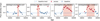 |
Fig. B.1 Examples of flares from the MIRONG sample that do not get selected by our pipeline. The flux density in the W1 band is shown against time. The SDSS designation of the host is shown in the top left corner. |
Appendix C Flares with high angular separation
We calculated the median position of the single-exposure photometry data points for the baseline and the flare data and found 39 objects with a separation of more than 0.5″. This could indicate that the transient is not related to the SMBH in the nucleus of the host.
Three offset flares are the confirmed supernovae discussed in Sect. 3.2.2 and are shown in the top row of Fig. C.1. The second row shows three more flares where the offset looks real which makes them promising supernova candidates.
The first two panels of the last row show objects with an offset where the source of the offset can not be determined. There is no visible host galaxy at the position of the flare in the Pan-STARRS images. J183948+674334 is surrounded by three other sources which could cause the offset although the position of the flare is in between the parent sample galaxy and two of its neighbors.
The remaining objects suffer from a confusion of host galaxies. The third row of Fig. C.1 shows the three objects where the baseline data is associated with the position given by the parent sample. Still, the flare could be associated with a neighboring galaxy. For the 28 remaining offset flares, the opposite is the case. The flare data is more consistent with the parent sample position and the baseline data is skewed towards a neighboring galaxy. An example is shown in the last panel. The confusion is probably due to a host that is too dim in the infrared to generate detections in the single-exposure photometry. The baseline, which is associated with the brighter neighbor is thus too bright causing an underestimation of the flare luminosity.
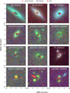 |
Fig. C.1 Pan-STARRS cutouts around the parent sample position of flares with a high angular offset. The red solid cross marks the position of the parent sample galaxy, the black and red circles the position of the single exposure photometry associated with the baseline and the flare, respectively, and the black and red filled cross the respective mean position. |
The 39 brightest mid-IR flares in the catalog, sorted by the maximum flux density in W1 max(vW1 Fw1).
Reasons for rejection of reference sample objects
References
- Aartsen, M. G., Ackermann, M., Adams, J., et al. 2017, Astropart. Phys., 92, 30 [Google Scholar]
- Alexander, T., & Livio, M. 2001, ApJ, 560, L143 [Google Scholar]
- Arcavi, I., Gal-Yam, A., Sullivan, M., et al. 2014, ApJ, 793, 38 [Google Scholar]
- Arcavi, I., McCully, C., Hosseinzadeh, G., et al. 2017, Astron. Telegr., 10668, 1 [Google Scholar]
- Arcavi, I., Burke, J., French, K. D., et al. 2018, Astron. Telegr., 11953, 1 [Google Scholar]
- Astropy Collaboration (Price-Whelan, A. M., et al.) 2022, ApJ, 935, 167 [NASA ADS] [CrossRef] [Google Scholar]
- Baldwin, J. A., Phillips, M. M., & Terlevich, R. 1981, PASP, 93, 5 [Google Scholar]
- Barvainis, R. 1987, Astrophys. J., 320, 537 [Google Scholar]
- Beck, R., Dodds, S. C., & Szapudi, I. 2022, MNRAS 515, 4711 [NASA ADS] [CrossRef] [Google Scholar]
- Beichman, C. A., Neugebauer, G., Habing, H. J., Clegg, P. E., & Chester, T J. 1988, Infrared Astron. Satell. IRAS Cat. Atlases, Vol. 1 Explan. Suppl., 1 [NASA ADS] [Google Scholar]
- Bellm, E. C., Kulkarni, S. R., Graham, M. J., et al. 2018, PASP, 131, 018002 [Google Scholar]
- Berk, D. E. V., Wilhite, B. C., Kron, R. G., et al. 2004, ApJ, 601, 692 [CrossRef] [Google Scholar]
- Bilicki, M., Peacock, J. A., Jarrett, T. H., et al. 2016, ApJS, 225, 5 [Google Scholar]
- Blanchard, P. K., Nicholl, M., Berger, E., et al. 2017, ApJ, 843, 106 [Google Scholar]
- Brescia, M., Cavuoti, S., & Longo, G. 2015, MNRAS, 450, 3893 [NASA ADS] [CrossRef] [Google Scholar]
- Bricman, K., & Gomboc, A. 2020, ApJ, 890, 73 [NASA ADS] [CrossRef] [Google Scholar]
- Brimacombe, J., Stone, G., Masi, G., et al. 2017, Astron. Telegr., 10652, 1 [Google Scholar]
- Chambers, K. C., Magnier, E. A., Metcalfe, N., et al. 2016, ArXiv e-prints [arXiv:1612.05560] [Google Scholar]
- Chan, C.-H., Piran, T., Krolik, J. H., & Saban, D. 2019, ApJ, 881, 113 [Google Scholar]
- Chen, J.-H., Dou, L.-M., & Shen, R.-F. 2022, Astrophys. J., 928, 63 [Google Scholar]
- Chornock, R., Berger, E., Gezari, S., et al. 2013, ApJ, 780, 44 [NASA ADS] [CrossRef] [Google Scholar]
- Cook, D. O., Kasliwal, M. M., Sistine, A. V., et al. 2019, ApJ, 880, 7 [Google Scholar]
- Cook, D. O., Mazzarella, J. M., Helou, G., et al. 2023, ApJS, 268, 14 [NASA ADS] [CrossRef] [Google Scholar]
- Dahiwale, A., & Fremling, C. 2020, Transient Name Serv. Classif. Rep., 2020-1667, 1 [Google Scholar]
- Dálya, G., Galgóczi, G., Dobos, L., et al. 2018, MNRAS, 479, 2374 [Google Scholar]
- Donley, J. L., Brandt, W. N., Eracleous, M., & Boller, T. 2002, AJ, 124, 1308 [NASA ADS] [CrossRef] [Google Scholar]
- Dou, L., Wang, T.-g., Jiang, N., et al. 2016, ApJ, 832, 188 [Google Scholar]
- Draine, B. T., & Lee, H. M. 1984, Astrophys. J., 285, 89 [CrossRef] [Google Scholar]
- Drake, A. J., Djorgovski, S. G., Mahabal, A., et al. 2011, ApJ, 735, 106 [NASA ADS] [CrossRef] [Google Scholar]
- Duncan, K. J. 2022, MNRAS, 512, 3662 [NASA ADS] [CrossRef] [Google Scholar]
- Eddington, A. S. 1913, MNRAS, 73, 359 [Google Scholar]
- Falco, E., Calkins, M., Prieto, J. L., & Stanek, K. Z. 2018, Astron. Telegr., 11180, 1 [Google Scholar]
- Farrar, G. R., & Gruzinov, A. 2009, ApJ, 693, 329 [NASA ADS] [CrossRef] [Google Scholar]
- Flesch, E. W. 2023, Open J. Astrophys., 6, 49 [NASA ADS] [CrossRef] [Google Scholar]
- Foreman-Mackey, D., Hogg, D. W., Lang, D., & Goodman, J. 2013, PASP, 125, 306 [Google Scholar]
- Frederick, S., Gezari, S., Graham, M. J., et al. 2019, ApJ, 883, 31 [Google Scholar]
- Frederick, S., Gezari, S., Graham, M. J., et al. 2021, ApJ, 920, 56 [NASA ADS] [CrossRef] [Google Scholar]
- Fremling, C., & Sharma, Y. 2018, Transient Name Serv. Classif. Rep., 2018-873, 1 [Google Scholar]
- Fremling, C., Dugas, A., & Sharma, Y. 2019, Transient Name Serv. Classif. Rep., 2019-188, 1 [Google Scholar]
- French, K. D., Arcavi, I., & Zabludoff, A. 2016, ApJ, 818, L21 [NASA ADS] [CrossRef] [Google Scholar]
- Gal-Yam, A., Mazzali, P. A., Manulis, I., & Bishop, D. 2013, PASP, 125, 749 [Google Scholar]
- Gezari, S. 2021, Annu. Rev. Astron. Astrophys., 59, 21 [Google Scholar]
- Gezari, S., Martin, D. C., Milliard, B., et al. 2006, ApJ, 653, L25 [Google Scholar]
- Gezari, S., Chornock, R., Rest, A., et al. 2012, Nature, 485, 217 [Google Scholar]
- Gezari, S., Hung, T, Cenko, S. B., et al. 2017, ApJ, 835, 144 [CrossRef] [Google Scholar]
- Graham, M. J., Djorgovski, S. G., Drake, A. J., et al. 2017, MNRAS, 470, 4112 [NASA ADS] [CrossRef] [Google Scholar]
- Hammerstein, E., Gezari, S., van Velzen, S., et al. 2021, Astrophys. J., 908, L20 [Google Scholar]
- Harris, C. R., Millman, K. J., van der Walt, S. J., et al. 2020, Nature, 585, 357 [NASA ADS] [CrossRef] [Google Scholar]
- Hills, J. G. 1975, Nature, 254, 295 [Google Scholar]
- Hinkle, J. T., Holoien, T. W.-S., Auchettl, K., et al. 2021, MNRAS, 500, 1673 [Google Scholar]
- Holoien, T. W.-S., Prieto, J. L., Bersier, D., et al. 2014, MNRAS, 445, 3263 [Google Scholar]
- Holoien, T. W.-S., Neustadt, J. M. M., Vallely, P. J., et al. 2022, ApJ, 933, 196 [NASA ADS] [CrossRef] [Google Scholar]
- Huang, S., Jiang, N., Lin, Z., Zhu, J., & Wang, T. 2023, MNRAS, 525, 4057 [NASA ADS] [CrossRef] [Google Scholar]
- Hunter, J. D. 2007, Comput. Sci. Eng., 9, 90 [NASA ADS] [CrossRef] [Google Scholar]
- Husemann, B., Urrutia, T., Tremblay, G. R., et al. 2016, A&A, 593, L9 [NASA ADS] [CrossRef] [EDP Sciences] [Google Scholar]
- IceCube Collaboration 2013, Science, 342, 1242856 [Google Scholar]
- IceCube Collaboration (FERMI-LAT, MAGIC, et al.) 2018, Science, 361, eaat1378 [NASA ADS] [CrossRef] [Google Scholar]
- Ivezic, Z., Kahn, S. M., Tyson, J. A., et al. 2019, ApJ, 873, 111 [NASA ADS] [CrossRef] [Google Scholar]
- Jarrett, T. H., Cohen, M., Masci, F., et al. 2011, ApJ, 735, 112 [Google Scholar]
- Jiang, N., Zhou, H.-Y., Ho, L. C., et al. 2012, ApJ, 759, L31 [NASA ADS] [CrossRef] [Google Scholar]
- Jiang, N., Dou, L., Wang, T., et al. 2016, Astrophys. J., 828, L14 [Google Scholar]
- Jiang, N., Wang, T., Yan, L., et al. 2017, ApJ, 850, 63 [Google Scholar]
- Jiang, N., Wang, T., Mou, G., et al. 2019, ApJ, 871, 15 [Google Scholar]
- Jiang, N., Wang, T, Dou, L., et al. 2021a, ApJS, 252, 32 [Google Scholar]
- Jiang, N., Wang, T, Hu, X., et al. 2021b, ApJ, 911, 31 [NASA ADS] [CrossRef] [Google Scholar]
- Jiang, N., Zhou, Z., Zhu, J., Wang, Y., & Wang, T. 2023, ApJ, 953, L12 [Google Scholar]
- Kankare, E., Kotak, R., Mattila, S., et al. 2017, Nat. Astron., 1, 865 [NASA ADS] [CrossRef] [Google Scholar]
- Kesden, M. 2012, Phys. Rev. D, 85, 024037 [NASA ADS] [CrossRef] [Google Scholar]
- Kettlety, T, Hesling, J., Phillipps, S., et al. 2018, MNRAS, 473, 776 [NASA ADS] [CrossRef] [Google Scholar]
- Khramtsov, V., Akhmetov, V., & Fedorov, P. 2020, A&A, 644, A69 [EDP Sciences] [Google Scholar]
- Kochanek, C. S. 2016, MNRAS, 461, 371 [NASA ADS] [CrossRef] [Google Scholar]
- Kochanek, C. S., Shappee, B. J., Stanek, K. Z., et al. 2017, PASP, 129, 104502 [Google Scholar]
- Komossa, S. 2015, J. High Energy Astrophys., 7, 148 [Google Scholar]
- Komossa, S., & Greiner, J. 1999, Astron. Astrophys., 349, L45 [Google Scholar]
- Kool, E. C., Reynolds, T. M., Mattila, S., et al. 2020, MNRAS, 498, 2167 [NASA ADS] [CrossRef] [Google Scholar]
- Lacy, M., Ridgway, S. E., Sajina, A., et al. 2015, Astrophys. J., 802, 102 [Google Scholar]
- LaMassa, S. M., Cales, S., Moran, E. C., et al. 2015, ApJ, 800, 144 [NASA ADS] [CrossRef] [Google Scholar]
- Liao, N.-H., Dou, L.-M., Jiang, N., et al. 2019, ApJ, 879, L9 [NASA ADS] [CrossRef] [Google Scholar]
- Lu, W., Kumar, P., & Evans, N. J. II 2016, MNRAS, 458, 575 [Google Scholar]
- Lynden-Bell, D. 1969, Nature, 223, 690 [NASA ADS] [CrossRef] [Google Scholar]
- Madau, P, & Dickinson, M. 2014, Ann. Rev. Astron. Astrophys., 52, 415 [Google Scholar]
- Magorrian, J., Tremaine, S., Richstone, D., et al. 1998, AJ, 115, 2285 [Google Scholar]
- Mainzer, A., Bauer, J., Cutri, R. M., et al. 2014, ApJ, 792, 30 [Google Scholar]
- Malyali, A., Rau, A., Merloni, A., et al. 2021, A&A, 647, A9 [NASA ADS] [CrossRef] [EDP Sciences] [Google Scholar]
- Masterson, M., De, K., Panagiotou, C., et al. 2024, ApJ, 961, 211 [NASA ADS] [CrossRef] [Google Scholar]
- Mattila, S., Pérez-Torres, M., Efstathiou, A., et al. 2018, Science, 361, 482 [Google Scholar]
- McInnes, L., & Healy, J. 2017, in 2017 IEEE Int. Conf. Data Min. Workshop ICDMW, 33 [Google Scholar]
- McKinney, W. 2010, Proc. 9th Python Sci. Conf., 56 [Google Scholar]
- Mockler, B., Guillochon, J., & Ramirez-Ruiz, E. 2019, ApJ, 872, 151 [Google Scholar]
- Necker, J. 2024, https://zenodo.org/records/114462 50 [Google Scholar]
- Necker, J., & Mechbal, S. 2024, https://zenodo.org/records/10473347 [Google Scholar]
- Necker, J., de Jaeger, T., Stein, R., et al. 2022, MNRAS, 516, 2455 [NASA ADS] [CrossRef] [Google Scholar]
- Necker, J., IceCube, Abbasi, R., et al. 2023, in Proc. 38th Int. Cosm. Ray Conf. — PoSICRC2023, 444 (SISSA Medialab), 1478 [Google Scholar]
- Neustadt, J. M. M., Holoien, T. W.-S., Kochanek, C. S., et al. 2020, MNRAS, 494, 2538 [Google Scholar]
- Nicholl, M., Blanchard, P. K., Berger, E., et al. 2019, MNRAS, 488, 1878 [NASA ADS] [CrossRef] [Google Scholar]
- Nordin, J., Brinnel, V., van Santen, J., et al. 2019, A&A, 631, A147 [NASA ADS] [CrossRef] [EDP Sciences] [Google Scholar]
- Ochmann, M. W., Kollatschny, W., Probst, M. A., et al. 2024, The Transient Event in NGC 1566 from 2017 to 2019. I. An Eccentric Accretion Disk and a Turbulent, Disk-Dominated Broad-Line Region Unveiled by Double-Peaked Ca II and O I Lines [Google Scholar]
- Panagiotou, C., De, K., Masterson, M., et al. 2023, Astrophys. J., 948, L5 [Google Scholar]
- Pedregosa, F., Varoquaux, G., Gramfort, A., et al. 2011, J. Mach. Learn. Res., 12, 2825 [Google Scholar]
- Petrushevska, T., Leloudas, G., Ilić, D., et al. 2023, A&A, 669, A140 [NASA ADS] [CrossRef] [EDP Sciences] [Google Scholar]
- Pitik, T., Tamborra, I., Angus, C. R., & Auchettl, K. 2022, ApJ, 929, 163 [NASA ADS] [CrossRef] [Google Scholar]
- Pitik, T, Tamborra, I., Lincetto, M., & Franckowiak, A. 2023, MNRAS, 524, 3366 [NASA ADS] [CrossRef] [Google Scholar]
- Planck Collaboration VI. 2020, A&A, 641, A6 [NASA ADS] [CrossRef] [EDP Sciences] [Google Scholar]
- Rees, M. J. 1984, Annu. Rev. Astron. Astrophys., 22, 471 [Google Scholar]
- Rees, M. J. 1988, Nature, 333, 523 [Google Scholar]
- Reguitti, A. 2022, Transient Name Serv. Classif. Rep., 2022-3144, 1 [Google Scholar]
- Reines, A. E., & Volonteri, M. 2015, ApJ, 813, 82 [NASA ADS] [CrossRef] [Google Scholar]
- Reusch, S., Stein, R., Kowalski, M., et al. 2022, Phys. Rev. Lett., 128, 221101 [NASA ADS] [CrossRef] [Google Scholar]
- Reynolds, T. M., Mattila, S., Efstathiou, A., et al. 2022, A&A, 664, A158 [NASA ADS] [CrossRef] [EDP Sciences] [Google Scholar]
- Ryu, T., McKernan, B., Ford, K. E. S., et al. 2024, MNRAS, 527, 8103 [Google Scholar]
- Sagiv, I., Gal-Yam, A., Ofek, E. O., et al. 2014, AJ, 147, 79 [NASA ADS] [CrossRef] [Google Scholar]
- Scargle, J. D., Norris, J. P., Jackson, B., & Chiang, J. 2013, ApJ, 764, 167 [Google Scholar]
- Sokal, A. 1997, in Functional Integration: Basics and Applications, eds. C. DeWitt-Morette, P. Cartier, & A. Folacci, NATO ASI Series (Boston, MA: Springer US), 131 [Google Scholar]
- Somalwar, J. J., Ravi, V., Yao, Y., et al. 2023, arXiv e-prints [arXiv:2310.03782] [Google Scholar]
- Stern, D., Assef, R. J., Benford, D. J., et al. 2012, ApJ, 753, 30 [Google Scholar]
- Stein, R., van Velzen, S., Kowalski, M., et al. 2021, Nat. Astron., 5, 510 [NASA ADS] [CrossRef] [Google Scholar]
- Stein, R., Reusch, S., Franckowiak, A., et al. 2023, MNRAS, 521, 5046 [CrossRef] [Google Scholar]
- Sun, H., Zhang, B., & Li, Z. 2015, ApJ, 812, 33 [NASA ADS] [CrossRef] [Google Scholar]
- Tadhunter, C., Spence, R., Rose, M., Mullaney, J., & Crowther, P. 2017, Nat. Astron., 1, 1 [Google Scholar]
- Thévenot, M., Gantier, J. M., Kabatnik, M., Schümann, J., & Gramaize, L. 2021a, Res. Notes AAS, 5, 58 [Google Scholar]
- Thévenot, M., Kabatnik, M., & Gantier, J. M. 2021b, Transient Name Serv. AstroNote, 212, 1 [Google Scholar]
- Tinyanont, S., Kasliwal, M. M., Fox, O. D., et al. 2016, ApJ, 833, 231 [NASA ADS] [CrossRef] [Google Scholar]
- Trakhtenbrot, B., Arcavi, I., Ricci, C., et al. 2019, Nat. Astron., 3, 242 [Google Scholar]
- Tucker, M. A. 2021, Transient Name Serv. Classif. Rep., 2021-433, 1 [Google Scholar]
- Ulmer, A. 1999, ApJ, 514, 180 [Google Scholar]
- Ulrich, M.-H., Maraschi, L., & Urry, C. M. 1997, Annu. Rev. Astron. Astrophys., 35, 445 [Google Scholar]
- van Velzen, S., Farrar, G. R., Gezari, S., et al. 2011, ApJ, 741, 73 [Google Scholar]
- van Velzen, S., Mendez, A. J., Krolik, J. H., & Gorjian, V. 2016, ApJ, 829, 19 [NASA ADS] [CrossRef] [Google Scholar]
- van Velzen, S., Gezari, S., Hammerstein, E., et al. 2021, ApJ, 908, 4 [NASA ADS] [CrossRef] [Google Scholar]
- van Velzen, S., Stein, R., Gilfanov, M., et al. 2024, MNRAS, 529, 2559 [CrossRef] [Google Scholar]
- Veres, P. M., Franckowiak, A., van Velzen, S., et al. 2024, arXiv e-prints [arXiv:2408.17419] [Google Scholar]
- Virtanen, P., Gommers, R., Oliphant, T. E., et al. 2020, Nat. Methods, 17, 261 [Google Scholar]
- Wang, T, Yan, L., Dou, L., et al. 2018, MNRAS, 477, 2943 [NASA ADS] [CrossRef] [Google Scholar]
- Wang, Y., Jiang, N., Wang, T., et al. 2022a, ApJS, 258, 21 [Google Scholar]
- Wang, Y., Jiang, N., Wang, T., et al. 2022b, ApJ, 930, L4 [NASA ADS] [CrossRef] [Google Scholar]
- Wang, Y., Wang, T., Jiang, N., et al. 2024, arXiv e-prints [arXiv:2312.12015] [Google Scholar]
- Wang, Y., Baldi, R. D., del Palacio, S., et al. 2023, MNRAS, 520, 2417 [NASA ADS] [CrossRef] [Google Scholar]
- Wen, S., Jonker, P. G., Stone, N. C., Zabludoff, A. I., & Cao, Z. 2022, ApJ, 933, 31 [NASA ADS] [CrossRef] [Google Scholar]
- Wevers, T., Coughlin, E. R., Pasham, D. R., et al. 2023, ApJ, 942, L33 [NASA ADS] [CrossRef] [Google Scholar]
- Wild, V, Almaini, O., Dunlop, J., et al. 2016, MNRAS, 463, 832 [NASA ADS] [CrossRef] [Google Scholar]
- Yang, Q., Green, P. J., MacLeod, C. L., et al. 2023, ApJ, 953, 61 [NASA ADS] [CrossRef] [Google Scholar]
- Yao, Y., Ravi, V., Gezari, S., et al. 2023, ApJ, 955, L6 [NASA ADS] [CrossRef] [Google Scholar]
- Zhang, X., Wang, X., Sai, H., et al. 2022, MNRAS, 509, 2013 [Google Scholar]
Luminosity functions were derived from observations of the Spitzer Space Telescope but only for AGNs (Lacy et al. 2015).
All Tables
Absolute and relative numbers of the results of our pipeline for three reference samples
The 39 brightest mid-IR flares in the catalog, sorted by the maximum flux density in W1 max(vW1 Fw1).
All Figures
|
Fig. 1 Flowchart of the flare selection process. See Sect. 2.3 for a detailed explanation of the selection steps. |
| In the text | |
|
Fig. 2 Representative examples of the classification of the pipeline outlined in Fig. 1 for steps 3 (WISEA J063233+655809), 5 (WISEA J105052+000134), and 10 (WISEA J144620+371159) from left to right detailed in Sect. 2.3, which impact the completeness (see Sect. 4). The last panel shows one example of a dust echo-like flare (WISEA J083416-054249). The flux density in the W1 band is shown against time. The classification is annotated in the upper left corner. |
| In the text | |
|
Fig. 3 Blackbody fits for NGC 7392 for all epochs of the flare where the MCMC sampling resulted in meaningful constraints on the fit parameters. The dashed green line shows the best fit and the transparent lines show the results from the MCMC sampling. The best fit and 68th percentile temperature and effective radius values are shown in the bottom left corner. The frequency, v, is given in the source frame. |
| In the text | |
|
Fig. 4 Light curve and evolution of Reff and T for NGC 7392. The crosses mark the best-fit values of the visit where the MCMC sampling did not result in a meaningful constraint of Lbol . The results are consistent with Panagiotou et al. (2023). |
| In the text | |
|
Fig. 5 Parameters from the blackbody fits for 449 sources where at least two epochs have a good fit. The time is given in the source frame. First panel: Bolometric flux based on the bolometric luminosity and the luminosity distance. Second panel: Bolometric luminosity (see Eq. (7)). Third and fourth panel: Temperature and effective radius (see Eq. (6)). |
| In the text | |
|
Fig. 6 Distribution of the total emitted energy, assuming hot dust (Eq. (8)). The quasars are identified by a match to Milliquas (see Sect. 3.1). |
| In the text | |
|
Fig. 7 Dust radius estimated from the IR light curve, RLC, against the radius at the peak, Reff,peak, obtained from the blackbody fits. The colored contours represent the actual blackbody radius for a finite width of the initial O/UV transient (see Eq. (11)). |
| In the text | |
|
Fig. 8 Correlation of the total emitted bolometric energy Ebol, the peak bolometric luminosity Lbol,peak and the dust radius infered from the light curve RLC. The dashed lines represent the theoretically expected relations. |
| In the text | |
|
Fig. 9 Distribution of peak dates over time. The reference time window from around May 2016 to June 2020 is indicated as the grey-shaded region. The break of WISE data taking is indicated with grey dashed lines. |
| In the text | |
|
Fig. 10 Rate as a function of the absolute magnitude in W1 and redshift. The light blue histogram shows the total number of galaxies in the parent galaxy sample and the green one is the host of our flare sample. The black hatched bars represent flares with Lbol,peak < 6 × 1043 erg. The grey data points and black errors show the rate as calculated with Eq. (12). The grey triangles are the 90% upper limit on the rate where no flare was observed. The errors are statistical only. |
| In the text | |
|
Fig. 11 Distribution of the maximum bolometric luminosity as a function of redshift. |
| In the text | |
|
Fig. 12 Evolution of the rate with redshift for the two MW1 bins where there are flares in the first and at least one other redshift bin, normalized to the first redshift bin. Open symbols represent upper limits. The redshift evolution of the star formation rate (SFR) Madau & Dickinson (2014) and for TDEs Sun et al. (2015) is shown for comparison. |
| In the text | |
|
Fig. B.1 Examples of flares from the MIRONG sample that do not get selected by our pipeline. The flux density in the W1 band is shown against time. The SDSS designation of the host is shown in the top left corner. |
| In the text | |
|
Fig. C.1 Pan-STARRS cutouts around the parent sample position of flares with a high angular offset. The red solid cross marks the position of the parent sample galaxy, the black and red circles the position of the single exposure photometry associated with the baseline and the flare, respectively, and the black and red filled cross the respective mean position. |
| In the text | |
Current usage metrics show cumulative count of Article Views (full-text article views including HTML views, PDF and ePub downloads, according to the available data) and Abstracts Views on Vision4Press platform.
Data correspond to usage on the plateform after 2015. The current usage metrics is available 48-96 hours after online publication and is updated daily on week days.
Initial download of the metrics may take a while.