| Issue |
A&A
Volume 695, March 2025
|
|
|---|---|---|
| Article Number | A13 | |
| Number of page(s) | 13 | |
| Section | Catalogs and data | |
| DOI | https://doi.org/10.1051/0004-6361/202451298 | |
| Published online | 27 February 2025 | |
Substellar candidates at the earliest stages: The SUCANES database
1
ISDEFE
Beatriz de Bobadilla 3,
28040
Madrid,
Spain
2
Centro de Astrobiología (CAB), CSIC-INTA,
ESAC Campus, Camino bajo del Castillo s/n,
28692
Villanueva de la Cañada, Madrid,
Spain
3
European Space Agency, ESAC, Camino Bajo del Castillo,
28692
Villanueva de la Cañada, Madrid,
Spain
4
Universidad Nacional Autónoma de México, Instituto de Radioastronomía y Astrofísica,
Antigua Carretera a Pátzcuaro 8701, Ex-Hda. San José de la Huerta,
58089
Morelia,
Michoacán,
Mexico
5
European Southern Observatory,
Alonso de Cordova 3107, Casilla 19,
Vitacura, Santiago,
Chile
6
Institut de Ciències de l’Espai (ICE-CSIC),
Campus UAB, Can Magrans S/N,
08193
Cerdanyola del Vallès,
Spain
7
European Southern Observatory,
Karl-Schwarzschild-Strasse 2,
85748
Garching bei München,
Germany
8
Laboratoire d’Astrophysique de Bordeaux, Univ. Bordeaux, CNRS,
B18N, allée Geoffroy Saint-Hilaire,
33615
Pessac,
France
★ Corresponding author; This email address is being protected from spambots. You need JavaScript enabled to view it.
Received:
28
June
2024
Accepted:
19
December
2024
Abstract
Context. Brown dwarfs are the bridge between low-mass stars and giant planets. One way of shedding light on their dominant formation mechanism is to study them at the earliest stages of their evolution, when they are deeply embedded in their parental clouds. Several works have identified pre- and proto-brown dwarf candidates using different observational approaches.
Aims. The aim of this work is to create a database of all the objects classified as very young substellar candidates in the literature in order to study them homogeneously.
Methods. We gathered all the information about very young substellar candidates available in the literature until 2020. We retrieved their published photometry from the optical to the centimetre regime, and we wrote our own codes to derive their bolometric temperatures and luminosities, and their internal luminosities. We also populated the database with other parameters extracted from the literature, such as the envelope masses, their detection in some molecular species, and the presence of outflows.
Results. The result of our search is the SUbstellar CANdidates at the Earliest Stages (SUCANES) database, containing 174 objects classified as potential very young substellar candidates in the literature. We present an analysis of the main properties of the retrieved objects. Since we updated the distances to several star forming regions, we were able to reject some candidates based on their internal luminosities. We also discuss the derived physical parameters and envelope masses for the best substellar candidates isolated in SUCANES. As an example of a scientific exploitation of this database, we present a feasibility study for the detection of radio jets with upcoming facilities: the next generation Very Large Array and the Square Kilometer Array interferometers. The SUCANES database is accessible through a graphical user interface, and it is open to any potential user.
Key words: astronomical databases: miscellaneous / brown dwarfs / stars: low-mass / stars: protostars
© The Authors 2025
 Open Access article, published by EDP Sciences, under the terms of the Creative Commons Attribution License (https://creativecommons.org/licenses/by/4.0), which permits unrestricted use, distribution, and reproduction in any medium, provided the original work is properly cited.
This article is published in open access under the Subscribe to Open model. This email address is being protected from spambots. You need JavaScript enabled to view it. to support open access publication.
1 Introduction
Brown dwarfs (BDs) are substellar objects with masses from ~80−13 MJup, so they are the bridge between low-mass stars and Jupiter-like planets. A large number of observational works (e.g. Natta et al. 2002; Whelan et al. 2005; Barrado y Navascués et al. 2007; Alves de Oliveira et al. 2010; Bayo et al. 2012; Mužić et al. 2014) have shown that young BDs (~1−10 Myr) share properties with young low-mass stars, such as the presence of discs and jets, suggesting that they share the same formation mechanism. However, since their discovery, the formation of BDs has been under debate, with the aim of understanding the dominant mechanism of substellar formation. The most widely discussed mechanisms are turbulent fragmentation (Padoan & Nordlund 2004; Hennebelle & Chabrier 2008), ejection from multiple pro-tostellar systems (Reipurth & Clarke 2001; Bate 2012), highly erosive outflows (Machida et al. 2009), and disc fragmentation (Whitworth & Stamatellos 2006). In the surroundings of high-mass stars, there are additional mechanisms that might form BDs, namely the photo-evaporation of cores near massive stars (Whitworth & Zinnecker 2004) and gravitational fragmentation of dense filaments formed in a nascent cluster (Bonnell et al. 2008).
Since stars and BDs evolve very rapidly during the first million years, one way to shed light on the dominant BD formation scenario is to study the properties of BDs at the earliest stages of their evolution, when they are still embedded in the parental clouds. If BDs are a scaled-down version of low-mass stars, they are expected to form in isolation within molecular clouds with the same observational properties and correlations in physical parameters as those found in protostars (e.g. envelopes, molecular outflows, or thermal radiojets). By analogy with low-mass stars, BDs would be expected to show different evolutionary stages characterised by different physical and morphological properties and spectral energy distributions (SEDs; see Lada & Wilking 1984; Lada 1987; Andre et al. 1993); in the earliest phases, we would find the pre-BDs, which are dense cores that will form a BD in the future but have not formed a hydrostatic core yet (i.e. it is an analog to the pre-stellar cores for low-mass stars). Class 0 proto-BDs would consist of embedded cold cores with SEDs peaking at the (sub-)millimetre regime, while Class I proto-BDs should be characterized by an infalling envelope feeding an accreting circumstellar disc and with SEDs peaking in the far-infrared.
From an observational point of view, several efforts have been made to identify the youngest BDs. In the early 2000s, the Spitzer Space Telescope identified a new family of objects called very low-luminosity objects (VeLLOs Young et al. 2004; di Francesco et al. 2007), which were recognised as potential proto-BDs. They are deeply embedded objects characterised by internal luminosities1 (Lint) below 0.1–0.2 L⊙ (Dunham et al. 2008; Kim et al. 2016). A number of these VeLLOs have been further characterised (e.g. Bourke et al. 2006; Dunham et al. 2008; Palau et al. 2012, 2014; Morata et al. 2015; Kim et al. 2016, 2019) using different observations and display properties consistent with proto-BDs.
Another group of objects with very low internal luminosities are the so-called first hydrostatic cores (FHCs). They are supposed to form during the first stages of collapse, once the density is large enough to turn the collapse from isothermal to adiabatic, providing the required pressure to balance gravity. The predicted properties of FHCs are low internal luminosities, very low accreted masses, SEDs peaking around 100 µm, and an association with low-velocity outflows. Thus, the properties of FHCs are similar to the properties expected for deeply embedded Class 0-like proto-BDs. The mass reservoir in the envelope is the key distinguishing parameter between the two: for an FHC to end up as a substellar object, the mass of the envelope should be low enough to guarantee that the accreted material does not place the object in the stellar regime. Only a few FHC candidates have been identified so far (see e.g. Palau et al. 2014; Hirano 2019; Maureira et al. 2020).
Pre-brown-dwarf (pre-BD) cores are also potential substellar objects: they are cores detected mainly at continuum (sub-)mm wavelengths with no infrared or optical counterparts, and with Lint upper limits <0.2 L⊙; they are gravitationally bound, but have very low masses (near substellar); thus, they will not be able to form a stellar object, even if accreting all the reservoir of mass within the core. So far, there is only one well-characterised pre-BD (André et al. 2012) and several candidates (e.g. Palau et al. 2012; de Gregorio-Monsalvo et al. 2016; Huélamo et al. 2017; Santamaría-Miranda et al. 2021).
Several studies have identified substellar candidates at very early stages of their formation (FHCs, pre- and proto-BDs) in star-forming regions using different observational approaches. A comprehensive study comparing the properties of all the candidates homogeneously is needed in order to shed light on their formation mechanism. In this context, and as a first step, we created the SUbstellar CANdidates at the Earliest Stages (SUCANES) database (DB); it is intended to be a compilation of all the sources that have been identified as probable pre-BD, proto-BD, VeLLO, and FHC candidates in the literature. The SUCANES DB is accessible through a graphical user interface (GUI) and is open to any potential user.
In this manuscript, we describe how we built SUCANES and collected the data used to populate it, and we include a brief analysis of its contents. A description of the sample selection and the data used in the DB are described in Sect. 2, while the GUI used to access the DB is described in Sect. 3. A summary of the main properties of the compiled objects is presented in Sect. 4. Finally, we include a scientific application of the DB in Sect. 5. Our main conclusions are summarised in the last section of this paper.
2 The SUCANES database
The SUCANES DB was built using data from the literature published up to and including 2020 and is complemented with photometry from public archives and catalogues (from VizieR). The objects that populate SUCANES are those with the following properties:
Published works have classified them as pre- or proto-BDs.
Published works have classified them as VeLLOs, that is, young objects with low internal luminosities (Lint < 0.2 L⊙, within the errors).
Objects classified as FHCs.
All the objects selected above show Class 0, 0/I, I, Flat, or an unknown class; that is, we do not include Class II objects.
The SUCANES database was constructed in a MariaDB2 system using Python scripts. The database was built creating different tables (in csv format) including different information about the targets. All these tables are connected by a common object identification number (ObjID).
The DB contains a total of 11 tables that can be grouped in four different blocks: identification tables (2), photometric tables (6), physical-parameter tables (2), and molecular line-emission table (1). We describe all these tables and the information contained in each of them in the following subsections and in Appendix A. We note that all the SUCANES material is available in the GitHub repository3.
2.1 SUCANES identification tables
The first two tables of SUCANES are the identification tables (Identity and Position), which contain the following basic information about the objects:
Identity includes two columns, including Name, for the name of the object as found in the literature, and Other Name, which is a resolver ID that facilitates archival searches. For this second column, we used sesame resolvable IDs whenever available4 and the ViZieR association when the former did not exist.
Position includes the object coordinates, RA(J2000) and DEC(J2000), the star forming region they belong to (Region), their distance (in pc), their Class and Type, and the corresponding bibliographic references from which all the information, including the Name from the Identity table, was extracted.
We have considered updated distances to different star forming regions following the results from works using mainly Gaia and Very Long Baseline Array (VLBA) data (see Table 1 for the corresponding references). We adopted new distance values to Perseus, IC348, Serpens, Aquila, GF 9, Corona Australis, and σ Orionis. In the case of Ophiuchus objects, we adopted different values for objects in the L 1689 and L 1688 clouds. IC 5146 has been studied by Wang et al. (2020), concluding that the region has two components: the Cocoon Nebula and the filaments. After checking that all the objects in SUCANES lie in the filaments, we adopted a distance of 600±100 pc. In the case of Cepheus, we compared the location of the nine objects included in SUCANES within the groups defined by Szilágyi et al. (2021): three lie in the NGC 7023, and four in L 1251. One of the objects (J215607) lies close to the latter region, but outside the area defined in that work. Hence, we included ‘Cepheus/L1251?’ in its ‘Region’ field, while the ninth object lies in the L1148 cloud. Finally, for Chamaeleon we adopted different distances for the I, II, and III clouds. For the rest of the regions, we used the distances quoted in the different publications: some of them have already been estimated using Gaia data (e.g. Lupus, Santamaría-Miranda et al. 2021) or are consistent with those reported in recent studies including Gaia data (e.g. Taurus, Orion, California; see Galli et al. 2019; Zucker et al. 2020).
The Class column refers to the evolutionary class of the objects (see e.g. Lada & Wilking 1984; Lada 1987). This class has traditionally been estimated measuring the slope (αIR) of the SED in the infrared range (normally from 2 to 10–25 µm), so that the objects follow an evolutionary sequence covering several classes: I, Flat, II, and III. An earlier class (Class 0) was defined later by Andre et al. (1993) based on different criteria. Another approach to derive the evolutionary stage of a young stellar object is to use the bolometric temperature (Tbol) that comes from the SED (see Sect. 2.3). The connection between the Tbol value and the classes was first done by Chen et al. (1995), and later revised by Evans et al. (2009). SUCANES includes objects with classes between 0 and Flat that were retrieved from the literature. Since we are studying embedded objects, the class was always derived using the Tbol value. In the particular case of Kim et al. (2016), a Tbol value was estimated for the sources, but they did not explicitly mention a class. In those cases, we assigned a value using the quoted Tbol and followed the prescription by Chen et al. (1995). Finally, we note that the objects classified as pre-BD or FHC candidates are objects less evolved than Class 0 ones, so they are not within the classification scheme described above. In these cases, we filled the Class field with N.A.
The Type column refers to the classification of the objects in the literature, and its value can be ‘proto-BD’, ‘pre-BD’, ‘FHC’, or ‘VeLLO’. In three cases, we also include the type ‘protostar’, since the nature of the object is under discussion. It is important to remark that, regardless of this classification, all the objects in SUCANES should be considered as substellar candidates as there are no unambiguous observations that have confirmed them as pre- or proto-BDs yet. A brief discussion of individual objects whose nature is not clear is included in Appendix C.
Finally, we note that we include a ‘D’ after the type (e.g. VeLLO/D and proto-BD/D) to indicate objects discarded as young substellar candidates after our own analysis presented here. They are mainly discarded after the recalculation of the internal luminosities using updated distances (see Sect. 4.1) or due to other findings described below such as new Euclid data indicating that a source is extragalactic (Bouy et al., in prep.).
Adopted distances for different regions in SUCANES.
2.2 SUCANES photometric tables
The SUCANES DB contains photometric information (continuum data) of the objects from the optical to the centimetre range. We created a total of six tables with the following information:
Optical: photometry in RIZ-filters. The table includes the measured magnitudes and the instrumentation used.
NIR: photometry in the JHKs filters. The table includes the measured magnitudes and the instrumentation used.
Spitzer: photometric data obtained with the IRAC & MIPS instruments onboard the Spitzer space telescope. We note that we only considered Spitzer and not WISE data for the 3–24 µm wavelength range, given the better angular resolution of the former.
Herschel: photometric data obtained with the PACS & SPIRE instruments onboard the Herschel telescope.
Sub-millimetre: sub-millimetre continuum fluxes. It was built using published data from single-dish and interferometer facilities. It is the most inhomogeneous table, in the sense that contains data covering a broad wavelength range (from 350 µm to 7.3 mm) obtained at very different angular resolutions. To provide as much information as possible, the table includes the observing wavelength, the flux density used to build the SED, the peak intensity and the integrated flux, the size and position angle (PA) of the beam, the angular size and PA of the source, and the name of the interferometer (or antenna) where the data was obtained. We also include the flag Resolved, which adopts a value of 0 if the object is not spatially resolved, and a value of 1 if it is resolved.
Centimetre: data in the centimetre regime, from 1 cm long-wards. The contents of the table are similar to the sub-millimetre one, and it is populated mainly with interferometric data from the Jansky Very Large Array (JVLA). In this table, we include an additional flag called Variability, which provides information on the source variability at 8.5 GHz (3.5 cm). We populated this column with the results of Choi et al. (2014), which studied the centimetre variability of ten VeLLOs. If there is information about the source variability, it adopts a value of 1, and if there is not information a value of 0.
The optical and near-IR photometry are provided in Vega magnitudes, while the rest of the fluxes are provided in millijanskys. For clarity, we built an auxiliary table (named Filters) with the filters used to obtain the photometric data, including the corresponding zero points to change from magnitudes to fluxes, or vice versa5. All the magnitudes and fluxes have an associated error. Whenever this error value is equal to 0.0, the corresponding magnitude or flux is an upper limit. We note that all the photometric tables include a column with the bibliographic references from which the data were retrieved. We provide a detailed description of the contents of each photometric table in Appendix A.
2.3 SUCANES physical-parameter tables
The SUCANES DB includes two tables with physical parameters of the sources: LumTbol and Dust_properties. The first table contains information about the internal luminosity (Lint), bolometric luminosity (Lbol), and bolometric temperature (Tbol) of the objects, and the second table includes information about the dust mass (Mdust) and total mass (gas+dust, Mtotal) of the envelopes around the objects. While we derived the parameters included in the first table using the retrieved photometry and our own codes implemented in the DB, the second table is populated with data from the literature. We now describe their contents. For the LumTbol table, we estimated the physical parameters of the objects in the following way:
-
Internal Luminosity: the internal luminosity is defined as the total luminosity arising from a central object and its disc (including both accretion and photospheric luminosity) and excluding any luminosity arising from external heating of the surrounding dense core by the interstellar radiation field. The internal luminosity (in units of solar luminosity) is estimated using the flux at 70 µm (from PACS@Herschel or MIPS@Spitzer) and the distance to the source, D in pc, adapting the following prescription by Dunham et al. (2008):
![Mathematical equation: ${L_{{\rm{int }}}}\left( {{L_ \odot }} \right) = 3.3 \times {10^8} \cdot {\left[ {{F_{70}} \times {{(D/140)}^2}} \right]^{0.94}},$](/articles/aa/full_html/2025/03/aa51298-24/aa51298-24-eq1.png) (1)
(1)where F70 corresponds to λ⋅Fλ in erg/s/cm2.
Given the better sensitivity and angular resolution of the Herschel/PACS data in comparison with Spitzer/MIPS, we always consider the former to derive Lint if both fluxes are available.
Dunham et al. (2008) considered VeLLOs as objects with Lint ≤0.1 L⊙. However, other works have relaxed this limit to 0.2 L⊙ to take into account an uncertainty of factor of ~2 associated with the Lint estimation from the 70 µm flux using Eq. (1) (see Kim et al. 2016). We adopted this latter approximation and considered VeLLOs as those that fulfill that their Lintis ≤ 0.2L⊙ within the errors: that is, Lint – errLint ≤ 0.2 L⊙. We discuss the distribution of internal luminosities in detail in Sect. 4.
Bolometric luminosity: The Lbol of any source in SUCANES was estimated by integrating its SED from the optical to the millimetre range including detections and upper limits and then using its distance (D) to convert the flux into a luminosity. To calculate Lbol, we imposed that the object should be detected in at least three different wavelength ranges (i.e. three different photometric tables) to ensure a significant spectral coverage. If the object does not fulfil this condition, the bolometric luminosity is not computed.
-
Bolometric temperature: The Tbol of an object with an spectrum Fν is defined as the temperature of a blackbody whose spectrum has the same mean frequency (
 ) as the observed spectrum (Myers & Ladd 1993) and can be derived using the following expression:
 (2)
(2)where
 is defined as the ratio of the first and the zeroth frequency moments of the spectrum (Ladd et al. 1991):
 (3)
(3)Basically,
 provides a measurement of the redness of a given SED. As in the case of Lbol, it is necessary for the object to show detections in three different photometric tables to compute the bolometric temperature. Both Lbol and Tbol are estimated with a simple numerical integration using photometric points from the optical to the sub-millimetre range.
The second table of the DB with physical parameters, Dust_properties, contains the estimated envelope masses (dust and dust+gas masses) of the objects, as quoted in the literature. We also include the bibliographic reference from which these masses were adopted.
The values of the envelope dust masses in the literature were mainly estimated from a given (sub-)millimetre-continuum flux density (Sλ) at a given wavelength assuming optically thin conditions and following the equation
 (4)
(4)
where D is the distance to the source (in pc), Bλ is the Planck function, Tdust is the dust temperature in kelvin, and κλ is the opacity per dust+gas mass (in cm2/g) at the observing wavelength. We note that this value is normally estimated by the interpolation of dust opacities from theoretical models (Ossenkopf& Henning 1994). For completeness, we include the dust temperature and the opacity used for the mass estimation in the table, as quoted in the corresponding publication. In addition, we include the observing wavelength and a field called Beam, which is the observational beam size and useful for understanding if the mass estimation comes from a single dish (single value) or interferometric observations (synthesised beam size in XY). We note that for the objects with revised distances, we recalculated the published masses using the new distance values.
For a few objects, the masses were estimated either by modelling the SED (e.g. ObjID 3) or using a particular model for the envelope (e.g. ObjID 204). In these cases, we add a note in the ‘Publication’ field with this information, and we only include the Tdust and the dust mass resulting from the fit in the table, without providing a particular wavelength or beam size for the observations (the value None is included in those two fields).
The total (gas+dust) masses in SUCANES are simply estimated from the dust mass and assuming a gas-to-dust mass ratio of 100, so Mtotal = 100 × Mdust. They are expressed in M⊙. The contents of the two tables including the derived Lint, Lbol, Tbol and the adopted Mdust & Mtotal are described in Appendix A.
2.4 SUCANES molecular line-emission table
While continuum observations of very young substellar objects provide information about their dust content, the observations in different gas molecules are relevant to further characterising the objects, revealing important properties such as the presence of molecular outflows, their chemical composition, or their belonging to a particular star forming region by analysing their systemic velocities.
A large fraction of SUCANES objects have observations in molecular spectral lines. Since these observations are very inhomogeneous (e.g. different antennas or interferometers, molecular transitions), we constructed a table providing information about the availability of gas observations without providing fluxes. The table contains a list of gas molecules frequently observed when studying embedded objects, together with the bibliographic references where these molecules have been presented. For each molecule, we include a value of 0 if no data are available and 1 if there are data, regardless of the detection or non-detection of the object. In particular, we include information about the availability of CO, C, HCN, HCO+, N2H+, CS, CN, CH3OH, and SiO. The particular transition for each molecule should be checked in the publications provided in the pub_mol column.
In addition to the studied molecules, we also provide information on the presence of molecular outflows (1 for detected, 0 for non-detected, and None if no data are available) associated with the objects and the molecule used for the study. The bibliographic references from which these data were retrieved are included in the last column. A detailed description of this table can be found in Appendix A.
3 The SUCANES GUI
Access to SUCANES by any external user can be gained through a GUI on the public web page6. The SUCANES GUI allows any user to create queries, download the requested information in csv files, and plot the data in different graphs. In fact, any user can have access to all the data and physical parameters described in Sect. 2 through this GUI, allowing them to retrieve all the information contained in the eleven SUCANES tables in a single csv table.
In brief, users can query the GUI using the search button at the top of the page. Searches can be done using the name of an object (or part of it), the coordinates, and (or) an object type (e.g. proto-BD, pre-BD); that is, the user can select only by name, only by coordinates (RA and Dec in degrees), or only by type, or by using both name and type, or both coordinates and type. The only combination that is not allowed is name and coordinates. The output of a query, if there are objects in SUCANES that fulfill the search inputs, is an html table showing basic information about the object(s): name, celestial coordinates, sky region, type, and class. In addition, a Boolean column (molecular emission) indicates if the object has been observed in any molecular transition. The user can also plot the SED of any of the objects in this table by clicking on the sed button located at the end of the row of each object. The SED is represented with the X-axis displaying the wavelength (in microns) and the Y-axis the flux density (in mJy), showing all the available data from the optical to the centimetre range.
For any selected object, the user can download all the available data from SUCANES in a csv file, which will contain basic information about the object, the photometry to build the SED, the estimated envelope masses, and the derived Lint, Lbol, and Tbol parameters. An additional column will indicate if the object is included in the SUCANES molecular line-emission table. The file can be retrieved by clicking on the Photometry button located in the top right of the web page.
Finally, we note that if the users are interested in downloading the whole database, they can do so by selecting ‘ALL’ in the Types field, clicking ‘search’, and then clicking on the Photometry button. As a result, the user will obtain a csv table containing the 174 objects with their main properties, the corresponding photometry, and all the derived physical parameters. For a detailed description of SUCANES GUI, we refer the reader to the SUCANES user manual7.
4 Analysis of the SUCANES contents
We found a total of 174 objects in the literature classified as explained in Sect. 2. They are all included in Table B.1. Figure 1 summarises their main properties, including their distances, the star forming region (or association or cloud) they belong to, their published classes, and their types.
The class of the SUCANES objects reflects a majority of Class I sources that could be consistent with a proto-BD classification. A total of 31 objects do not have an assigned class: they correspond to the pre-BD (prestellar core analogs) and FHC candidates for which a class cannot be derived. Regarding the types (Fig.1, bottom right panel), the majority of objects are classified as VeLLOs.
Most of the SUCANES objects were detected in nearby star-forming regions at distances under ~500 pc, with a majority located at distances of ~140 pc and 436 pc. In fact, there are two large groups of objects that belong to the Taurus and Aquila clouds, while the rest are more dispersed in different regions. To illustrate this in detail, we represent the number of substellar candidates per star forming region in Fig. 2, showing their Class (left panel) and their Type (right panel). As seen in the figure, most of the sources in each group are Class I objects classified either as proto-BDs or VeLLOs. Taurus is the region with more objects of this type, while Chamaeleon II is the region with the largest number of identified pre-BD candidates.
In the next subsections, we briefly discuss the physical properties of the SUCANES objects, that is, Lint, Menv, Lbol, and Tbol. However, it should be noted that a deep analysis of the SUCANES contents is presented in Palau et al. (2024).
4.1 Internal luminosities
Most of the substellar candidates in SUCANES have been identified using the value of the Lint parameter proposed by Dunham et al. (2008) as a criterion. From the 174 objects in SUCANES, 149 have an estimation of the Lint: 120 show detections, and 29 show upper limits. These 149 objects are represented in Fig. 3, where we show the values of Lint-errLint used to identify VeLLOs.
As seen in Fig. 3, several objects show values significantly larger than ~0.2 L⊙ within the errors. This is mainly the result of using revised distances to some of the regions with more candidates such as Aquila or IC 5146. To illustrate this, we represent the Lint -err Lint values estimated only for the objects with revised distances in Fig. 4; in the case of the 28 VeLLOs in Aquila identified by Kim et al. (2016), only 14 remain with Lint< 0.2 L⊙. In the case of Serpens, SUCANES includes 14 objects, but only eight have Lint estimations; three of them were studied by Riaz et al. (2016) assuming a distance of 260 pc, and only one keeps an Lint below 0.20 L⊙ within the errors. One additional object (J183002) from Riaz et al. (2018) also shows a Lint > 0.2 L⊙ according to the Herschel flux at 70 µm. The rest of the objects remain as VeLLOs. Finally, for IC 5146 and Cepheus, with eight and nine VeLLO candidates, respectively, four objects in each region are discarded. The rest of the objects in regions with revised distances remain as VeLLOs. We note that in the case of σ-Ori, the objects do not have data at 70 µm, and therefore they do not have Lint estimations.
Since the revised distances allow us to conclude that several objects in SUCANES are no longer classified as VeLLOs or Proto-BD based on the Lint value, we include a flag in the ‘Type’ column. These 25 objects are identified now with ‘VeLLO/D’ or ‘Proto-BD/D’, where ‘D’ refers to ‘discarded’.
Apart from the 25 objects discarded due to their revised distances, there are three additional objects displaying high Lint values not consistent with VeLLOs: two of them are in Taurus, IRAS 04248+2612 and IRAS 04191+1523 B (ObjID 199, and 201, respectively), and one is in Lupus-I, IRAS15398-3359 (ObjID 205). The two proto-BD candidates in Taurus are part of multiple systems: IRAS 04248+2612 is a triple system composed by a close binary (0.″16) and a wider companion at a separation of 4.″55, while IRAS 04191+1523 B is part of a binary system separated by 6.″09. For the two objects, the PACS70 µm photometry is therefore contaminated by the companions (see Bulger et al. 2014), resulting in overestimated Lint values. We note that IRAS 04191+1523 B has been studied in detail with ALMA, showing an estimated dynamical mass of 0.12±0.01 M⊙ (Lee et al. 2017), so we can also discard it as a proto-BD candidate. In the case of IRAS 15398-3359 in Lupus, with Lint=1.35 L⊙, it has an estimation of a dynamical mass of 7 MJup (Okoda et al. 2018), so it is a bona fide proto-BD candidate. The high value of Lintis interpreted as a result of an accretion burst (Jørgensen et al. 2013). We include a brief description of the three objects in Appendix C.
The 25 objects (out of 174) without Lint estimations are mainly pre-BD candidates (14 objects) that have only been detected in a single sub-millimetre band and have estimated (dust+gas) envelope masses below ~80 MJup (e.g. de Gregorio-Monsalvo et al. 2016; Huélamo et al. 2017; Santamaría-Miranda et al. 2021). The 11 objects left either do not have observations available at 70 µm, or they do have them, but they are undetected and there are no published upper limits.
To summarise, from the 174 objects included in SUCANES, we kept a total of 121 objects with Lint≤0.20 L⊙ (both detections and upper limits). Two additional objects with higher values of Lint are still good substellar candidates given their properties. A total of 25 objects do not have Lint available data.
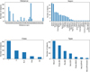 |
Fig. 1 Histograms displaying main properties of objects included in SUCANES. The top panels show the distribution of distances and the star-forming region or the associations the objects belong to. The bottom panels display the evolutionary stage of the objects through the derived ‘class’ parameter (see Sect. 2.1), while the classification of the sources as derived in the different publications is shown in the ‘type’ histogram. |
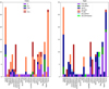 |
Fig. 2 Histogram of SUCANES objects separated by star-forming region. The left histogram displays the number of objects according to their ‘class’, while the right histogram shows the distribution of objects according to their ‘type’, as given in the literature. |
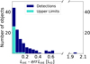 |
Fig. 3 Distribution of Lint-errLint of SUCANES objects. We include detections and upper limits. |
4.2 Envelope masses
From the 174 objects included in SUCANES, we retrieved envelope masses (total mass of gas+dust) for 158 of them. They are represented in Fig. 5. Most of the envelope masses (89 objects) were derived from Herschel/SPIRE flux at 250 µm (objects from Kim et al. 2016). For the 69 left, 35 have masses estimated from 0.85–0.88 mm data, 22 from 1.1–1.3 mm data, and four from 350 µm data. We note that only six objects have masses estimated from interferometric observations (six pre-BDs from Santamaría-Miranda et al. 2021). For eight objects, the masses were estimated through SED or envelope modelling.
From the 121 VeLLOs isolated in Sect. 4.1, 107 have estimated envelope masses. They are highlighted in Fig. 5. As seen, a large fraction of them show Menv < 0.1 M⊙. This is an important parameter since it represents the mass reservoir from which the object will accrete material. Depending on the total mass that is gathered, the object will end up as a brown dwarf or as a star. The total mass accreted by the object can be estimated assuming a core formation efficiency (CFE) in low-mass dense cores. Different works have suggested very different values for this CFE that range from 10–50% (see e.g. Motte et al. 1998; Alves et al. 2007; Bontemps et al. 2010; Palau et al. 2013). Hence, although it is uncertain how much of the envelope mass will finally be accreted by the object, a low value of Menv is required to guarantee that the proto-BD candidate does not reach a stellar mass.
The four objects with Lint< 0.2 L⊙ and Menv > 1 M⊙ are Per-Bolo-58; ChaMMS-1 (see Appendix C); J183014.4-013333, a VeLLO in Aquila identified by Kim et al. (2016); and SM1-A (Kawabe et al. 2018), a proto-BD candidate in the Ophiuchus cloud (objID’s 191, 192, 22, and 325, respectively). While ChaMMS-1 shows properties consistent both with an FHC or a Class 0 object (Maureira et al. 2020), the other three are Class 0 objects. Hence, the four are in a very early stage of their formation; they still have to accrete a significant fraction of their masses and will probably end up as stars and not as BDs.
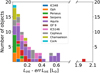 |
Fig. 4 Stacked histogram displaying estimated Lint-errLint for SUCANES objects with revised distances. As seen, several VeLLO candidates (mainly from Aquila) display Lint values above 0.2 L⊙ within the errors. |
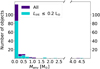 |
Fig. 5 Distribution of envelope masses for all SUCANES objects. We highlight the 107 VeLLOs with Lint ≤ 0.2 L⊙ in cyan. |
4.3 Lbol-Tbol and Lbol,-Lint diagrams
From the 174 objects in SUCANES, we obtained Lbol and Tbol values for 85 objects with well-sampled SEDs. As explained in Sect. 2.3, this means that the objects have data in at least three photometric tables. In practice, we see that most of these objects show data between 3.6 and 850 µm, with an average of ~13 data points to build their SEDs. From these 85 objects, 59 show Lint < 0.2L⊙. We represent this subsample in Fig. 6 (left panel), indicating the number of data points included in their SEDs with colours. As expected, most of the objects in SUCANES show Tbol values below ~650K, which corresponds to an evolutionary stage earlier than or equal to Class I, according to the classification by Chen et al. (1995). There are only three showing slightly higher temperatures: J110955 in Cha I with 700 K, J190418 (in Corona Australis) with 671 K, and J040134.3+411143 in California with 853 K.
The Lbol shows values from 2×10⁻³ to 1.3 L⊙. We have compared these Lbol with the estimated Lint in Fig. 6 (right panel). As expected, Lbol is higher than Lint: this is logical since in embedded objects Lbol is the sum of both the internal and the external luminosity (Lbol = Lint + Lext), where the external luminosity arises from the heating of the circumstellar envelope by the interstellar radiation field. Hence, for a given Lint, the large scatter in Lbol values seen in the figure might reflect a different irradiation of the substellar cores. Figure 6 also shows that it is not simple to estimate the Lint of the objects assuming an approximate percentage of the Lbol, given the high scatter between these two luminosities. To illustrate this, we include a histogram displaying the ratio of the two luminosities (Lbol/Lint) for the displayed sample inside the figure. As seen, around half of the objects show ratios equal to or below 2.5, with the other half displaying ratios above this value (the objects with the highest ratios should be investigated further to undesrtand the origin of these extreme ratios).
5 Scientific application: Future observations of SUCANES objects with ngVLA and SKA
One of the goals of SUCANES is to use the compiled data of pre- and proto-BD candidates to identify the best targets for their future characterisation with forthcoming astronomical facilities. In that respect, two of the most powerful observatories that will be key to characterising large samples of proto-BD candidates are the next generation Very Large Array8 (ngVLA) and the Square Kilometer Array9 (SKA), which will allow us to study radio-jets at the earliest phases of substellar evolution.
If formed as low-mass stars, proto-BDs are expected to show thermal radio jets such as those reported in protostars (e.g. Anglada 1995; Furuya et al. 2003; Anglada et al. 2018). They are also expected to follow well-known correlations reported in young stellar objects that connect stellar and radio-jet properties (e.g. the relation between Lbol and the luminosity at 3.6 cm; e.g. Shirley et al. 2007; Anglada et al. 2018).
Radio jets are studied through centimetre observations: they can either be spatially resolved in a single band, or inferred using the spectral index from two centimeter bands. The first detections of thermal radio jets in a sample of proto-BD candidates were reported by Morata et al. (2015) through Jansky Very Large Array (JVLA) observations at 1.3 cm and 3.6 cm. They observed a sample of 11 proto-BD candidates in the Barnard 213 cloud in Taurus and derived spectral indexes consistent with thermal radio jets in four sources. The detection of these four proto-BD candidates allowed Morata et al. (2015) to extend the Lbol–L3.6 cm relation to very low bolometric luminosities. Using the latest update of that relationship, (Anglada et al. 2018) showed that the proto-BD candidates seem to follow the relation found in more massive YSOs as displayed in Fig. 7 (left panel). However, the figure also reflects the need to increase the number of proto-BD observations at centimetre wavelengths to understand if radio jets are common in these objects and, if so, to extract their main properties.
The intrinsic faintness of proto-BD candidates limits the studies of radio jets. This will change in the near future with the advent of the ngVLA and the SKA observatories. These two facilities will provide superb sensitivity and angular resolution at centimetre wavelengths and, therefore, will be unique facilities to detect and characterise large samples of proto-BD candidates.
As a preparation for future centimetre observations of proto-BD candidates, we selected objects in SUCANES with Lint≤ 0.2 L⊙ and with available Lbol values, and we estimated the expected 3.6cm luminosities assuming they follow the correlation derived by Anglada et al. (2018) for young stellar objects:
 (5)
(5)
The result is shown in Fig. 7 (left panel), where the SUCANES objects occupy the lower left corner of the diagram. Using the derived luminosity at 3.6 cm and the distance to the sources included in SUCANES, we estimated the flux densities at 3.6 cm. We represent them as a function of the bolometric luminosity in Fig. 7 (right panel). As seen, most of the VeLLOs show estimated 3.6 cm flux densities fainter than 200 µJy, with the faintest object displaying a flux of ~16 µJy (Fig. 7, right).
The JVLA 3.6 cm maps presented by Morata et al. (2015) in Barnard 213 reached an average rms of 30 µJy/beam in 4.5–9 minutes of on-source observing time. This sensitivity and the corresponding 5-σ estimation are represented in Fig. 7 with dotted and solid grey lines, respectively. The average synthesised beam was 2.2×1.″8 for uniform weighting and 3.″l × 2.″5 for natural weighting.
We estimated the expected sensitivity levels of ngVLA and SKA at 3.6 cm using the corresponding exposure time calculators (ETC; see below). In both cases, we assumed a target elevation of 45 degrees, a PWV of 6 mm and, for a direct comparison with the JLVA performance, an exposure time (on-source) of six minutes: in the case of ngVLA10, we selected the main array (214 antennas of 18 m) in BAND 2 (3.5–12.3 GHz) considering the full bandwidth of ~8.8 GHz, and native resolution (natural, no taper). We estimated an rms of 0.5 µJy/beam in six minutes of observing time with 25 mas resolution in the continuum. In the case of SKA, we used the SKA-mid sensitivity calculator11 with the AA4 configuration (133 antennas of 15 m), and the Band 5a (4.6–8.5 GHz) using the full bandwidth of 3.8 GHz. We selected natural image weighting and no tapering. The rms obtained after six minutes of exposure time is 1.76 µJy/beam.
The ngVLA and SKA estimations are included in Fig. 7, where the purple and green lines represent the sensitivity (rms and 5-σ) for the two observatories, respectively. As seen, with a relatively modest exposure time investment, ngVLA and SKA-mid will allow us to observe 100% of the sample displayed in Fig. 7 with a signal-to-noise ratio (S/N) >>5 (magenta and green solid lines). Since each observatory will be located in a different terrestrial hemisphere, they will allow us to detect the full sample of young substellar candidates with a high S/N. Moreover, the extrapolation of the data points representing the objects located at similar distances to the left of the plot (i.e. low Lbol values) indicates that SKA and ngVLA will be able to detect radio jets of extremely low-luminosity proto-BDs with Lbol~10−4 L⊙ at 140 pc and Lbol~10−2L⊙ at 600 pc. In any case, and as shown in Sect. 4.3, these Lbol estimations can imply Lint values 2–10 times fainter.
As explained above, the presence of radio jets can be inferred from the spectral index derived using two centimetre bands (see e.g. Anglada et al. 2018). In the case of Morata et al. (2015), they performed observations at 1.3 and 3.6 cm. The expected sensitivity of ngVLA at 1.3 cm (23 GHz), covered by BAND 4 (20.5–34 GHz), is 0.6 µJy/beam after five minutes of exposure time. This is almost 27 times more sensitive than the observations obtained with the JVLA by Morata et al. (2015), with a similar observing time (16 µJy/beam for five minutes on-source). Taking into account that the three proto-BD candidates in Taurus detected at 1.3 cm by the JVLA showed fluxes of 70–80 µJy, ngVLA will definitely help to increase the number of substellar candidates detected at this particular wavelength with a high S/N. The combination of 1.3 cm and 3.6 cm highly sensitive observations will provide spectral indexes for large samples of proto-BD candidates. Finally, we note that although SKA will not initially observe at 1.3 cm, the team will consider a future upgrade covering frequencies up to 24 GHz. Future studies of proto-BD candidates at centimetre wavelengths with ngVLA and SKA will allow us to confirm the true nature of a large sample of very young substellar candidates and characterise their mass-loss processes.
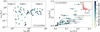 |
Fig. 6 Bolometric luminosities versus the bolometric temperatures and internal luminosities of a subsample of SUCANES objects. Left: Lbol–Tbol diagram with 59 objects from SUCANES with well-sampled SEDs and Lint< 0.2 L⊙ (circles). The dotted vertical lines represent the Tbol values used to classify Class 0/I/II objects according to Chen et al. (1995). Right: Lbol versus Lint for the SUCANES objects with Lint ≤ 0.2 L⊙. The inset histogram represents the distribution of Lbol/Lint ratios for the represented objects. The colours of the circles in the two panels represent the number of data points used to build the SEDs of the objects. |
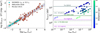 |
Fig. 7 Predicted centimetre luminosities and fluxes versus the bolometric luminosities of SUCANES objects. Left: 3.6 cm luminosities of substellar candidates with Lint < 0.2 L⊙, and with an estimated Lbol in SUCANES (cyan circles). The 3.6 cm luminosities were derived using the correlation (blue dashed line) derived by Anglada et al. (2018) for YSOs (orange squares). We mark the proto-BD candidates studied by Morata et al. (2015) with green squares. Right: estimated 3.6 cm flux densities of the SUCANES objects included in the left panel, using the distances included in our database. The grey lines represent the rms in µJy/beam (dashed) and the 5-σ estimation (solid) from the JVLA observations included in Morata et al. (2015). The magenta and green lines are the expected sensitivities of the ngVLA and SKA-mid facilities, respectively, after six minutes of on-source exposure time. The dashed and solid lines represent the rms (in µJy/beam) and 5-σ estimations, respectively. The data points are colour-coded depending on their distances (see colour bar). The dotted lines represent objects at 140 pc (blue) and 600 pc (light green), revealing that ngVLA will be sensitive to very faint proto-BD candidates with Lbol~104 L⊙ and 102 L⊙ at these distances, respectively. |
6 Conclusions
We built the SUCANES database, which contains a list of objects classified as VeLLOs or substellar candidates at their earliest stages of formation in the literature. The database is a compilation of bibliographic data and has been complemented with photometric data from public archives and catalogues.
We compiled a total of 174 objects and built graphical tools to represent some of their properties. We analysed the contents of the database and reevaluated the classification of some objects after updating their distances and internal luminosities.
SUCANES is designed as a compilation of sources with a bibliographic classification consistent with potential very young substellar candidates. Hence, it could be considered as a starting point to build subsamples of bona fide substellar candidates (as in Palau et al. 2024). We encourage the users to read the bibliographic references provided to understand the properties and classification of any particular source.
The database is public and open to the astrophysical community. Future upgrades of the DB include its implementation with new discoveries and the revision of the nature of the objects based on results from new observations. If possible, we will work on the development of an automatic tool to allow any user to include newly discovered objects.
Data availability
Table B.1 is available in electronic form at the CDS via anonymous ftp to cdsarc.cds.unistra.fr (130.79.128.5) or via https://cdsarc.cds.unistra.fr/viz-bin/cat/J/A+A/695/A13
Acknowledgements
This project has been funded by the European Space Agency-Science Faculty under contract No. 4000129603/19/ES/CM. We acknowledge CAB(CSIC-INTA) and ISDEFE for their support. We are indebted to A. Parras and S. Suarez for their technical support, and to S. Cabañero and C. Valcarcel for the design of the SUCANES webpage and logo of the GUI. NH, DB, MMC, and MMH have been funded by the Spanish grants MCIN/AEI/10.13039/501100011033 PID2019-107061 GB-C6l and PID2023-150468NB-I00. AP acknowledges financial support from the UNAM-PAPIIT IN113119 and IG100223 grants, the Sistema Nacional de Investigadores of CONAHCyT, and from the CONAHCyT project number 86372 of the ‘Ciencia de Frontera 2019’ program, entitled ‘Citlalcóatl: A multiscale study at the new frontier of the formation and early evolution of stars and planetary systems’, Mexico. IdG acknowledges support from grant PID2020-114461GB-IOO, funded by MCIN/AEI/10.13039/501100011033. OM is partially supported by the program Unidad de Excelencia María de Maeztu, awarded to the Institut de Ciències de l’Espai (CEX2020-001058-M). OM is supported by the European Research Council (ERC) under the European Union’s Horizon 2020 research and innovation programme (ERC Starting Grant “IMAGINE” No. 948582, PI: Daniele Viganò). AB acknowledges support from the Deutsche Forschungsgemeinschaft (DFG, German Research Foundation) under Germany’s Excellence Strategy – EXC 2094 – 390783311. K.M. is funded by the European Union (ERC, WANDA, 101039452). Views and opinions expressed are however those of the author(s) only and do not necessarily reflect those of the European Union or the European Research Council Executive Agency. Neither the European Union nor the granting authority can be held responsible for them. Any work using the database are encouraged to include this sentence in their acknowledgments: “This work has made use of the SUCANES database, a joint project funded by ESA Faculty under contract No. 4000129603/19/ES/CM, ISDEFE and CSIC.”
Appendix A SUCANES DB tables
In this appendix we describe the contents of the tables that have been built for SUCANES. Note that the ‘ObjID’ is the unique identifier for each object in SUCANES Data Base, and all the tables are linked by this number. We describe the columns included in each table below:
Main data tables:
Identity table:
Identification number (ObjID)
Name
Sesame name
Position table:
Identification number (ObjID)
RA and RA_hms coordinates (degrees and sexagesimal)
Decl and Decl_dms (degrees and sexagesimal)
Distance (pc)
eDistance: error in distance (pc)
Type (VeLLO, pre-BD, proto-BD, Vello/FHC?, VeLLO/D, proto-BD/D, VeLLO/protostar)
Classification (0, I, 0/I, Flat)
Reference paper(s)
Photometric tables:
Optical and NIR photometry:
Identification number (ObjID)
Flux (Vega magnitude)
Flux error (Vega magnitude)
Filter Identification Number
Reference paper
Spitzer and Herschel photometry:
Identification number (ObjID)
Flux (mJy)
Flux error (mJy)
Filter Identification Number
Reference paper
Sub-mm and cm photometry:
Identification number (ObjID)
Variabilility (only for centimeter table)
Wavelength (micron)
Flux density (mJy)
Flux density error (mJy)
Peak Intensity (mJy/beam)
Peak intensity error (mJy/beam)
Integrated flux (mJy)
Integrated flux error (mJy)
Beam of observations (arcsec)
Position Angle of observations (degrees)
Angular Size of object in x direction (arcsec)
Angular Size of object in y direction (arcsec)
Resolved (0/1)
Position Angle (degrees)
Name of the Instrument
Reference paper
An auxiliary table called Filters describes the filters used for the photometric data: in each of the photometric tables described above (Optical, NIR, Spitzer, Herschel), we include a ‘Filter Identification Number’ after each flux value. This identification is defined as a number that links each photometric filter with the auxiliary table that includes this information:
Filter Identification Number
Filter name
Central wavelength (micron)
FWHM (micron)
Zero point Vega (Jy)
Zero point Vega (erg/cm2/s)
Derived physical parameters tables:
LumTbol table
Identification number (ObjID)
Internal luminosity (L⊙ )
Internal luminosity error (L⊙ )
Bolometric luminosity (L⊙ )
Bolometric temperature (K)
Dust_properties table
Identification number (ObjID)
Wavelength (µm)
Beam of observations (arcsec)
Dust temperature (K)
Opacity (cm2 g−1 )
Dust mass (M⊙)
Total mass (M⊙)
Reference paper
Molecular lines table:
Identification number (ObjID)
CO available data: Yes (1)/ No (0)
C available data : Yes (1)/ No (0)
HCN available data: Yes (1)/ No (0)
HCO+ available data: Yes (1)/No (0)
N2 H+ available data: Yes (1)/ No (0)
CS available data: Yes (1)/ No (0)
CN available data: Yes (1)/ No (0)
CH3OH available data: Yes (1)/ No (0)
SiO available data: Yes (1)/ No (0)
Reference paper(s)
Outflow detected: Yes (1)/No (0)/No information (None)
Molecule used for outflow detection
References for outflow detection
For each molecule, we have included a value of 0 if no data is available, and 1 if there is data, regardless of the detection/non-detection of the object. Note that, for simplicity, we have only included in the table the name of the studied molecule. To look for the particular transition that was observed, the user should check the bibliographic reference(s) provided for each source.
Appendix B Objects included in SUCANES
We summarize in Table B.1 all the objects included in SUCANES. We provide their main properties and the corresponding bibliographic references.
Appendix C Notes on individual sources included in SUCANES
In this appendix we briefly describe the properties of some of the sources included in SUCANES to explain their inclusion in the database:
IRAM04191: This Class 0 object was discovered by André et al. (1999), and classified as a VeLLO by Dunham et al. (2006) after the analysis of Spitzer data. The object was included in the sample analyzed by Kim et al. (2016, 2019) who concluded that is probably a protostar based on its accretion properties, although this classification is highly uncertain, as explained by the authors. Note that there are indirect evidences of this object being a binary system (Lee et al. 2005).
IRAS 04191+1523 B: This object was classified as a proto-BD candidate by Bulger et al. (2014). The target is the secondary component of a binary separated by 6.″1 (Duchêne et al. 2004). Luhman et al. (2010) estimated a spectral type of M6-M8, which impliedthatthe central source is asubstellaroraVery Low Mass object Dang-Duc et al. (2016). The photometry at wavelengths longer than 8µm is contaminated by the primary star emission, which can explain the SUCANES estimated values for Lint and Lbol (0.37 and 0.49 L⊙, respectively). The dynamical mass of the object, derived through ALMA C18O observations, is of 120 MJup after correction from the disc inclination. Hence, the source properties are more consistent with a low-mass protostar and not with a proto-BD.
[GKH94] 41: Luhman et al. (2010) classified the source as ‘Class I?’, but the study of Furlan et al. (2011) concluded that this was a disc-dominated source and probably a more evolved object. However, the analysis of millimeter observations presented by Dang-Duc et al. (2016) revealed the presence of an envelope, confirming that this is a Class I source. They estimate an upper limit to the mass of the central object in the range of 14–97 MJup.
IRAS 04248+2612: This object was classified as a proto-BD by White & Hillenbrand (2004) based on its near-IR and optical properties. The authors reported a spectral type of M5.5 and a central mass of 0.07 M⊙, according to the temperature-mass relation from Siess et al. (2000) evolutionary models at 1 Myr. The target is a triple system (Duchêne et al. 2007), composed by a close binary (separation of 0/16) and a third object at a separation of 4.″55. Bulger et al. (2014) and Mottram et al. (2017) have presented Herschel 70 µm photometry of the unresolved system that results in a Lint of 0.32+0.04 L⊙. The estimated mass of the envelope is 0.25 M⊙ (Motte & André 2001).
IRAS 04158+2805: It was classified as a proto-BD by White & Hillenbrand (2004). However, a work by Luhman (2006) suggested that the object is a low-mass star rather than a brown dwarf. Its evolutionary stage is controversial since it is surrounded by a high inclined disc that can block the stellar light thus mimicking a younger, embedded system (see e.g. the discussion by Ragusa et al. 2021). However, other works show that its properties are more consistent with a Class I source in Taurus (e.g. Furlan et al. 2008). The object has been resolved into a 25 au separation binary, and its total dynamical mass ranges between 0.15–0.45 M⊙. Depending on the mass of each component, it might host at least one substellar object.
IRAS 04489+3042: It was classified as a proto-BD by White & Hillenbrand (2004). However, Luhman (2006) suggested that the object is a low-mass star rather than a brown dwarf.
IRAS 15398-3359: This source was included in SUCANES since Oya et al. (2014) classified it as a substellar object. They provided an upper limit to its mass of <0.09 M⊙ based on the modeling of its rotating infalling envelope. Okoda et al. (2018) estimated a dynamical mass of 0.007 M⊙ based on the fit to a Keplerian motion of the PV diagram of the SO molecule. We estimate a Lint~1.3 L⊙, which is not consistent with a VeLLO. However, Jørgensen et al. (2013) has suggested that such a large Lint could be the result of an accretion burst that took place during the last 100-1000 years.
B1b-N & B1b-S: These two sources are located in the Barnard-1 cloud in Perseus (Hirano et al. 1999). Hirano & Liu (2014), derived Lintvalues consistent with VeLLOs. The new distance of 293+22 pc assumed in SUCANES still provides Lint consistent with that classification (<0.01 L⊙ and 0.05 L⊙ for B1b-N and B1b-S, respectively). Hirano & Liu (2014) concluded that the properties of the two sources are consistent with Class 0 objects less evolved than other Class 0 protostars, with B1-bN displaying properties consistent with a FHC. The study presented by Gerin et al. (2017) using ALMA reached similar conclusions. Hence, B1b-N has been classified as a VeLLO/FHC?, while B1b-S has classified it as ‘VeLLO’. The estimated envelope mass is of 0.56 M⊙ for both objects, using the updated distance of 293 pc (Hirano & Liu 2014).
GF 9-2: Based on its upper limit to the Lint, Palau et al. (2014) classified this object as a VeLLO. We have derived an upper limit to the Lint of < 0.2 L⊙ using the revised distance to GF 9 of 270+10 pc (Clemens et al. 2018). Note that Furuya et al. (2019) have discarded it as a proto-BD candidate based on the estimated envelope infall rate.
Cha MMS-1: This object is embedded in a filament of the Chamaeleon I cloud, and was classified as a possible FHC by Belloche et al. (2011). The Lint derived in SUCANES is 0.02 L⊙. Tsitali et al. (2013) estimated the Lint based on a 3D Radiative magneto-hydrodynamical model to be between 0.13–0.29 L⊙ (for an updated distance of 192 pc). Busch et al. (2020) confirmed the presence of a bipolar outflow in the source through ALMA observations, and argued that its evolutionary stage is more consistent with a Class 0 object than with a FHC. Maureira et al. (2020) presented ALMA observations concluding that although their data could not rule out the object as a FHC, the properties of its CO outflow and SED were in better agreement with the predictions for a young protostar. The mass of the envelope derived from 870 µm single dish data is 5.5 M⊙, considering the total flux associated to the spatially resolved source (Belloche et al. 2011). Given this mass estimation, the object will probably end up as a star. We have included VeLLO/FHC? in its Type field.
L1448-IRS2E: This object was first reported as a VeLLO by Chen et al. (2010). An ALMA study by Maureira et al. (2020) showed neither emission of dense gas (traced by N2H+, and NH2D) at the position of the VeLLO nor detection of any source at the 3.3 mm continuum. They concluded that there is not any core at the position of the target. Instead, they explained the emission reported by Chen et al. (2010) as gas heated by the outflow of the neighboring Class 0 source, L1448 IRS2. Hence, the nature of this object is doubtful.
VeLLOs included in Table 5 from Kim et al. (2019): the 19 targets included in this table are VeLLOs that show outflows. They have been classified either as proto-BD or protostars based on the estimation of the accreted mass and the mass of the envelope. However, this classification should be taken with caution given the associated uncertainties. As explained by the authors, “the estimation of the accreted mass and the envelope mass can be affected by various uncertain parameters, which are mostly unknown, and hence our classification of the sources can be highly uncertain”. One of the objects classified as a possible protostar is IRAM04191 (see above) that we have classified as a proto-BD candidate based on its binarity properties.
J041847.84+274055.3: The infrared object in Taurus (ObjID 163) has been recently identified as a galaxy by Bouy et al. (in prep.) using Euclid data in the visible band. Hence, we have discarded it as a proto-BD candidate, and included a ’D’ in the type column.
References
- Alves, J., Lombardi, M., & Lada, C. J. 2007, A&A, 462, L17 [NASA ADS] [CrossRef] [EDP Sciences] [Google Scholar]
- Alves de Oliveira, C., Moraux, E., Bouvier, J., et al. 2010, A&A, 515, A75 [NASA ADS] [CrossRef] [EDP Sciences] [Google Scholar]
- Andre, P., Ward-Thompson, D., & Barsony, M. 1993, ApJ, 406, 122 [NASA ADS] [CrossRef] [Google Scholar]
- André, P., Motte, F., & Bacmann, A. 1999, ApJ, 513, L57 [Google Scholar]
- André, P., Ward-Thompson, D., & Greaves, J. 2012, Science, 337, 69 [CrossRef] [Google Scholar]
- Anglada, G. 1995, in Revista Mexicana de Astronomía y Astrofísica Conference Series, 1, eds. S. Lizano, & J. M. Torrelles, 67 [Google Scholar]
- Anglada, G., Rodríguez, L. F., & Carrasco-González, C. 2018, A&A Rev., 26, 3 [Google Scholar]
- Barrado y Navascués, D., Stauffer, J. R., Morales-Calderón, M., et al. 2007, ApJ, 664, 481 [CrossRef] [Google Scholar]
- Bate, M. R. 2012, MNRAS, 419, 3115 [NASA ADS] [CrossRef] [Google Scholar]
- Bayo, A., Barrado, D., Huélamo, N., et al. 2012, A&A, 547, A80 [NASA ADS] [CrossRef] [EDP Sciences] [Google Scholar]
- Belloche, A., Schuller, F., Parise, B., et al. 2011, A&A, 527, A145 [NASA ADS] [CrossRef] [EDP Sciences] [Google Scholar]
- Bonnell, I. A., Clark, P., & Bate, M. R. 2008, MNRAS, 389, 1556 [NASA ADS] [CrossRef] [Google Scholar]
- Bontemps, S., Motte, F., Csengeri, T., & Schneider, N. 2010, A&A, 524, A18 [NASA ADS] [CrossRef] [EDP Sciences] [Google Scholar]
- Bourke, T. L., Myers, P. C., Evans, Neal J., I., et al. 2006, ApJ, 649, L37 [NASA ADS] [CrossRef] [Google Scholar]
- Bulger, J., Patience, J., Ward-Duong, K., et al. 2014, A&A, 570, A29 [NASA ADS] [CrossRef] [EDP Sciences] [Google Scholar]
- Busch, L. A., Belloche, A., Cabrit, S., Hennebelle, P., & Commerçon, B. 2020, A&A, 633, A126 [NASA ADS] [CrossRef] [EDP Sciences] [Google Scholar]
- Chen, H., Myers, P. C., Ladd, E. F., & Wood, D. O. S. 1995, ApJ, 445, 377 [NASA ADS] [CrossRef] [Google Scholar]
- Chen, X., Arce, H. G., Zhang, Q., et al. 2010, ApJ, 715, 1344 [NASA ADS] [CrossRef] [Google Scholar]
- Choi, M., Lee, J.-E., & Kang, M. 2014, ApJ, 789, 9 [NASA ADS] [CrossRef] [Google Scholar]
- Clemens, D. P., El-Batal, A. M., Cerny, C., et al. 2018, ApJ, 867, 79 [CrossRef] [Google Scholar]
- Dang-Duc, C., Phan-Bao, N., & Dao-Van, D. T. 2016, A&A, 588, L2 [NASA ADS] [CrossRef] [EDP Sciences] [Google Scholar]
- de Gregorio-Monsalvo, I., Barrado, D., Bouy, H., et al. 2016, A&A, 590, A79 [NASA ADS] [CrossRef] [EDP Sciences] [Google Scholar]
- di Francesco, J., Evans, N. J., I., Caselli, P., et al. 2007, in Protostars and Planets V, eds. B. Reipurth, D. Jewitt, & K. Keil, 17 [Google Scholar]
- Duchêne, G., Bouvier, J., Bontemps, S., André, P., & Motte, F. 2004, A&A, 427, 651 [NASA ADS] [CrossRef] [EDP Sciences] [Google Scholar]
- Duchêne, G., Bontemps, S., Bouvier, J., et al. 2007, A&A, 476, 229 [Google Scholar]
- Dunham, M. M., Evans, II, N. J., Bourke, T. L., et al. 2006, ApJ, 651, 945 [NASA ADS] [CrossRef] [Google Scholar]
- Dunham, M. M., Crapsi, A., Evans, Neal J., I., et al. 2008, ApJS, 179, 249 [NASA ADS] [CrossRef] [Google Scholar]
- Dzib, S. A., Loinard, L., Ortiz-León, G. N., Rodríguez, L. F., & Galli, P. A. B. 2018, ApJ, 867, 151 [Google Scholar]
- Evans, Neal J., I., Dunham, M. M., Jørgensen, J. K., et al. 2009, ApJS, 181, 321 [NASA ADS] [CrossRef] [Google Scholar]
- Furlan, E., McClure, M., Calvet, N., et al. 2008, ApJS, 176, 184 [NASA ADS] [CrossRef] [Google Scholar]
- Furlan, E., Luhman, K. L., Espaillat, C., et al. 2011, ApJS, 195, 3 [Google Scholar]
- Furuya, R. S., Kitamura, Y., Wootten, A., Claussen, M. J., & Kawabe, R. 2003, ApJS, 144, 71 [NASA ADS] [CrossRef] [Google Scholar]
- Furuya, R. S., Kitamura, Y., & Shinnaga, H. 2019, ApJ, 871, 137 [NASA ADS] [CrossRef] [Google Scholar]
- Galli, P. A. B., Loinard, L., Bouy, H., et al. 2019, A&A, 630, A137 [NASA ADS] [CrossRef] [EDP Sciences] [Google Scholar]
- Gerin, M., Pety, J., Commerçon, B., et al. 2017, A&A, 606, A35 [NASA ADS] [CrossRef] [EDP Sciences] [Google Scholar]
- Hennebelle, P., & Chabrier, G. 2008, ApJ, 684, 395 [Google Scholar]
- Hirano, N. 2019, in ALMA2019: Science Results and Cross-Facility Synergies, 90 [Google Scholar]
- Hirano, N., & Liu, F.-c. 2014, ApJ, 789, 50 [NASA ADS] [CrossRef] [Google Scholar]
- Hirano, N., Kamazaki, T., Mikami, H., Ohashi, N., & Umemoto, T. 1999, in Star Formation 1999, ed. T. Nakamoto, 181 [Google Scholar]
- Huélamo, N., de Gregorio-Monsalvo, I., Palau, A., et al. 2017, A&A, 597, A17 [NASA ADS] [CrossRef] [EDP Sciences] [Google Scholar]
- Jørgensen, J. K., Visser, R., Sakai, N., et al. 2013, ApJ, 779, L22 [Google Scholar]
- Kawabe, R., Hara, C., Nakamura, F., et al. 2018, ApJ, 866, 141 [NASA ADS] [CrossRef] [Google Scholar]
- Kim, M.-R., Lee, C. W., Dunham, M. M., et al. 2016, ApJS, 225, 26 [NASA ADS] [CrossRef] [Google Scholar]
- Kim, G., Lee, C. W., Maheswar, G., et al. 2019, ApJS, 240, 18 [NASA ADS] [CrossRef] [Google Scholar]
- Lada, C. J. 1987, in Star Forming Regions, 115, eds. M. Peimbert, & J. Jugaku, 1 [Google Scholar]
- Lada, C. J.. & Wilking, B. A. 1984, ApJ, 287, 610 [NASA ADS] [CrossRef] [Google Scholar]
- Ladd, E. F., Adams, F. C., Casey, S., et al. 1991, ApJ, 366, 203 [NASA ADS] [CrossRef] [Google Scholar]
- Lee, C.-F., Ho, P. T. P., & White, S. M. 2005, ApJ, 619, 948 [NASA ADS] [CrossRef] [Google Scholar]
- Lee, J.-E., Lee, S., Dunham, M. M., et al. 2017, Nat. Astron., 1, 0172 [NASA ADS] [CrossRef] [Google Scholar]
- Luhman, K. L. 2006, ApJ, 645, 676 [NASA ADS] [CrossRef] [Google Scholar]
- Luhman, K. L., Allen, P. R., Espaillat, C., Hartmann, L., & Calvet, N. 2010, ApJS, 186, 111 [Google Scholar]
- Machida, M. N., Inutsuka, S.-i., & Matsumoto, T. 2009, ApJ, 704, L10 [NASA ADS] [CrossRef] [Google Scholar]
- Maureira, M. J., Arce, H. G., Dunham, M. M., et al. 2020, MNRAS, 499, 4394 [NASA ADS] [CrossRef] [Google Scholar]
- Monteiro, H., Dias, W. S., Moitinho, A., et al. 2020, MNRAS, 499, 1874 [NASA ADS] [CrossRef] [Google Scholar]
- Morata, O., Palau, A., González, R. F., et al. 2015, ApJ, 807, 55 [NASA ADS] [CrossRef] [Google Scholar]
- Motte, F., & André, P. 2001, A&A, 365, 440 [NASA ADS] [CrossRef] [EDP Sciences] [Google Scholar]
- Motte, F., Andre, P., & Neri, R. 1998, A&A, 336, 150 [NASA ADS] [Google Scholar]
- Mottram, J. C., van Dishoeck, E. F., Kristensen, L. E., et al. 2017, A&A, 600, A99 [NASA ADS] [CrossRef] [EDP Sciences] [Google Scholar]
- Mužić, K., Scholz, A., Geers, V. C., Jayawardhana, R., & López Martí, B. 2014, ApJ, 785, 159 [Google Scholar]
- Myers, P. C., & Ladd, E. F. 1993, ApJ, 413, L47 [NASA ADS] [CrossRef] [Google Scholar]
- Natta, A., Testi, L., Comerón, F., et al. 2002, A&A, 393, 597 [CrossRef] [EDP Sciences] [Google Scholar]
- Okoda, Y., Oya, Y., Sakai, N., et al. 2018, ApJ, 864, L25 [NASA ADS] [CrossRef] [Google Scholar]
- Ortiz-León, G. N., Loinard, L., Dzib, S. A., et al. 2018a, ApJ, 865, 73 [Google Scholar]
- Ortiz-León, G. N., Loinard, L., Dzib, S. A., et al. 2018b, ApJ, 869, L33 [Google Scholar]
- Ossenkopf, V., & Henning, T. 1994, A&A, 291, 943 [NASA ADS] [Google Scholar]
- Oya, Y., Sakai, N., Sakai, T., et al. 2014, ApJ, 795, 152 [NASA ADS] [CrossRef] [Google Scholar]
- Padoan, P., & Nordlund, Å. 2004, ApJ, 617, 559 [NASA ADS] [CrossRef] [Google Scholar]
- Palau, A., de Gregorio-Monsalvo, I., Morata, Ò., et al. 2012, MNRAS, 424, 2778 [NASA ADS] [CrossRef] [Google Scholar]
- Palau, A., Fuente, A., Girart, J. M., et al. 2013, ApJ, 762, 120 [NASA ADS] [CrossRef] [Google Scholar]
- Palau, A., Zapata, L. A., Rodríguez, L. F., et al. 2014, MNRAS, 444, 833 [NASA ADS] [CrossRef] [Google Scholar]
- Palau, A., Huélamo, N., Barrado, D., Dunham, M. M., & Lee, C. W. 2024, New A Rev. 2024, 99, 101711 [NASA ADS] [Google Scholar]
- Ragusa, E., Fasano, D., Toci, C., et al. 2021, MNRAS, 507, 1157 [NASA ADS] [CrossRef] [Google Scholar]
- Reipurth, B., & Clarke, C. 2001, AJ, 122, 432 [NASA ADS] [CrossRef] [Google Scholar]
- Riaz, B., Vorobyov, E., Harsono, D., et al. 2016, ApJ, 831, 189 [NASA ADS] [CrossRef] [Google Scholar]
- Riaz, B., Thi, W. F., & Caselli, P. 2018, MNRAS, 481, 4662 [Google Scholar]
- Santamaría-Miranda, A., de Gregorio-Monsalvo, I., Plunkett, A. L., et al. 2021, A&A, 646, A10 [NASA ADS] [CrossRef] [EDP Sciences] [Google Scholar]
- Shirley, Y. L., Claussen, M. J., Bourke, T. L., Young, C. H., & Blake, G. A. 2007, ApJ, 667, 329 [NASA ADS] [CrossRef] [Google Scholar]
- Siess, L., Dufour, E., & Forestini, M. 2000, A&A, 358, 593 [Google Scholar]
- Szilágyi, M., Kun, M., & Abraham, P. 2021, MNRAS, 505, 5164 [NASA ADS] [CrossRef] [Google Scholar]
- Tsitali, A. E., Belloche, A., Commerçon, B., & Menten, K. M. 2013, A&A, 557, A98 [NASA ADS] [CrossRef] [EDP Sciences] [Google Scholar]
- Voirin, J., Manara, C. F., & Prusti, T. 2018, A&A, 610, A64 [NASA ADS] [CrossRef] [EDP Sciences] [Google Scholar]
- Wang, J.-W., Lai, S.-P., Clemens, D. P., et al. 2020, ApJ, 888, 13 [NASA ADS] [CrossRef] [Google Scholar]
- Whelan, E. T., Ray, T. P., Bacciotti, F., et al. 2005, Nature, 435, 652 [Google Scholar]
- White, R. J., & Hillenbrand, L. A. 2004, ApJ, 616, 998 [Google Scholar]
- Whitworth, A. P., & Zinnecker, H. 2004, A&A, 427, 299 [NASA ADS] [CrossRef] [EDP Sciences] [Google Scholar]
- Whitworth, A. P., & Stamatellos, D. 2006, A&A, 458, 817 [NASA ADS] [CrossRef] [EDP Sciences] [Google Scholar]
- Young, C. H., Jørgensen, J. K., Shirley, Y. L., et al. 2004, ApJS, 154, 396 [NASA ADS] [CrossRef] [Google Scholar]
- Zucker, C., Speagle, J. S., Schlafly, E. F., et al. 2020, A&A, 633, A51 [NASA ADS] [CrossRef] [EDP Sciences] [Google Scholar]
The internal luminosity is defined as the total luminosity arising from a central object and its disc (including both accretion and photospheric luminosity) and excluding any luminosity arising from the external heating of the surrounding dense core by the interstellar radiation field.
The user manual of the database also includes a link to the Spanish Virtual Observatory filter system for each filter included in this table.
All Tables
All Figures
|
Fig. 1 Histograms displaying main properties of objects included in SUCANES. The top panels show the distribution of distances and the star-forming region or the associations the objects belong to. The bottom panels display the evolutionary stage of the objects through the derived ‘class’ parameter (see Sect. 2.1), while the classification of the sources as derived in the different publications is shown in the ‘type’ histogram. |
| In the text | |
|
Fig. 2 Histogram of SUCANES objects separated by star-forming region. The left histogram displays the number of objects according to their ‘class’, while the right histogram shows the distribution of objects according to their ‘type’, as given in the literature. |
| In the text | |
|
Fig. 3 Distribution of Lint-errLint of SUCANES objects. We include detections and upper limits. |
| In the text | |
|
Fig. 4 Stacked histogram displaying estimated Lint-errLint for SUCANES objects with revised distances. As seen, several VeLLO candidates (mainly from Aquila) display Lint values above 0.2 L⊙ within the errors. |
| In the text | |
|
Fig. 5 Distribution of envelope masses for all SUCANES objects. We highlight the 107 VeLLOs with Lint ≤ 0.2 L⊙ in cyan. |
| In the text | |
|
Fig. 6 Bolometric luminosities versus the bolometric temperatures and internal luminosities of a subsample of SUCANES objects. Left: Lbol–Tbol diagram with 59 objects from SUCANES with well-sampled SEDs and Lint< 0.2 L⊙ (circles). The dotted vertical lines represent the Tbol values used to classify Class 0/I/II objects according to Chen et al. (1995). Right: Lbol versus Lint for the SUCANES objects with Lint ≤ 0.2 L⊙. The inset histogram represents the distribution of Lbol/Lint ratios for the represented objects. The colours of the circles in the two panels represent the number of data points used to build the SEDs of the objects. |
| In the text | |
|
Fig. 7 Predicted centimetre luminosities and fluxes versus the bolometric luminosities of SUCANES objects. Left: 3.6 cm luminosities of substellar candidates with Lint < 0.2 L⊙, and with an estimated Lbol in SUCANES (cyan circles). The 3.6 cm luminosities were derived using the correlation (blue dashed line) derived by Anglada et al. (2018) for YSOs (orange squares). We mark the proto-BD candidates studied by Morata et al. (2015) with green squares. Right: estimated 3.6 cm flux densities of the SUCANES objects included in the left panel, using the distances included in our database. The grey lines represent the rms in µJy/beam (dashed) and the 5-σ estimation (solid) from the JVLA observations included in Morata et al. (2015). The magenta and green lines are the expected sensitivities of the ngVLA and SKA-mid facilities, respectively, after six minutes of on-source exposure time. The dashed and solid lines represent the rms (in µJy/beam) and 5-σ estimations, respectively. The data points are colour-coded depending on their distances (see colour bar). The dotted lines represent objects at 140 pc (blue) and 600 pc (light green), revealing that ngVLA will be sensitive to very faint proto-BD candidates with Lbol~104 L⊙ and 102 L⊙ at these distances, respectively. |
| In the text | |
Current usage metrics show cumulative count of Article Views (full-text article views including HTML views, PDF and ePub downloads, according to the available data) and Abstracts Views on Vision4Press platform.
Data correspond to usage on the plateform after 2015. The current usage metrics is available 48-96 hours after online publication and is updated daily on week days.
Initial download of the metrics may take a while.