| Issue |
A&A
Volume 694, February 2025
|
|
|---|---|---|
| Article Number | A237 | |
| Number of page(s) | 14 | |
| Section | Numerical methods and codes | |
| DOI | https://doi.org/10.1051/0004-6361/202452928 | |
| Published online | 18 February 2025 | |
Fast Bayesian spectral analysis using convolutional neural networks: Applications to GONG Hα solar data
1
Departament de Física, Universitat de les Illes Balears (UIB),
07122
Palma de Mallorca,
Spain
2
Institute of Applied Computing & Community Code (IAC3), UIB,
07122
Palma de Mallorca,
Spain
★ Corresponding author; This email address is being protected from spambots. You need JavaScript enabled to view it.
Received:
8
November
2024
Accepted:
17
January
2025
Abstract
Context. Solar filament oscillations have been observed for many years, but recent advances in telescope capabilities now enable a daily monitoring of these periodic motions. This offers valuable insights into the structure of filaments. A systematic study of filament oscillations over the solar cycle can shed light on the evolution of the prominences. Only manual techniques were used so far to analyze these oscillations.
Aims. This work serves as a proof of concept and demonstrates the effectiveness of convolutional neural networks (CNNs). These networks automatically detect filament oscillations by applying a power-spectrum analysis to Hα data from the GONG telescope network.
Methods. The proposed technique studies periodic fluctuations in every pixel of the Hα data cubes. Using the Lomb-Scargle periodogram, we computed the power spectral density (PSD) of the dataset. The background noise fits a combination of red and white noise well. Using Bayesian statistics and Markov chain Monte Carlo (MCMC) algorithms, we fit the spectra and determined the confidence threshold of a given percentage to search for real oscillations. We built two CNN models to obtain the same results as with the MCMC approach.
Results. We applied the CNN models to some observations reported in the literature to prove its reliability in detecting the same events as the classical methods. A day with events that were not previously reported was studied to determine the model capabilities beyond a controlled dataset that we can check with previous reports.
Conclusions. CNNs prove to be a useful tool for studying solar filament oscillations using spectral techniques. The computing times are significantly reduced for results that are similar enough to the classical methods. This is a relevant step toward the automatic detection of filament oscillations.
Key words: Sun: atmosphere / Sun: chromosphere / Sun: corona / Sun: filaments, prominences / Sun: oscillations
© The Authors 2025
 Open Access article, published by EDP Sciences, under the terms of the Creative Commons Attribution License (https://creativecommons.org/licenses/by/4.0), which permits unrestricted use, distribution, and reproduction in any medium, provided the original work is properly cited.
This article is published in open access under the Subscribe to Open model. This email address is being protected from spambots. You need JavaScript enabled to view it. to support open access publication.
1 Introduction
Solar filaments, also known as prominences when observed off- disk, are dense, cool plasma structures suspended in the hot solar corona by magnetic fields. They appear as dark structures in Hα observations. Despite extensive research, the formation, structure, and disappearance of these filaments are not fully understood. Filaments form within filament channels (FCs), which are large, nonpotential magnetic structures situated above the polarity inversion lines (PILs) in the photosphere. The development of FCs is influenced by motions on the solar surface and subsurface, including differential rotation, meridional flows, and convection (see, e.g., Mackay 2014). Throughout the solar cycle, filaments migrate across different latitudes and form patterns that resemble the sunspot butterfly diagram (McIntosh 1972; Minarovjech et al. 1998; Coffey & Hanchett 1998; Diercke et al. 2024). This migration suggests that filament structures and the large-scale solar magnetic field are related.
Solar prominences exhibit various types of motion, notably oscillations, which have been more frequently observed due to the capabilities of new instruments (Arregui et al. 2018). These oscillations are relevant because they enable prominence seismology to determine the physical parameters of magnetized plasma structures. Oscillations in solar filaments are categorized based on their restoring forces. Transverse oscillations are mainly governed by the Lorentz force (Hyder 1966; Kleczek & Kuperus 1969; Hershaw et al. 2011), while longitudinal oscillations are influenced by gravity along the magnetic field lines and gas pressure gradients (Luna & Karpen 2012; Luna et al. 2012; Zhang et al. 2012; Zhang et al. 2013). Luna et al. (2017) compared field properties derived from filament seismology with the reconstructed magnetic field using the flux-rope insertion method by van Ballegooijen (2004) and found a general agreement. This highlights that oscillation studies can enhance our understanding of filament structures.
Despite the potential insights that systematic studies of filament oscillations offer in the evolution of prominences and their FCs during the solar cycle, most observational research has focused on individual events. One of the few extensive studies was conducted by Bashkirtsev & Mashnich (1993), who reported 38 oscillation events over nearly a solar cycle and noted a sinusoidal latitudinal dependence of the oscillation periods. However, a later study by Luna et al. (2018) did not find a clear relation between oscillation periods and filament latitude. Using Hα data from the GONG network during January–June 2014, Luna et al. provided an extensive sample of 196 events near the solar maximum of cycle 24 and found an average oscillation period of 58 minutes, regardless of amplitude or filament type.
Traditionally, the time-distance technique was used, which involves measuring the intensity along a fixed artificial slit following the motion. This method has been widely applied in the study of oscillations in coronal loops and the detection of solar filament oscillations (see Pant et al. 2016; Zhang et al. 2017; Joshi et al. 2023). However, these methods first require a visual detection of the oscillations, and second, an artificial slit that traces them to construct the time-distance diagram. This means that time-distance diagram methods are not applicable for the automatic detection and parameterization of oscillations in filaments. Luna et al. (2022) introduced a new method by using two-dimensional Hα images and performing spectral (frequency-domain) analysis on the intensity time series of all pixels in the data. This technique allows the automatic detection of oscillations in the solar disk.
Luna et al. (2022) demonstrated that spectral techniques can effectively detect oscillations in solar filaments, and this served as a proof of concept. However, the methods they employed offer room for refinement. Following the approach of Auchère et al. (2016), background noise is typically estimated by fitting the power spectral density (PSD) using a weighted leastsquares method. This fit is weighted by the inverse square of the smoothed PSD, obtained via a five-point boxcar average. Additionally, confidence levels are calculated assuming that the background noise is white noise. The PSD derived from the temporal evolution of pixel intensities is usually a combination of red and white noise. It is challenging to nalyze these PSDs because red noise can mimic or obscure genuine oscillatory signals, which might lead to false detections if it is not properly accounted for. Sophisticated statistical methods are therefore necessary to distinguish true oscillations from noise-induced fluctuations. While some studies have attempted to simplify the analysis by whitening the PSD to mitigate the red-noise component, VanderPlas (2018) emphasized that a more rigorous approach involves following the Bayesian method outlined by Vaughan (2010). This method employ Markov chain Monte Carlo (MCMC) techniques to robustly assess the significance of the detected oscillations.
Although these Bayesian methods offer a statistically robust framework, their computational complexity can be prohibitive for the typically large datasets in solar imaging. In our work, we initially employed the MCMC-based approach, but found it too slow for our research purposes. To overcome this limitation, we decided to use machine learning. In recent years, the field of machine learning has bloomed in popularity in many scientific fields and also in solar physics (see Asensio Ramos et al. 2023), for the benefits it provides in computational efficiency, and because it can process enormous amounts of data. For this reason, we developed a deep-learning model that replicates the predictive capabilities of the MCMC method. This substantially improved the computational efficiency without compromising the accuracy.
The paper is structured as follows. In Sect. 2 the Hα data from the GONG telescope network are described. Section 3 describes the theoretical background for identifying oscillations in red-noise PSD using the methods described in Vaughan (2010). Section 4 presents the deep-learning model, which uses convolutional neural networks (CNNs) as its architecture. Section 5 shows the results for three different observational days, two of which include events that were previously reported in Luna et al. (2018), and one event was not previously reported by other authors. Finally, in Sect. 6, the results are discussed and conclusions are drawn.
2 Data
In Hα images, filaments appear as dark structures against the bright chromospheric background, which makes them particularly useful for studying filament dynamics. This clarity is often lacking in extreme-UV (EUV) data from instruments such as the Atmospheric Imaging Assembly (AIA) from the Solar Dynamics Observatory (SDO) (Lemen et al. 2011), where the more complex and dynamic structures complicate the filament identification and the automated detection of their oscillations.
2.1 NSO-GONG network
The NSO-GONG1 (Hill et al. 1994) telescope network monitors the full disk almost continuously in the Hα wavelength The network consists of telescopes with an identical design and construction that are placed around the globe at the following locations: Learmonth (L), Udaipur (U), El Teide(T), Cerro Tololo (C), Big Bear (B), and Mauna Loa (M). These locations were strategically selected to follow the diurnal motion of the Sun and to ensure full-day coverage. Each telescope in the network captures images during its daytime, with overlapping hours of coverage between consecutive telescopes following the Earth’s rotation. Since the NSO-GONG network is based on the ground, Earth’s atmospheric conditions can influence the observations and should be considered. The Hα GONG data consist of images of 2048×2048 pixels with a nominal spatial resolution of approximately 2 arcsec. Each of the network’s telescopes provides images with a one-minute cadence. The network’s duty cycle is 90%, meaning that due to telescope performance or poor sky quality, the telescope does sometimes not provide the image, and this results in data gaps in the time series.
2.2 Data preparation
We analyze the temporal sequences of GONG Hα images. We grouped the GONG data into full-day bins. Although this choice is arbitrary, it enables the grouping of detections by day. The choice of the length of the time sequences also imposes a limit on the maximum period that can be detected. However, oscillations primarily exhibit periods shorter than a few hours (see, e.g. Arregui et al. 2018; Luna et al. 2018). In the future, longer bins spanning several days will be used to explore oscillations of longer periods, such as those observed by Foullon et al. (2004, 2009) and Efremov et al. (2016).
To construct the Hα time series, it is necessary to combine data from the various telescopes in the GONG network. Each GONG telescope operates for several hours throughout the day, with the possibility of up to four telescopes operating simultaneously. During these overlaps, it becomes necessary to select which telescope’s data to use for constructing the time series. To facilitate this selection process, we employed the following algorithm:
We first segmented the full-day time series into intervals in which data were either absent, available from a single telescope, or overlapped from multiple telescopes. When only one telescope was active, we used its data by default.
When two or more telescopes observed within the same time window, we evaluated the quality of the images produced by each telescope. The telescope providing the highest-quality images was then selected for that segment.
After we constructed the image sequence, we remove limb darkening from the images (Cox 2002). Differential rotation was then compensated for by remapping all images to 12:00 UT using the SunPy2 algorithms. This ensured a consistent intensity across the entire disk and allowed each pixel to correspond to the same area on the solar surface throughout the temporal sequence.
The selection of the appropriate telescope in step 2 was guided by a preference for longer uninterrupted sequences from a single telescope to minimize the frequency of switching between telescopes. Additionally, we considered the average sharpness value of the image sequence as recorded in the FITS metadata to ensure optimal image quality.
After this process, individual images that might have poor quality or atmospheric noise, such as cloud cover, were checked for exclusion. In some cases, only a portion of the solar disk was visible due to issues with the telescope. These images generate rapid intensity variations that result in significant high-frequency noise. To identify these problematic images, quick checks of their circular symmetry relative to the image center were performed. We calculated Pearson’s correlation coefficient between the Hα intensities along the central horizontal and vertical lines, denoted as ρ⊕, as well as along the two main diagonals, denoted as ρ⊗. In high-quality images, both ρ⊕ and ρ⊗ should be similar and close to one, even when dark structures such as filaments are present. To assess the image quality for a day of observations, we proceeded as listed below.
Compute ρ⊕ and ρ⊗ for each image within the corrected temporal sequence.
Calculate the mean values,
 and
and  , and standard deviations,
  and
and  , of these coefficients over the entire temporal sequence.
All images that have either ρ⊕ or ρ⊗ below the threshold defined as
 were considered to have poor quality and were discarded.
Figure 1 shows the effects of the different preprocessing steps we applied. We plot the temporal series of a given pixel on 22 October 2024. In Fig. 1a the full temporal sequence is shown with 1418 candidate images. The limb-darkening and differential rotation were corrected for in these images. Image quality evaluations were applied, and 29 images were removed from the original set. The result is plotted in Fig. 1b. We verified that this technique discarded low-quality images satisfactorily and quickly. Methods are available today for removing clouds from Earth’s atmosphere, based on deep-learning techniques, such as those by Wu et al. (2021) and Chaoui et al. (2023). However, we preferred to remove images containing clouds as they are a relatively small fraction of the full-day data. In addition, it should be ensured that these techniques do not introduce artifacts in the intensity temporal series. We will consider these techniques in future studies.
With the methods described above, we obtained a sequence of data by combining the different telescopes and removing poorquality images. Due to local atmospheric conditions, the Sun’s position above the horizon, slight differences in sensitivities, and so on, the intensities measured by the different network telescopes vary slightly. Figure 1a shows the full-day temporal sequence of the intensity in a given pixel on 22 October 2024 of 1418 images. There is an abrupt drop in intensity in the El Teide data with respect to those from Udaipur and Big Bear. To ensure continuity and avoid intensity jumps during telescope changes, we applied a pixel-wise correction of the intensity differences by computing the median of the last ten intensity values from telescope n and the first ten intensity values from telescope n + 1 each time when a swap occured at time tn. Then, we computed the difference between these two medians and added it to the entire temporal series of telescope n + 1. The values of telescope n + 1were updated, and this operation was repeated for each telescope swap. In this way, a continuous intensity sequence was obtained, as shown in Fig. 1b. The next step was the correction for any outlier pixel intensities that can be present in the corrected temporal data. This was done as follows:
Take a pixel temporal series and compute the moving median with a kernel size of 7.
Subtract this moving median from the original signal, take the absolute value, and compute the standard deviation of the result.
If at any time instant the normalized time series is above four times the obtained standard deviation, set that value in the original data to the median at that instant.
Repeat for all the other pixels.
Finally, the last step is to set all the pixels outside the solar disk equal to zero to remove any signals from regions outside of the disk.
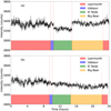 |
Fig. 1 Observation windows from the GONG telescope network for a random pixel during 22 October 2024. The vertical dashed red lines represent the times of a telescope change. (a) Raw time series without any preprocessing. (b) Preprocessed time series. |
3 Spectral analysis: Identifying oscillations
After processing the GONG data, we obtained sequences of images grouped by day through the combination of different telescopes. The obtained time series were normalized and apodized to remove high-frequency noise. This preprocessing resulted in a data cube that was subsequently analyzed as explained in this section. We analyzed the temporal sequences in each of the pixels of the images by constructing a PSD. For each day, 1440 data point are contained in the temporal sequence at most. However, there can be gaps in the data, which results in irregular sampling. For this reason, we used the generalized Lomb-Scargle periodogram (LS-periodogram; Lomb 1976; Scargle 1982; Carbonell & Ballester 1991; Zechmeister & Kürster 2009) to generate the PSD. The term “generalized” indicates that the signal does not need to be zero-averaged, unlike in the original versions of the periodogram (see VanderPlas 2018, for further details). The resulting PSD was normalized following the standard normalization approach outlined in the Astropy documentation3, which resulted in a dimensionless PSD, with values ranging from 0 to 1.
Periodic signals were identified by discerning real oscillations among the noise fluctuations. This was necessary to model the background noise power and determine the confidence level. The background noise power is the PSD of a signal in the absence of real oscillations. The background noise in the GONG data can be modeled as a combination of red and white noise (Luna et al. 2022). For each pixel of the Hα images time series, we considered the background noise power as
 (1)
(1)
where v is the frequency, and A, α, and B are free parameters. The first power-law term models the red noise, and the second constant term is the white noise. The red-noise nature of the PSD adds a layer of complexity to the analysis. Vaughan (2005) proposed a method for analyzing the red-noise section of the spectrum separately from the white-noise part. Using this technique, Gruber et al. (2011) showed that applying a white-noise assumption to data with a power-law PSD drastically overestimates the significance of the detected peaks. Another common way to deal with these data relied on subtracting the background components of the time series (i.e., the moving average). Vaughan (2010) showed that this procedure may lead to misleading results and should be avoided; the entire Fourier spectrum of the signal should always be considered. For these reasons, we used the methods of Bayesian statistics and employed the same techniques as described by Vaughan (2010) and Inglis et al. (2015).
Vaughan (2010) showed the theoretical foundation for parameter estimation in red-noise data using Bayesian statistics and MCMC methods. In general, in this method, given the data D = {D1,…,DN}, a model H, and a set of parameters θ = {θ1,…, θM}, we aim to determine the probability of these parameters given the data and our model, expressed as p(θ|D, H), which is referred to as the posterior distribution. We used Bayes’ theorem, namely
 (2)
(2)
where p(D|θ, H) is the likelihood of the parameters (the probability of the data to occur given that our model and the parameters are true), p(θ|H) is the prior probability (the information about the parameters we have beforehand), and finally, p(D|H) is known as the marginal likelihood (of the data) or the prior predictive distribution that is just a normalization constant.
In this study, the data D consisted of the PSD, where Dj = PSD(vj) in Eq. (2). The model H was given by Eq. (1), and the parameters θ are A, α, and B. The null hypothesis is that our data come from a stochastic process, so that the periodogram was distributed around the background noise (Sj = S (vj)), following a  distribution. With this hypothesis, our likelihood function is
 (3)
(3)
Our prior distributions were uniform probability functions, chosen to reflect our initial lack of specific knowledge about the parameter values, and all values within the specified ranges were considered equally probable. We intentionally selected broad ranges for these priors to avoid imposing restrictive assumptions on the parameter space. The chosen ranges were
 (4)
(4)
These broad prior ranges were selected to encompass the range of likely parameter values while preserving flexibility in our model.
The marginal likelihood p(D|H) is a normalization constant that was computed by integrating the product of the prior probability function and likelihood function over the whole parameter space. This integral is often difficult to compute exactly and may not have an analytical solution. To avoid computing it directly, we used MCMC algorithms to obtain the posterior distribution. After an initial phase called the burn-in period, the Markov chain generated samples of the parameters θ that were distributed according to the Bayesian posterior probability density. In other words, when equilibrium was reached, the distribution of the Markov chain samples mirrored the posterior probability density function (PDF). Consequently, regions in the parameter space that correspond to higher posterior probabilities were sampled more frequently than those with lower probabilities. Therefore, by taking enough samples, we can ensure that we accurately modeled the posterior PDF for the parameters. The posterior PDF contains valuable information: The mode of the parameters θmode provides the best fit to the data with the proposed model. Additionally, with the posterior distributions, the TR test statistic can be computed,
 (5)
(5)
where  is twice the periodogram normalized to the best fit. TR measures the maximum deviation between the observation and the model, and it was used to determine the confidence line of any given percentage, confk%. This line is a threshold for discerning PSD peaks that are due to real oscillations on the time series over noise-generated peaks. We used k% = 95%.
To determine confk%, we began by generating synthetic data based on the posterior distribution of the parameters. This involved creating a large number of parameter vectors θsynth = {θ1,…, θM}synth. By using these vectors in our model, we obtained a set of synthetic best fits Sj (θsynth), which are expected to follow an exponential distribution relative to the real PSD. To simulate synthetic periodogram data, we then multiplied each element of these synthetic best-fit vectors by a random draw from a  distribution. This reflects the expected statistical behavior of the periodogram under the null hypothesis. The resulting synthetic distribution is then
 (6)
(6)
When all the synthetic periodograms were computed, we obtained  .
.
For each frequency, we checked the value of  so that the p value
  was lower than the 1 − k%/100 confidence value we wished to obtain. For example, when we searched for the 95% confidence, the p values should be lower than 0.05.
Finally, the confk% can be obtained from
![Mathematical equation: ${\rm{conf}}_j^{k\% } = R_j^{{\rm{synth}}}\left[ {{p_B} < 1 - k\% /100} \right] \cdot {S_j}\left( {{\theta _{{\rm{mode}}}}} \right)/2.$](/articles/aa/full_html/2025/02/aa52928-24/aa52928-24-eq18.png) (7)
(7)
The confidence line follows the same functional form as in Eq. (1), but is not parallel to the best-fit line and has different parameter values.
We used the Python library PyMC (Abril-Pla et al. 2023) to implement the MCMC algorithm. We used this method to study already reported oscillations in Luna et al. (2018), and the results we obtained agreed with the previously reported results. The results were stored and used for training the deep-learning model presented in the next section. The main problem with the Bayesian technique is the required computing time. The MCMC and confidence line computations take a minimum of 10 seconds for a single pixel. To perform this operation on the entire solar disk using GONG Hα images, it would take approximately 230 days on a single CPU core to process one day of observations. Even with parallelization techniques, this approach is still too slow. To accelerate this computation, we used deep-learning techniques. An important insight is that the k% confidence line can be modeled, as the best-fit line, using Eq. (1). Therefore, we developed a model that can obtain the two sets of parameters that would otherwise result from the MCMC calculation.
 |
Fig. 2 Architecture for the CNN model. The input layers first receive the periodogram, which is then processed by an initial convolutional block (ConvBlock) with kernel sizes of 5 and 8. This is followed by three identical convolutional blocks, each with kernel sizes of 11 and 10. Each ConvBlock concludes with a MaxPooling layer to reduce the dimensionality of the data. All convolutional layers utilize the ReLU activation function. Subsequently, the data is flattened and passed through a compact fully connected neural network with dropout layers. Finally, the network predicts the three target parameters, which are normalized within the range of 0 to 1. |
4 Convolutional neural network
CNNs have demonstrated their effectiveness in numerous scientific fields, including solar physics (Asensio Ramos et al. 2023). We present a simple CNN model capable of predicting the set of parameters for the best fit and a k% confidence line of an MCMC algorithm for a given input PSD. The tools we developed and present here are a proof of concept of the capabilities of CNNs for the analysis of solar data. They also demonstrate of how powerful these tools proved to be for our research purposes. We used a server equipped with an NVIDIA RTX A5000 GPU to train our deep-learning model, which was capable of estimating the best-fit and confidence line parameters for each pixel on the whole solar disk in approximately 5 minutes after it was trained.
4.1 Architecture
The architecture we employed is illustrated in Fig. 2. The model expects as input a periodogram and outputs a vector with the values of A, α, and B for either the best-fit or the confidence line.
The network began with an input layer that took the normalized LS-periodogram, followed by four convolutional blocks (ConvBlock). Each ConvBlock consisted of two 1D convolutional layers with 64 kernels and ReLU activation, followed by a max-pooling layer with a filter size of 2. The first ConvBlock used kernel sizes of 5 and 8, and the subsequent blocks used kernel sizes of 11 and 10. Following the convolutional blocks, a small fully connected network with dense layers containing 1024, 512, and 256 units was employed, each using ReLU activation. To reduce overfitting, dropout layers with a 20% drop probability were included after each dense layer. Finally, the output consisted of a dense layer with three units, each corresponding to one of the parameters to be predicted (A, α, and B). This layer used sigmoid activation because the output data were normalized to values between 0 and 1.
We used the Adam optimizer (Kingma 2014) and a mean- squared error to train the model. To improve the performance, a learning-rate decay schedule was applied, where the learning rate remained constant for the first ten epochs, and after every fifth epoch, the learning rate decreased by a factor of 0.7. To prevent overfitting with this schedule, we also incorporated an early stop at which we monitored the validation loss. The training was performed for a maximum of 100 epochs. We found the most suitable batch size to be 32.
4.2 Training and validation data
We modeled the PSD best fit and its k% confidence line for a given input periodogram. We employed two datasets to train the neural network. The first dataset consisted of a real data analysis using MCMC (Sect. 3), although its size was relatively small due to the slow nature of the calculations involved, rendering it insufficient for an effective training. To overcome this limitation, a second dataset was generated synthetically, which allowed us to significantly increase the amount of available information for training purposes. The synthetic data were constructed using real data as a reference. Specifically, we used the posterior distributions derived from the MCMC method and parameterized them. Random noise was then introduced to these parameters to introduce slight variations. From these modified posterior distributions, we derived the best-fit parameters and confidence intervals using the methods described in Sect. 3. The corresponding periodograms were constructed from the bestfit parameters and the null hypothesis based on the Bayesian approach (see also Vaughan 2010 for details in the appendices). The best-fit line was multiplied by random values sampled from an exponential distribution to mimic the same statistical behavior as the real data. We generated a total of 2 × 10⁶ synthetic periodograms, each associated with a best fit and confidence interval parameter set. The data were divided using a standard 80–20 split for training and validation. Input features were scaled to a range of 0 to 1 by default, and outputs were normalized using a logarithmic transformation followed by min-max scaling to further constrain values between 0 and 1.
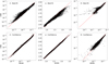 |
Fig. 3 Scatter plots of the expected parameters (MCMC) in the x-axis and the predicted parameters (CNN) in the y-axis for all the periodograms from the testing dataset. The top row shows the best-fit predictions, and the bottom row shows the 95% confidence prediction. |
4.3 Model testing
To assess the reliability and performance of the CNN model, we compared its results with those obtained from observational data. From GONG data, we created a testing dataset of 105 periodograms selected randomly from different observation days, and the best fit and confidence curves were computed using the MCMC techniques.
Figure 3 shows a comparison of the predicted distributions of expected parameters (MCMC) in the x-axis and predicted parameters (CNN) in the y-axis. The top row shows the bestfit model, and the bottom row shows the 95% confidence model. In an ideal case, all predictions should lie on top of the dashed diagonal red line, so that for any given input, both methods (MCMC and CNN) should predict exactly the same values. The narrower the distribution around the dashed red line, the better the model performance. The distributions for the best-fit model are wider than the 95% confidence model, indicating a poorer performance. Both models struggle with the predictions of the B parameter. This parameter shows the most outliers and wide distributions. Using the predicted parameters, we computed the lines given by Eq. (1).
Figure 4 shows the relative errors between the CNN and MCMC model predictions for the best-fit (horizontal axis) and confidence lines (vertical axis). The mean relative error for the best-fit line is approximately 8%, and for the confidence interval, it is 4%. These values indicate that the errors for the best-fit line are higher than those for the 95% confidence line errors on average, but they remain within acceptable limits.
Figure 5 shows three examples of periodograms, together with their corresponding best-fit and confidence curves. These examples were selected from the test dataset and are marked with red dots in Fig. 4. Fig. 5a shows case (1) with a relative error of 2% in the best fit and confidence line. Both sets of curves almost overlap in the entire frequency domain we considered. The second example in Fig. 5b displays a greater discrepancy between the CNN and MCMC results. For the best-fit and confidence curves, the relative errors are 6% and 5%, respectively. Despite a slight separation between the curves, they are nearly identical across most of the frequency range. Finally, Fig. 5c shows case (3), where the errors exceed 10% on average. This is the worst case shown in Fig. 5 with an error of 11% on the best-fit line and 10% on the confidence line. Both sets of curves exhibit the largest discrepancies, with a greater deviation observed in the best-fit case. A detailed inspection reveals that the MCMC curve deviates and the model result performs better. In contrast, the confidence line shows more consistent results for both methods. Fig. 4 shows that cases like (3), where the errors are high, are rare. Specifically, for our testing dataset, we found that only 2% of the periodograms have an error of more than 10% on average.
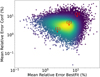 |
Fig. 4 2D histogram representing the percent relative errors found in the testing dataset. The horizontal axis shows the best-fit errors, and the vertical axis shows the confidence line error. The colors represent the density of points. Yellow indicates the highest-density zones, and purple shows the lowest-density zones. The mean values of the distributions are μconfidence = 4% and μbest − fit = 8%. The red dots indicate samples from the different regions of the distribution that are visualized in the next figure. |
5 Results: Study of different events
In this section, we apply the neural network model to three different days of GONG data. The first two days include events that were reported in the Luna et al. (2018) catalog (hereafter referred to as “the catalog”). In this way, we evaluate the validity of the model. The third case shows new oscillations, on which we prove the ability of the model to detect new events.
5.1 1 January 2014
Figure 6 shows the oscillation analysis of the full disk for 1 January 2014. To construct these figures, the ratio of the PSD to the 95% confidence curve was calculated. We only considered cases with a positive detection, that is, when PSD/conf95% ≥ 1. Additionally, the frequency range was divided into bins of 0.055 mHz, spanning from 0.136 to 0.461 mHz. The panels display the maximum ratio of the PSD and the confidence level within each frequency bin. This ratio is overplotted on the Hα images (which have an increased contrast for better visualization of the filaments). This allowed us to determine whether the oscillations were associated with the filaments. In the catalog, two different events are reported (events 1 and 2) in the same filament, placed almost at the center of the disk (x, y) ≈ (−18, −76) arcsecs. This is shown in Fig. 6b with a black box. The first event was reported to have a period of 75.2 ± 1.0 minutes, and the second event had a period of 71.2 ± 2.8 minutes.
Figure 6a shows the ratio in the first bin, between 87– 122 minutes. Numerous smaller dispersed regions are present, many of which are not on filaments. Panel 6b shows considerable power over the three filaments marked with boxes between the periods of 68 to 87 minutes. The filament enclosed with a black box corresponds to events 1 and 2 with the period in this frequency range. This shows that the findings of the CNN model agree with the results of the catalog. Additionally, there is also power around another two filaments that are marked with red boxes. These oscillations were not reported in the catalog.
Similarly to panel 6a, small areas are detected and are scattered around the disk. Figure 6c shows the power distribution between 55 and 68 minutes. This panel shows that the central filament also has power in this period range. This indicates that the oscillations associated with events 1 and 2 of the catalog are distributed in two frequency bins. As we detail below, the reason is that the PSD has a Gaussian distribution with at least these two bins. Additionally, some power is visible in the other two filaments shown in 6b, along with a fourth filament that is enclosed in a red box in the south-central region of the disk, centered at approximately (x, y) = (400, −400) arcsecs. For the northernmost highlighted filament, the PSD is distributed around the filament structure and displays multiple frequencies that exceed the confidence threshold. The most significant contributions come from the two frequency bins that correspond to period ranges of 68–87 minutes and 55–68 minutes. In the following panels, Fig. 6d to Fig. 6e, some power also appears over the filaments. However, across the disk, it is seen in the form of small regions. Similarly, in Fig. 6f, numerous small regions are scattered across the disk. Notably, there is significant power in the western solar plage, which is attributed to the activity in this active region (AR). Small filaments also exhibit PSD values above the confidence threshold, marking the detection of additional oscillations in various frequency bins. While a detailed analysis of these smaller filaments is beyond the scope of this paper, they represent an important dataset for future statistical research. To reduce the number of figures, we omit panels similar to Fig. 6, which correspond to periods shorter than 36 minutes. In these panels, numerous small regions of relatively low power appear to be scattered across the disk.
Fig. 7a shows the Hα intensity in a pixel within the region marked with a black box in Fig. 6b. The best fit and confidence lines constructed with our neural network model are also plotted in Fig. 7b. This figure is similar to the results presented in Fig. 5 by Luna et al. (2022). It is important to note that in their figure, both lines (the confidence line and the fit) are parallel. In contrast, our case clearly shows nonparallel lines because we aplied a more advanced technique (Sect. 3).
In Fig. 7a periodic fluctuations are clearly present from approximately 5:00 to 16:00 UT. These periodic fluctuations are associated with the passage of the filament over the pixel that produces periodic occultations of the chromosphere. In the PSD shown in Fig. 7b, the most significant peak is centered at 73 minutes, with a value of approximately three times the confidence level. This is well above the threshold. This detection agrees with the results found in the catalog. This peak falls into two different frequency bins, showing power in both panels Figs. 6b and 6c. A secondary peak is centered at 64 minutes, with values that are almost twice as high than the confidence threshold. In addition, other peaks in different frequencies are also above the confidence threshold, as in a peak around 30 minutes, and multiple peaks presented below 10 minutes. However, these frequencies are more localized in space, as shown in Figs. 6d to 6f, where small areas appear over the filament. This indicates that this type of filament oscillation is multiperiodic. This might be associated either with the existence of overtones and/or with oscillations of different parts of the filament with different periodicities along the line of sight.
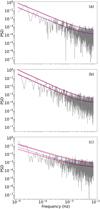 |
Fig. 5 Periodograms with the predicted best-fit and 95% confidence curves from the test dataset, highlighted as red dots (1), (2), and (3) in Fig. 4. Panel a: Region (1) with the smaller errors. Panel b: Region (2) with average errors. Panel c: Region (3) with the highest errors. |
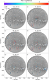 |
Fig. 6 Ratio of the PSD over the predicted confidence line from the CNN model for 1 January 2014 over the background Hα intensity map (the Hα maps have an artificially increased contrast for clearer visualization of the dark structures). The predictions were binned in frequency with an increment of 0.055 mHz. We show the approximate period ranges associated with each frequency bin. The black boxes represent events reported in Luna et al. (2018) within the respective period range. The red boxes represent newly detected events that are thought to be related to filament oscillations that are further discussed in the text. |
5.2 13 February 2014
Figure A.1 shows the oscillatory analyses performed for 13 February 2014. The catalog reports two events on this day, events 62 and 63. Event 62 was reported for a filament centered around (x, y) = (600, 239) arcsecs with a period of oscillation of 47.6 ± 0.6 minutes. Event 63 was reported in a large filament southwest of the disk at approximately (x, y) = (708, −382) arcsecs, with a period of 103.3 ± 0.4 minutes. The panels of Figure A.1 represent the same frequency bins as we considered previously. Similarly to the previous case, many detection zones appear in the different bins, scattered around the disk. Fig. A.1a shows considerable PSD around the filament southwest of the disk, highlighted with a black box. This corresponds to event 63 from the catalog. Similar results are shown in Fig. A.1b. Panel A.1c, like in all the other considered bins, has a scattered PSD through the disk, but a remarkable detection is shown in the active region placed at (x, y) = (300, −100) arcsecs. This is highlighted with a red box. Fig. A.1d shows regions in the filament in which event 63 was reported. Additionally, another filament north of this region is clearly detected. Both filaments are highlighted with a black box. This detection, absent in the previous bins, corresponds to event 62 from the catalog. Like in the previous case studied, the detection peak of this event falls between two of the bins. This means that there are detection zones in panel e in similar zones as in panel d for the two events reported in the catalog. Finally, Figs. A.1e and A.1f again shows the concentration of the PSD in the active region.
Figure 8a shows the temporal evolution of a pixel for which the ratio PSD/conf95% was highest for event 63. Fig. 8b shows the corresponding periodogram with the CNN-predicted best-fit and 95% confidence curves. The main peak is centered around 100 minutes, but a secondary peak lies at ~50 minutes and more between 40 to 30 minutes. The position of the main peak agrees with Luna et al. (2022) Fig. 6c, but in their figure, these secondary peaks are not visible. The presence of these peaks needs to be treated with caution. Luna et al. (2022) reported a secondary period associated with the filament crossing its equilibrium position, with a period that is half of the primary oscillation period. The PSD at this period is concentrated over the filament. This does not imply that a zone detected at half the period of the stronger signal always is an artifact of this type; however, some of these detections should be examined with caution. In future statistical studies, these cases will be addressed using alternative techniques to avoid reporting events that result from this limitation of the method.
Finally, Fig. 9 shows the average temporal evolution of the AR with the associated periodogram. As shown in panel 9a, the active region exhibits a repetitive sequence of intensity peaks associated with C- and M-class flares according to the Heliophysics Events Knowledgebase (HEK; Hurlburt et al. 2012) database. In panel 9b, the positions of the three main peaks are aligned with the visual results from Figs. A.1c, A.1e, and A.1f. The primary peak is centered at 39 minutes, followed by another peak at 47 minutes, and the final peak at 66 minutes. These results demonstrate that our techniques can detect other periodic events within solar chromosphere observations and are not limited to filament oscillations alone. This reveals the effectiveness of this machine-learning approach.
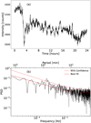 |
Fig. 7 Time series and spectral analysis results from a pixel inside the black box from Fig. 6b. Panel a Hα intensity as a function of time during the 24 hours of 1 January 2024. Panel b Corresponding PSD and the predicted best fit (solid red line) and 95% confidence line (dashed red line). |
5.3 22 October 2024
Finally, we analyzed the data for 22 October 2024. This day has not previously been studied and was selected because a large number of filaments appear. As in the previous cases, Fig. B.1 shows the PSD in the different bins obtained from the CNN predictions.
In Figs. B.1a–B.1f, the PSD is predominantly scattered across the solar disk. Notably, there are specific regions where the PSD exhibits concentrations near filaments; these areas are highlighted with black boxes in the corresponding frequency bins. These concentrations suggest localized oscillatory phenomena associated with filament structures. Specifically, Figs. B.1a and B.1b show an event at the small filament located at approximately (x, y) ≈ (−320, 80) arcsec with periods exceeding 70 minutes. The subsequent panels highlight three additional filaments that demonstrate PSD concentrations in various frequency bins, indicating multiple periodicities. The easternmost filament, situated at (x, y) ≈ (−400, −200) arcsec, shows an event triggered by a C-class flare (according to the HEK database) at around 12:10:00 UT that emanates from a nearby active region. This flare induces movement at the eastern end of the filament, resulting in oscillations of the entire structure. The complexity of these oscillations is evident; multiple periodicities are detected in different regions of the filament, as depicted in Figs. B.1c to B.1f. These observations highlight the intricate coupling between flares and filament dynamics. Another significant filament oscillation is observed at coordinates (x, y) ≈ (100, −400) arcsec, as shown in Figs. B.1d and B.1e. This event corresponds to a periodic movement of the filament without an apparent external trigger, as no immediate cause is evident from the visual inspection of its temporal evolution. A dedicated study is required to understand what triggered this oscillation. Finally, the westernmost event involves the filament located at (x, y) ≈ (680, 10) arcsec. The periodicities associated with this filament are display c, d, and f. This filament oscillation ed in Fig. B.1 panelswas initiated by a C-class flare event that occurred around 15:20:00 UT from a small active region situated to the south. The flare induced motion in the filament, causing it to oscillate with different periods. Shortly after the initial flare, a subsequent C-class flare occurred and caused it to erupt and disappear from the Hα data. Our CNN model effectively detects and analyzes solar filament oscillations, as demonstrated by the successful identification of oscillatory events on 22 October 2024. By automating the detection and spectral analysis processes, the model enhances the efficiency and comprehensiveness of studying filament dynamics. This contributes to a deeper understanding of the physical mechanisms involved.
6 Summary and conclusions
We have investigated the detection of oscillations in images using machine-learning techniques. Following the approach of Luna et al. (2022), we applied a spectral technique that analyzed periodic intensity fluctuations in each pixel of GONG Hα data. First, we generated data cubes by stacking the images from a day collected by the various GONG telescopes. The images to be used were automatically selected from all the telescopes in the network, and low-quality images were discarded, the intensity of the images from different telescopes was regularized, and differential rotation was compensated for. This resulted in a data cube that covered an entire day. The temporal cadence was one minute, which meant that ideally, there would be 1440 images per day. However, not always are images available, or they may have been eliminated during our selection process. This can result in gaps in the time sequence. For each of the pixels in the data cube, the PSD was calculated using the Lomb-Scargle periodogram. As usual in these spectral techniques, we considered a detection to occur when a PSD peak exceeded a certain threshold above the background noise. The background noise is well modeled by a combination of red and white noise.
The background noise signal was determined by fitting the PSD to a model, which was a combination of red and white noise in our case. Additionally, several techniques were available to establish the confidence line. However, the most appropriate technique in the presence of red noise in addition to white noise apparently relies on Bayesian statistics and MCMC techniques (Vaughan 2010), as recommended by VanderPlas (2018, see their Sect. 7.4.2.4). While these methods are powerful for analyzing red-noise periodograms, they proved to be too slow for our research purposes. To address this, we developed a CNN with training data obtained from the MCMC method. The CNN predicted the same results as the MCMC method, but with a drastically shorter computing time. This advancement enhances the efficiency of detecting filament oscillations in large datasets and facilitates more comprehensive studies of these solar phenomena. We performed a thorough error analysis of our deep-learning model and obtained error margins of 5% on average on the predicted curves. This is acceptable for our research objectives. The model capabilities were validated by comparing its results with spectral analyses previously reported by Luna et al. (2022) and with classical methods from Luna et al. (2018). The CNN demonstrated a high accuracy in predicting the oscillation periods, which confirmed its reliability for this application. Furthermore, we applied our CNN to a new set of observations from a day that was not previously studied. Using our model, we identified various types of filament oscillation events. This showed that the CNN can detect and classify oscillations in unseen data. This not only highlights the generalization capabilities of the model, but also contributes new findings to the study of solar filament dynamics.
In conclusion, we proved the effectiveness of machinelearning techniques by application of a CNN to the detection and analysis of oscillations in GONG Hα images. This technique yielded results that are comparable to those of Bayesian methods while significantly reducing the computation time by several tens of thousand times. This will enable us to analyze vast amounts of information to detect oscillations in the GONG data.
We analyzed oscillations in the Hα data without distinguishing whether they belonged to filaments. We showed that periodic flares and many regions outside filaments can be found. For a massive study, segmentation techniques will be used to determine the location of oscillations relative to filaments. This will be the subject of a follow-up study. Although the technique presented in the current work has been implemented for GONG data, it could also be applied to other datasets, such as the EUV images from the SDO. This would enable the detection of oscillations not only in filaments, but also in coronal loops and other structures. In future work, we will apply this technique to SDO data.
Data availability
The code is publicly available in the following repository: https://github.com/GuillemCastello/PeriodogramCNN.
Acknowledgements
This publication is part of the I+D+i project PID2023- 147708NB-I00 funded by MICIU/AEI/10.13039/501100011033/ and by FEDER, EU. It has been also part of the R+D+i project PID2020-112791GB-I00, financed by MCIN/AEI/10.13039/501100011033. M. Luna acknowledges support through the Ramón y Cajal fellowship RYC2018-026129I from the Spanish Ministry of Science and Innovation, the Spanish National Research Agency (Agencia Estatal de Investigación), the European Social Fund through Operational Program FSE 2014 of Employment, Education and Training and the Universitat de les Illes Balears. The authors also thank Prof Ramón Oliver for his helpful comments and suggestions.
Appendix A Results from 13 February 2014
Appendix B Results from 22 October 2024
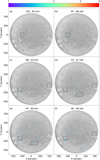 |
Fig. B.1 Same as Fig. 6 but for 22 October 2024. Black boxes highlight regions of interest identified in the analysis and discussed in the text. |
References
- Abril-Pla, O., Andreani, V., Carroll, C., et al. 2023, Peer J Comput. Sci., 9 [Google Scholar]
- Arregui, I., Oliver, R., & Ballester, J. L. 2018, Liv. Rev. Sol. Phys., 15, 3 [Google Scholar]
- Asensio Ramos, A., Cheung, M. C. M., Chifu, I., & Gafeira, R. 2023, Liv. Rev. Sol. Phys., 20, 4 [NASA ADS] [CrossRef] [Google Scholar]
- Auchère, F., Froment, C., Bocchialini, K., Buchlin, E., & Solomon, J. 2016, ApJ, 825, 110 [Google Scholar]
- Bashkirtsev, V. S., & Mashnich, G. P. 1993, A&A, 279, 610 [NASA ADS] [Google Scholar]
- Carbonell, M., & Ballester, J. L. 1991, A&A, 249, 295 [NASA ADS] [Google Scholar]
- Chaoui, A., Morgan, J. P., Paiement, A., & Aboudarham, J. 2023, Removing cloud shadows from ground-based solar imagery, iSSN: 2693-5015 [Google Scholar]
- Coffey, H. E., & Hanchett, C. D. 1998, in IAU Colloq. 167: New Perspectives on Solar Prominences, eds. D. F. Webb, B. Schmieder, & D. M. Rust, Astronomical Society of the Pacific Conference Series, 150, 488 [NASA ADS] [Google Scholar]
- Cox, A. N., ed. 2002, Allen’s Astrophysical Quantities (New York, NY: Springer) [CrossRef] [Google Scholar]
- Diercke, A., Jarolim, R., Kuckein, C., et al. 2024, A&A, 686, A213 [NASA ADS] [CrossRef] [EDP Sciences] [Google Scholar]
- Efremov, V. I., Parfinenko, L. D., & Solov’ev, A. A. 2016, Sol. Phys., 291, 3357 [NASA ADS] [CrossRef] [Google Scholar]
- Foullon, C., Verwichte, E., & Nakariakov, V. M. 2004, A&A, 427, L5 [NASA ADS] [CrossRef] [EDP Sciences] [Google Scholar]
- Foullon, C., Verwichte, E., & Nakariakov, V. M. 2009, ApJ, 700, 1658 [NASA ADS] [CrossRef] [Google Scholar]
- Gruber, D., Lachowicz, P., Bissaldi, E., et al. 2011, A&A, 533, A61 [NASA ADS] [CrossRef] [EDP Sciences] [Google Scholar]
- Hershaw, J., Foullon, C., Nakariakov, V. M., & Verwichte, E. 2011, A&A, 531, A53 [NASA ADS] [CrossRef] [EDP Sciences] [Google Scholar]
- Hill, F., Fischer, G., Forgach, S., et al. 1994, Sol. Phys., 152, 351 [NASA ADS] [CrossRef] [Google Scholar]
- Hurlburt, N., Cheung, M., Schrijver, C., et al. 2012, Sol. Phys., 275, 67 [Google Scholar]
- Hyder, C. L. 1966, ZAp, 63, 78 [NASA ADS] [Google Scholar]
- Inglis, A. R., Ireland, J., & Dominique, M. 2015, ApJ, 798, 108 [Google Scholar]
- Joshi, R., Luna, M., Schmieder, B., Moreno-Insertis, F., & Chandra, R. 2023, A&A, 672, A15 [Google Scholar]
- Kingma, D. P. 2014, arXiv preprint [arXiv:1412.6980] [Google Scholar]
- Kleczek, J., & Kuperus, M. 1969, Sol. Phys., 6, 72 [NASA ADS] [CrossRef] [Google Scholar]
- Lemen, J. R., Title, A. M., Akin, D. J., et al. 2011, Sol. Phys., 275, 17 [Google Scholar]
- Lomb, N. R. 1976, Astrophys. Space Sci., 39, 447 [Google Scholar]
- Luna, M., & Karpen, J. 2012, ApJ, 750, L1 [NASA ADS] [CrossRef] [Google Scholar]
- Luna, M., Díaz, A. J., & Karpen, J. 2012, ApJ, 757, 98 [Google Scholar]
- Luna, M., Su, Y., Schmieder, B., Chandra, R., & Kucera, T. A. 2017, ApJ, 850, 143 [NASA ADS] [CrossRef] [Google Scholar]
- Luna, M., Karpen, J., Ballester, J. L., et al. 2018, ApJS, 236, 35 [NASA ADS] [CrossRef] [Google Scholar]
- Luna, M., Mestre, J. R. M., & Auchère, F. 2022, A&A, 666, A195 [NASA ADS] [CrossRef] [EDP Sciences] [Google Scholar]
- Mackay, D. H. 2014, in Solar Prominences (Springer), 355 [Google Scholar]
- McIntosh, P. S. 1972, Rev. Geophys. Space Phys., 10, 837 [CrossRef] [Google Scholar]
- Minarovjech, M., Rybanský, M., & Rušin, V. 1998, Sol. Phys., 177, 357 [NASA ADS] [CrossRef] [Google Scholar]
- Pant, V., Mazumder, R., Yuan, D., et al. 2016, Sol. Phys., 291, 3303 [NASA ADS] [CrossRef] [Google Scholar]
- Scargle, J. D. 1982, ApJ, 263, 835 [Google Scholar]
- van Ballegooijen, A. A. 2004, ApJ, 612, 519 [NASA ADS] [CrossRef] [Google Scholar]
- VanderPlas, J. T. 2018, ApJS, 236, 16 [Google Scholar]
- Vaughan, S. 2005, A&A, 431, 391 [NASA ADS] [CrossRef] [EDP Sciences] [Google Scholar]
- Vaughan, S. 2010, MNRAS, 402, 307 [NASA ADS] [CrossRef] [Google Scholar]
- Wu, X., Song, W., Zhang, X., et al. 2021, Comput. Mater. Continua, 71, 3497 [Google Scholar]
- Zechmeister, M., & Kürster, M. 2009, A&A, 496, 577 [CrossRef] [EDP Sciences] [Google Scholar]
- Zhang, Q. M., Chen, P. F., Xia, C., & Keppens, R. 2012, A&A, 542, A52 [NASA ADS] [CrossRef] [EDP Sciences] [Google Scholar]
- Zhang, Q. M., Chen, P. F., Xia, C., Keppens, R., & Ji, H. S. 2013, A&A, 554, 124 [Google Scholar]
- Zhang, Q. M., Li, D., & Ning, Z. J. 2017, ApJ, 851, 47 [NASA ADS] [CrossRef] [Google Scholar]
All Figures
|
Fig. 1 Observation windows from the GONG telescope network for a random pixel during 22 October 2024. The vertical dashed red lines represent the times of a telescope change. (a) Raw time series without any preprocessing. (b) Preprocessed time series. |
| In the text | |
|
Fig. 2 Architecture for the CNN model. The input layers first receive the periodogram, which is then processed by an initial convolutional block (ConvBlock) with kernel sizes of 5 and 8. This is followed by three identical convolutional blocks, each with kernel sizes of 11 and 10. Each ConvBlock concludes with a MaxPooling layer to reduce the dimensionality of the data. All convolutional layers utilize the ReLU activation function. Subsequently, the data is flattened and passed through a compact fully connected neural network with dropout layers. Finally, the network predicts the three target parameters, which are normalized within the range of 0 to 1. |
| In the text | |
|
Fig. 3 Scatter plots of the expected parameters (MCMC) in the x-axis and the predicted parameters (CNN) in the y-axis for all the periodograms from the testing dataset. The top row shows the best-fit predictions, and the bottom row shows the 95% confidence prediction. |
| In the text | |
|
Fig. 4 2D histogram representing the percent relative errors found in the testing dataset. The horizontal axis shows the best-fit errors, and the vertical axis shows the confidence line error. The colors represent the density of points. Yellow indicates the highest-density zones, and purple shows the lowest-density zones. The mean values of the distributions are μconfidence = 4% and μbest − fit = 8%. The red dots indicate samples from the different regions of the distribution that are visualized in the next figure. |
| In the text | |
|
Fig. 5 Periodograms with the predicted best-fit and 95% confidence curves from the test dataset, highlighted as red dots (1), (2), and (3) in Fig. 4. Panel a: Region (1) with the smaller errors. Panel b: Region (2) with average errors. Panel c: Region (3) with the highest errors. |
| In the text | |
|
Fig. 6 Ratio of the PSD over the predicted confidence line from the CNN model for 1 January 2014 over the background Hα intensity map (the Hα maps have an artificially increased contrast for clearer visualization of the dark structures). The predictions were binned in frequency with an increment of 0.055 mHz. We show the approximate period ranges associated with each frequency bin. The black boxes represent events reported in Luna et al. (2018) within the respective period range. The red boxes represent newly detected events that are thought to be related to filament oscillations that are further discussed in the text. |
| In the text | |
|
Fig. 7 Time series and spectral analysis results from a pixel inside the black box from Fig. 6b. Panel a Hα intensity as a function of time during the 24 hours of 1 January 2024. Panel b Corresponding PSD and the predicted best fit (solid red line) and 95% confidence line (dashed red line). |
| In the text | |
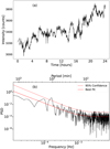 |
Fig. 8 Same as Fig. 7, but for a pixel from the black box highlighting event 63 from the catalog. |
| In the text | |
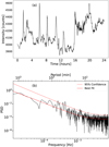 |
Fig. 9 Same as Fig. 7, but for the average of the AR at (x, y) = (300, −100) from 13 February 2014. |
| In the text | |
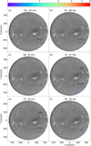 |
Fig. A.1 Same as Fig. 6 but for 13 February 2014. |
| In the text | |
|
Fig. B.1 Same as Fig. 6 but for 22 October 2024. Black boxes highlight regions of interest identified in the analysis and discussed in the text. |
| In the text | |
Current usage metrics show cumulative count of Article Views (full-text article views including HTML views, PDF and ePub downloads, according to the available data) and Abstracts Views on Vision4Press platform.
Data correspond to usage on the plateform after 2015. The current usage metrics is available 48-96 hours after online publication and is updated daily on week days.
Initial download of the metrics may take a while.