| Issue |
A&A
Volume 694, February 2025
|
|
|---|---|---|
| Article Number | A111 | |
| Number of page(s) | 11 | |
| Section | The Sun and the Heliosphere | |
| DOI | https://doi.org/10.1051/0004-6361/202452278 | |
| Published online | 07 February 2025 | |
Connecting energetic electrons at the Sun and in the heliosphere through X-ray and radio diagnostics
1
LESIA, Observatoire de Paris, PSL Research University, CNRS, Sorbonne Université, Université Paris Cité, 5 place Jules Janssen, 92195 Meudon, France
2
Goddard Planetary Heliophysics Institute, University of Maryland, Baltimore County, Baltimore, MD 21250, USA
3
Heliospheric Physics Laboratory, Heliophysics Division, NASA Goddard Space Flight Center, Greenbelt, MD 20771, USA
4
Radboud Radio Lab, Department of Astrophysics/IMAPP-Radboud University, NL-6500 GL Nijmegen, The Netherlands
⋆ Corresponding author; This email address is being protected from spambots. You need JavaScript enabled to view it.
Received:
17
September
2024
Accepted:
12
December
2024
Abstract
Context. Solar flares release huge amounts of energy, a considerable part of which is channeled into particle acceleration in the lower corona. Hard X-ray (HXR) emissions are used to diagnose the accelerated electrons that bombard the chromosphere, while type III radio bursts result from energetic electron beams propagating through the corona and into interplanetary space. The Solar Orbiter mission, launched in 2020, aims to link solar flare remote observations with heliospheric events, thus producing useful observations for our understanding of particle acceleration and propagation from the Sun to the heliosphere.
Aims. While both hard X-Ray and radio emissions result from flare-accelerated electrons, their relationship is not straightforward. By comparing the evolution of the X-ray emitting sites and the timing of type III bursts, our aim is to determine the conditions for associations between X-ray flares and interplanetary (IP) type III bursts.
Methods. We analyzed 15 interplanetary type III bursts that are associated with HXR bursts in the first available period for simultaneous X-ray/radio observations of type III bursts from Solar Orbiter (using the RPW and STIX instruments). X-ray imaging was performed around the onset of the type III bursts, complemented by EUI 174 Å images to assess the magnetic configuration of the corona.
Results. All 15 X-ray flares originated from the same active region on the west limb as observed by Solar Orbiter. In each of the events, a change in X-ray source morphology occurred shortly (< 6 minutes) before the onset of type III radio bursts, indicating a change in the electron acceleration region preceding the radio emission. Considering the delays observed between the two emissions, these findings describe complex scenarios with multiple reconnection episodes, some of which may allow accelerated electrons to escape into IP space when open magnetic field lines are involved (interchange reconnection). In some cases, X-ray source elongations toward open field lines in the UV were observed, reinforcing this idea.
Key words: Sun: corona / Sun: flares / Sun: radio radiation / Sun: X-rays / gamma rays
© The Authors 2025
 Open Access article, published by EDP Sciences, under the terms of the Creative Commons Attribution License (https://creativecommons.org/licenses/by/4.0), which permits unrestricted use, distribution, and reproduction in any medium, provided the original work is properly cited.
This article is published in open access under the Subscribe to Open model. This email address is being protected from spambots. You need JavaScript enabled to view it. to support open access publication.
1. Introduction
The Sun efficiently accelerates particles during solar flares. In particular, electrons carry an important fraction of the energy released from non-potential coronal magnetic fields through magnetic reconnection in the low corona (see Emslie et al. 2012). Flare-accelerated electrons are detected both directly in interplanetary space once they escape the Sun, and indirectly through X-ray/γ-ray and radio emissions originating from the solar surface and the high corona, respectively. Accelerated electron beams interact with the solar atmosphere and the denser chromosphere, radiating hard X-rays (HXRs) via bremsstralung. HXRs provide the most direct diagnostics of flare-accelerated electrons and of the hottest flare plasma. Nonthermal HXR sources are usually found at chromospheric footpoints of flare loops. However, fainter coronal sources have also been detected (e.g., Sui et al. 2005; Battaglia & Benz 2006; Krucker et al. 2007). When the energetic electrons reach open magnetic field lines in the corona, they can produce radio emission in the corona as they propagate into interplanetary space. During their propagation in the background plasma, electron beams generate Langmuir waves and produce coherent radio emission via the plasma emission mechanism (type III bursts). The radio emission is produced at the plasma frequency (fundamental emission) or twice the plasma frequency (harmonic emission). As the plasma frequency depends on the square root of the local plasma electron density, type III radio bursts can be observed over a wide frequency range, from high frequencies in the corona (GHz) to low frequencies (kHz) as the beam propagates away from the Sun. Type III bursts produced in the low corona (from the GHz range to 10 MHz) can be observed from the ground and are sometimes called coronal type III bursts. On the other hand, type III bursts reaching frequencies below 14 MHz are called interplanetary (IP) bursts. They cannot be measured from the ground, but only by instruments on board spacecrafts (see review by Reid 2020).
Many studies relating the observations of coronal type III radio bursts and HXR emissions have been performed since the first observations of their temporal association (e.g., Kane 1972, 1981). Several statistical studies have been performed on the correlation of hard X-ray and radio type III bursts (Hamilton et al. 1990), but also on the association of hard X-ray emissions and any kind of coherent radio emission (type IIIs, but also pulsations, continua, and narrowband spikes) in the decimetric range (100 MHz–4 GHz) (Benz et al. 2005). In this last study it was found that nearly all flares with a GOES class above C5 are associated with coherent radio emissions in the 100 MHz–4 GHz range. Classic meter wave type III bursts were found in 33% of all X-ray flares, but they were the only radio emission in only 4% of the events. No coherent emission in the decimetric/metric band was found for 17% of the HXR flares, and all these flares either had radio emission at lower frequencies or were limb events (Benz et al. 2007).
More recently, the statistical study done by Reid & Vilmer (2017) has shown that while not all coronal type III bursts have an interplanetary counterpart, coronal type III bursts associated with X-ray flares that are bright at high energies (25–50 keV) are more systematically associated with interplanetary type III bursts. In James & Vilmer (2023) a weak correlation is observed between the number of high-energy electrons (deduced from the nonthermal X-ray radiation) in the flare and the peak flux of the coronal type III burst observed from ground-based observatories. However, while some correlations exist, it has been found that not all strong hard X-ray bursts are associated with type III producing electron beams. The magnetic topology of the flaring active region (i.e., with mostly closed magnetic loops and no access to open magnetic field lines) also plays a major role in the potential association of HXR flares and type III bursts. In more recent studies, Krupar et al. (2024) and Kruparova et al. (2024) also show relevant correlations between the radio flux of type III bursts and the intensity of the associated GOES flares. They also suggest that the relationship may be influenced by other factors such as the position of the flares and the observational conditions.
As recalled in the previous paragraph, the conditions that determine the escape of flare-accelerated electrons from the flare site into interplanetary space have been extensively studied. The magnetic configuration of the active region plays a key role in determining whether flare accelerated particles remain confined or can propagate higher in the solar corona and in the association rate between HXR emissions and radio bursts. The association between hard X-ray and type III emissions can thus be further investigated by examining the spatial correspondence between X-ray and radio sources close to the Sun and higher in the corona (see Vilmer et al. 2002). In some cases, observations of this kind support that type III generating electrons are produced by the same acceleration mechanism as HXR emitting electrons since a close link is found between the evolution of X-ray and radio sources on a timescale of a few seconds (Vilmer et al. 2002). However, in other cases the link between HXR emissions and radio decimetric/metric emissions is more complicated. The radio emissions can originate from several locations, one very close to the X-ray emitting site, another farther away from the active region, and more linked to the radio burst at lower frequencies (e.g., Vilmer et al. 2003). These observations are consistent with the cartoon presented in Benz et al. (2005), in which the electrons responsible for type III emissions at low frequencies are produced in a secondary reconnection site at higher altitudes than the main site responsible for X-rays. Such a scenario for particle acceleration in flares involving two reconnection sites, one involving open field lines (allowing electron beams producing type III bursts to escape) and with reconnection driven by a rising loop system, is reminiscent of the emerging flux model proposed in Heyvaerts et al. (1977). The most discussed flare topology involving reconnection of emerging loops with open magnetic field lines is interchange reconnection (e.g., Crooker & Webb 2006; Baker et al. 2009). In such a topology, precipitating electrons are expected to produce three footpoints in the chromosphere: two at the footpoints of the flare loop and a third at the footpoint of the open field line (see the cartoon in Fig. 7 adapted from Glesener et al. 2012).
Previous studies relating escaping and radio emitting electrons with hard X-ray emitting electrons (e.g., Krucker et al. 2011, Glesener et al. 2012, and more recently Battaglia et al. 2023 for a microflare) support the interchange reconnection geometry for the production of the upward-moving electrons. The appearance of a jet of hot plasma, detected in the extreme ultraviolet (EUV), is additional support for the scenario of interchange reconnection.
Understanding the mechanisms behind the acceleration, propagation, and escape of flare-accelerated electrons into the heliosphere is an active field in solar and heliospheric physics, and a key scientific objective of the Solar Orbiter mission (Müller et al. 2020). Launched in early 2020, Solar Orbiter combines in situ and remote-sensing observations, and is thus very appropriate to study the link between solar flare observations and emissions produced by energetic particles propagating in the heliosphere. Previous statistical studies were achieved with data that were not recorded by instruments on the same platform, which considerably reduces the size of the sample (for observations obtained over more than ten years, the data samples for the statistical studies previously discussed contain only a few hundred simultaneous observations of hard X-ray flares and type III bursts). The present study illustrates what can be done with the new instruments on Solar Orbiter to further explore the conditions that allow flare-accelerated electrons to escape into interplanetary space. This paper presents a detailed analysis of the first period of combined X-ray observations of flares and radio observations of type III bursts, during a five-day interval between November 17 and 21, 2020, recorded during the second commissioning phase of the Spectrometer Telescope for Imaging X-rays (STIX) instrument. Many more combined observations from STIX and the Radio and Plasma Waves Instrument (RPW) are now available. Using these few examples, we thus intend to demonstrate the capabilities of the instruments on Solar Orbiter and how they will bring new results on the link between flare-accelerated electrons and escaping electrons.
2. Instruments and data
The Solar Orbiter commissioning phase started briefly after its launch in February 2020 and finished in November 2020. This study is based on observations in the second commissioning phase of STIX, specifically in the five days from 17 November 00:00 UT to 21 November 23:59 UT, when the STIX and RPW instruments provided the first simultaneous observations of X-ray flares and type III radio bursts from the same spacecraft. At this time Solar Orbiter was at an angle of 122° with respect to the Earth–Sun line, and at a distance of 0.92 AU from the Sun, thus making it difficult to perform combined remote observations with other observatories. A representation of the spacecraft’s position relative to the Earth is displayed in Figure 1.
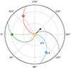 |
Fig. 1. Relative locations of the Sun (orange), Earth (green), and Solar Orbiter (blue) on November 18, 2020. The distance of Solar Orbiter to the Sun is 0.92 AU. The position of the active region mentioned in Sect. 5 (later classified as AR 12785) is marked with a black arrow. The positions of Stereo A is also shown (red). This diagram was prepared with the Solar-MACH tool by Gieseler et al. (2023). |
2.1. STIX Data
The STIX instrument was designed to measure solar X-rays in the energy range of 4–150 keV; it provides information on the flare plasma’s hottest temperatures (≳10 MK) on the spectrum, and the energy spectrum of flare-accelerated nonthermal electrons. The instrument uses a bi-grid system to modulate the incoming signal, allowing the reconstruction of images of the solar X-ray source (Krucker et al. 2020). The level 1 (L1) pixel data files contain information on the counts detected in each pixel and is used to estimate the visibilities, a fundamental component in the process of image reconstruction. Conversely, L1 spectrogram files provide the accumulation of counts per energy channel over all the detectors, which is the most useful quantity for spectroscopy. Unlike the limited availability of L1 pixel data, L1 spectrogram files offer a continuous time series representation spanning extended periods. While L1 pixel data is limited to selected flares, L1 spectrogram files offer broader coverage for temporal analysis and spectroscopy. The STIX team supplies L1 background count rate files, aiding background subtraction for flare analysis. For this work, we used mainly the pixel data to produce images made with the subcollimators calibrated to the date (grids 3–10), corresponding to a finest angular resolution of 14.6″. While STIX can achieve a maximum time cadence of 0.1 seconds, for the data used in this work the highest cadence corresponds to 0.5 s for spectrograms and 2 s for pixel data.
Working with data from this particular time period has disadvantages that must be considered when interpreting the data. First, the STIX Aspect System (SAS), which measures the pointing of STIX relative to the Sun (with a precision of ±4″ in optimal capacity), does not give a reliable solution when the distance between the Sun and Solar Orbiter is larger than 0.75 AU. Furthermore, it does not respond beyond 0.82 AU, as described by Warmuth et al. (2020). In order to create flare images during the selected period, from a distance of ∼0.92 AU, the software automatically uses the spacecraft aspect plus the average offset of STIX determined from events observed early in the mission. This information is provided as L2 auxiliary data files by the STIX team. This limitation reduces the accuracy in determining the absolute location of the imaged X-ray sources; it can lead to offsets going from a few arcseconds up to around one arcminute. Given that there are no sudden maneuvers of Solar Orbiter during the observation period, the positions of the X-ray sources relative to each other and the observations on their shape can be trusted. Another problem present at this period comes from the energy calibration. During the late 2020 checkout window, the electronic setup of the detectors for energy calibration was slightly different compared to when calibration measurements were taken to define the energy lookup table (ELUT), resulting in an average energy offset of around 1.6 keV for each detector-pixel. As fitting this offset pixel-wise is not currently possible, a proposed solution that was used in this work is to subtract the average energy offset from each energy bin uniformly.
2.2. RPW Data
The RPW can measure in situ electric and magnetic fields, plasma wave spectra, and polarization properties. The instrument measures the spectral density of plasma waves in the radio spectral range from very low frequencies (∼0 Hz) up to 16.4 MHz. The Low Frequency Receiver and Thermal Noise Receiver (LFR and TNR respectively) measure frequencies below 1024 kHz, while the High Frequency Receiver (HFR) measures from 0.4 MHz to 16.4 MHz (Maksimovic et al. 2020; Vecchio et al. 2021). For the L3 data files of both receivers used in this study the time resolution varies across the five-day observation period. In the case of the TNR, the length of the time bins is predominantly around 12 s, with values ranging from 3 to 84 s. Conversely, the HFR has a time resolution of 53 seconds throughout most of the observation period, with values between 7 and 175 s.
Some frequency channels in both receivers exhibit contamination from spacecraft-related interferences, as noted in Maksimovic et al. (2021). For instance, as shown in Figure 2, continuous noise contamination is evident within the 2–3 MHz range and around 5 MHz in the HFR data. Additionally, periodic radio bursts caused by the satellite’s battery charging process appear around 394 kHz, typically lasting about an hour. To mitigate these effects, we used uncontaminated channels where possible and interpolated the signal for affected frequencies. Despite these corrective measures, residual contamination remains detectable in the spectra. However, this contamination does not significantly impact the overall accuracy of our type III burst analysis.
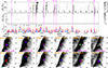 |
Fig. 2. Overview of RPW/STIX observations for a 40-hour time interval from November 18 at 00:00 UT to November 19 at 18:00 UT. (Top) From top to bottom, the panels correspond to RPW-TNR spectrograms (100–425 kHz), RPW-HFR spectrograms (from 425 kHz up to 8 MHz), and STIX count rate light curves at low energy (6–10 keV, red) and high energy (10–16 keV, blue; 16–26 keV, green) ranges. The vertical lines indicate the time of type III onsets in our sample (the associated flare ID number is shown above the radio spectrograms). (Bottom) For six selected flares within this interval, X-ray contours in two energy bands are overlaid on EUV images provided by the EUI in the 174 Å band. Contours are shown for the same energy ranges as the light curves on the STIX count rate plot; the color-coding per energy range is the same as in the top panels. |
2.3. EUI Data
The Extreme Ultraviolet Imager (EUI) on board Solar Orbiter observes the Sun in the extreme ultraviolet wavelength range. It consists of the Full Sun Imager (FSI) and two high-resolution imagers (HRIs), which are optimized to image in Lyman-α and EUV (174 Å, 304 Å) to provide observations from the chromosphere up to corona (Rochus et al. 2020). During the selected observation period in the commissioning phase only FSI was taking images of the Sun, generally once every hour in the 174 Å band. These images are our only way of observing the context of the flares detected by STIX during the whole observation period as this wavelength is sensible to temperatures ≳1 MK, allowing the solar corona and its dynamic processes to be observed.
The FSI has a spatial resolution of 10″ and allows the imaging of plasma structures in the solar atmosphere with exposures of a few seconds. Given the large distance from the Sun during the five-day observation period, the imaging capabilities of the FSI were limited as the Sun is seen with an angular radius of around 1039″ (∼0.29°).
2.4. Data repositories
The L1 pixel and spectrogram data files for STIX, and the L2 auxiliary files with ancillary data used in this study were retrieved from the Solar Orbiter Archive (SOAR) website1 and the Solar Orbiter STIX Data Center2. The L2 EUI FSI images were also retrieved from SOAR. The L3 RPW spectrograms (HFR and TNR) were provided by the RPW team (European Space Agency & Maksimovic 2024) and the daily summary plots are available on the LESIA RPW website3.
3. Overview on the observation period
Despite the challenges stemming from studying events from such an early period in the mission, this first period available for combined STIX/RPW measurements have provided useful observations (see Table 1) from both instruments. According to the flare catalog available in the STIX Data Center, 232 solar flares were captured by STIX, while a total of 32 type III radio bursts were manually identified in the RPW spectrograms. The type III identification was done in the HFR range as this frequency range is where the earliest signal of the type IIIs is seen, and shows the smallest delay between the type III start and the injection at the Sun of the energetic electrons. Only type III bursts with peak flux measurements of at least two orders of magnitude above the background level were considered.
Summary of the X-ray flares and interplanetary type III bursts (IT3) observed by STIX and RPW, respectively, between 17 and 21 November 2021.
Examining the entire five-day period reaffirms the complex connection between X-ray flares and the occurrence of associated IP type III bursts. The correspondence between these two types of emission is not strictly one-to-one, as already pointed out in previous studies. For illustration, a 30-hour subset of combined observations between 18 and 19 November is shown in Figure 2. The strongest X-ray flare detected (with a GOES classification of M2.8) took place on November 18 at around 06:00 UT. It has a relevant count rate in energy ranges extending up to 80 keV, and lacks a corresponding type III counterpart. In radio, the most pronounced IP type III burst event was detected on the same day, occurring at approximately 13:10 UT (event 8; see Fig. 2). Unlike the previous example, this one appears to be linked to a comparatively modest HXR flare (GOES B-class, discussed in detail in Fig. 5) with no discernible counts exceeding 16 keV. Furthermore, the IP type III burst in the latter case does not correspond to the main peak in HXR emission within the 10–16 keV range, but rather has a very good time correlation with a smaller HXR burst that occurred approximately 30 minutes prior.
Table 1 reports the daily occurrence of flares and type IIIs per day, as well as the association rate between these emissions. Significant variations are observed throughout the five days; for instance, the majority of the flares occurred between November 17 and 18 (33% and 25%, respectively). The number of flares per day declines as the five-day period passes, reaching its minimum on November 20 (∼9%). This is also evident in Figure 2, where the X-ray activity is considerably reduced after November 19 06:00 UT. In the radio domain, the most active day was November 18, where almost one-half of the type IIIs were detected (41%). The other days have between four and six type IIIs per day, less than one-half of the events observed on November 18. Furthermore, we assessed the association between X-ray flares and type IIIs by examining the ratios of association; the ratio RR quantifies the fraction of detected type IIIs that could be associated with HXR peaks, and the ratio Rx addresses the association of HXR flares with type IIIs (see Table 1). While 66% of all type IIIs are associated with HXR bursts, there is a discernible downward trend in RR on a daily basis, declining from over 65% in the initial three days to 25% and below after November 20.
In contrast, only 9% of HXR flares had HXR peaks temporally correlated with an interplanetary type III burst (quantified by RX). It is worth noting that the ratio of association RX appeared to peak on November 18 (15%) and 19 (9%), whereas November 17, the day with the highest flare frequency, had a ratio of RX of 7%. This is discussed further in Section 6. In the following sections, the study focuses on a subset of radio bursts where a temporal association between with an HXR peak and a type III burst could be clearly established. Further details on the selection criteria are described in the next section.
4. Methodology
The rest of the paper focuses on IP type III bursts temporally associated with HXR peaks. Given this association, we assumed that the electron beams producing the IP type III bursts and the HXR emissions originate from a common acceleration site. When possible, we used images from the EUI in the 174 Å wavelength to provide the context of the HXR images. Each step of the performed analysis and its motivation is explained in more detail in the following subsections.
4.1. Sample selection and timing
Table 1 shows that 21 IP type III bursts can be temporally associated with a HXR flare. In order to determine the timing of the two emissions as accurately as possible, Python software was developed to produce combined plots of STIX counts rates and of RPW dynamic spectra. The plots were used to track the HXR count rate in time periods close to the onsets of the radio bursts and to select the X-ray observations associated with each type III. Further selection criteria are given below:
-
Availability of L1 STIX pixel data. To image the X-ray sources with good accuracy, only flares with a significant count rate are considered. This discards the faintest flares in the 4–10 keV range in order to have a reliable image reconstruction (peak count rates below 20 counts s−1).
-
Onset time and starting frequency of type III bursts. In order to establish a better temporal association of type IIIs with the HXR peaks in the flare, the radio bursts seen closer to the acceleration source in the Sun should be measured. Thus, we considered only type III bursts for which onset time and starting frequency can be measured above 0.5 MHz, implying that they are detected by RPW-HFR.
This reduces the sample to 15 flares. Some combined plots of the selected flares are displayed in Figures 3, 4, 5, and 6. While hard X-ray spectroscopy may provide information on the energy distribution of the flare nonthermal electrons, only a few selected events have enough counts at high energies to characterize the nonthermal part of the X-ray spectrum. To maintain a reasonable sample size, we do not conduct a spectroscopic study in this paper.
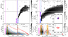 |
Fig. 3. Examples of two events with a good association between type III radio bursts and X-ray emissions observed on 19 and 21 November 2020 (Flares 12 and 15, respectively). The plots from top to bottom correspond to RPW-TNR spectrograms (40–425 kHz), RPW-HFR spectrograms (from 425 kHz up to 8 MHz), and STIX count rate spectrograms with overlayed light curves of the 6–10, 10–16, and 16–26 keV energy ranges (red, blue, and green, respectively). X-ray images are produced for two time intervals (highlighted in orange) of each example. The images of flare 12 are shown in Figure 2. |
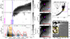 |
Fig. 4. Observations of X-ray and radio emissions of a solar flare on November 17 ∼ 01:25 UT as seen by STIX and RPW (flare 1 in Table A.1). (left) The plots from top to bottom correspond to RPW/TNR (40–425 kHz) and RPW/HFR (from 425 kHz to 8 MHz) spectrograms and STIX count rate spectrogram with light curves of different energy ranges overlayed (4–10, 10–16 and 16–23 keV in red, blue and green respectively). The X-ray flare onset time, the IP type III burst onset time and the time of the associated X-ray peak are marked with vertical lines in magenta, blue, and purple. (center) The sequence of images 1, 2 and 3 correspond to the X-ray imaging of the selected time intervals. For each of them, a EUI/FSI image in the 174 Å band (dark is enhanced emission) is shown with the hard X-ray emission contours overlaid. The contour levels are at 30%, 50%, 70%, and 90%. The integration time (in seconds) used for doing each STIX image is indicated. (right) On the bottom, a zoom of the HXR imaging of interval 3 is overlayed on a running EUI difference image (areas with enhanced emission in the second image relative to the first one appear brighter). In the top image (EUV image of the active region), the frames used for the running difference image (purple frame) and the STIX image of interval 3 (yellow frame) are highlighted. |
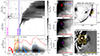 |
Fig. 5. Observations of X-ray and radio emissions of a solar flare on November 18 ∼ 13:00 UT as seen by STIX and RPW (flare 8 in Table A.1). For more details on the different plots, see the caption in Fig. 4. |
As seen in Figures 3, 4, 5, and 6, the onset of IP type III bursts is not necessarily associated with the first HXR peak of the flare (see, e.g., Flare 12 in Fig. 3), but it may be associated with later peaks. For each event of our sample, we made the association of the IP type III burst with the nearest peak of X-ray emissions observed at high energies. The time delay between the type III onset time and the starting time of the X-ray flare Do as well as the time delay between the associated HXR peak and the onset time of the radio burst Dp are measured for each event and indicated in Table A.1. The onset time of X-ray flares is determined by identifying the moment when the count rate in the thermal range exceeds the 3σ threshold above background fluctuations.
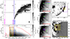 |
Fig. 6. Observations of X-ray and radio emissions of a solar flare on November 18 ∼ 22:25 UT as seen by STIX and RPW (flare 11 in Table A.1). For more details on the different plots, see the caption in Fig. 4. |
4.2. Imaging hard X-ray sources
Once the onset times of the IP type III bursts were determined, the X-ray flares were imaged in energy ranges from 4 to 26 keV, covering time intervals around the associated HXR peaks and focusing on periods shortly before and during the emission of the radio bursts. The images were produced in three different energy ranges: a low energy range from 4 to 10 keV (available for all flares) and two higher energy bands, from 10 to 16 and 16 to 26 keV for the flares with significant counts in these energy channels. All images were produced using the Expectation Maximization (EM) algorithm (Benvenuto et al. 2013) adapted for STIX and available in the STIX-GSW IDL software package4 for SolarSoftware (SSW). The integration time for imaging is set around 50 seconds and chosen according to the X-ray count rate. The time intervals are minimized to increase temporal resolution, but long enough to have robust statistical reliability for the image reconstruction.
Images in ultraviolet from the EUI/FSI are available for some of the X-ray flares that can be imaged. For these flares, the reconstructed X-ray images are overlayed on the nearest available UV image. Furthermore, when UV images are available both before and after the flare, typically with about a one-hour interval between them, a running difference image is made to highlight the changes in the magnetic configuration in the corona around the flare time. However, difference images are not considered for UV images with a larger time gap between them.
5. Observations and data analysis
5.1. General observations
The 15 flares imaged in our sample are listed in Table A.1. Images of the 15 X-ray flares show that all of the flares occurred in the same active region on the right limb of the Sun from Solar Orbiter’s perspective (arrow in Figure 1). We imaged the position of the X-ray sources at the different peaks of emission for the long-duration flares confirming that the X-ray source was in the same active region for all the peaks. UV observations show the active region transiting from the disk toward behind the limb during the five days of observation. On November 17 the position of the active region still on the disk allows us to see HXR sources at the footpoints of magnetic loops on the disk. As the active region transits behind the limb by the end of November 18, bright UV footpoints at the surface become occulted, and only plasma structures at higher altitudes in the corona can still be seen above the limb for the rest of observation period. Since X-ray emissions typically originate near the solar surface, the occultation of the active region is expected to reduce the number of flares observed by STIX. This is indeed what we observed, and what we discuss in Section 3.
Interplanetary type III burst emission sources are situated farther from the Sun, at approximately ∼2.5 solar radii (R⊙) for a starting frequency of 6.5 MHz (the highest IP type III burst starting frequency observed by RPW in this period). Thus, radio emissions produced by electron beams coming from this active region could be detected even after its occultation. This could be the reason why the association rate of IP type IIIs (RR) decreases as the emission of type III bursts persisted in the active region after occultation, but their associated X-ray flares cannot be seen by Solar Orbiter.
5.2. Timing of Interplanetary type III bursts with respect to the HXR flare
The delay of the type III onset relative to the onset of the X-ray flare, denoted as Do in Table A.1, exhibits a wide range of values. This variability is inherently tied to the duration of the X-ray flare itself. The X-ray flares in our sample show different durations ranging from a few minutes (e.g., flare 15) to approximately one hour (as observed in flares 5 and 8). In the case of the short-duration flare 15 (Figure 3) the delay Do is less than one minute. On the other hand, for longer-duration flares (e.g., flare 12) this delay can extend to tens of minutes. With the exception of flares 10 and 15, all the listed flares show a delay Do exceeding one minute. Notably, ten of the recorded flares exhibit Do delays greater than ten minutes, with flare 5 showing the largest delays of nearly one hour.
Furthermore, the type III onset is not always temporally associated with the strongest HXR emission peak during the flare. One example of this is flare 12 (displayed in Figure 3), for which the type III onset time is not associated with the main peak of the X-ray flare (which reaches energy bins up to 28 keV and a count rate in the thousands in the 10–16 keV energy range), but rather to the second HXR peak (with counts up to 14 keV) observed at around ∼06:10 UT, 22 minutes after the main peak for which no IP type III burst counterpart is observed. This is the case for most of the flares as only in six cases is the IP type III burst temporally associated with the main HXR peak. Excluding the case of flare 8 (Figure 5) where the type III onset time is before the main peak of X-ray emission, the rest of the type IIIs in our sample are delayed with respect to the main HXR peak.
The delays observed between the onset of IP type III bursts and the time of associated HXR peaks (noted as Dp in Table A.1) vary from a few seconds up to around five minutes; most of them are under three minutes. Such timescales for the delays between HXR emissions and the detection of IP type III agree with the propagation time of electrons with velocities around 0.1 c (typical of electrons producing type III bursts) between the injection time from the low corona to the place where they can produce radio emissions in the frequencies range from 6.52 MHz down to 675 kHz (expected delays of around 2 and 7 min, respectively). In the case of flare 15 (Figure 3, right) the delay Dp is zero, which can result from a combined effect of a short delay (less than a minute) and the limited time resolution of RPW-HFR.
5.3. Changes in the morphology of X-ray sources
As described below, changes in the morphology of HXR sources are observed in all flares, close to the onset of IP type III bursts.
5.3.1. Additional X-ray emission sites
In four of the flares, additional X-ray sources appear during the evolution of the flare near pre-existing X-rays sources either on the disk, for the cases on 17 November, or at the limb for the cases on November 18. While for the first two cases on November 17 (flares 1 and 3; see Fig. 4) the new X-ray sources are related with the appearance of new footpoints shortly before the onset of the IP type III bursts (∼3.5 minutes), the case of flare 5 on November 18 is different as the additional HXR source appears more than 20 minutes before the onset of the IP type III burst for a time interval of around 3 min and three times farther away from the first source than in the two cases on November 17. A similar case occurs in flare 6 observed shortly after at 10:01 UT: the imaging of the HXR peak associated with the IP type III burst emission shows an additional HXR source on the limb that appears for around 4 min.
5.3.2. Elongation of X-ray sources
For the remaining 11 flares when the active region is near or behind the limb, the morphological change is observed as an elongation of the X-ray source. For seven of them the change in shape becomes apparent within 1–5 min before the onset of the IP type III burst. This phenomenon is exemplified in Figs. 5 and 6, showing X-ray images in three time intervals within 10 min prior to the onset of the IP type III burst. For both cases, the source elongation starts in interval 2 and culminates just before the onset time of the IP type III burst in interval 3. As the active region is close to the solar limb, and as flares are being observed from a lateral vantage point, the observed elongation is predominantly radial outward from the active region. For flare 15 this radial elongation happens a few minutes after the onset time of the type III, as shown in Figure 3. For 3 of these 11 flares (flares 7, 10, and 14), however, the elongation occurs in a direction perpendicular to the radial axis shortly before the onset of the IP type III burst and ending around (∼2 minutes) after.
5.4. EUV loops and hard X-ray emission sites
For 12 of the 15 flares it was possible to overlay X-ray sources to EUV images (Not possible for flares 2, 14, and 15) from the EUI/FSI in the 174 Å wavelength. For only ten of these cases were EUV images available before and after the observed X-ray flares so that a running difference image could be done. This was not possible for flares 12 and 13.
5.4.1. X-ray emission in loop footpoints
When the active region is still on the disk (e.g., for the flares on November 17), it is possible to image magnetic loops in the flaring region. Additional X-ray sources mentioned in Section 5.3.1 can be seen at the footpoints of some of these loops. This is observed in flare 1 (see Figure 4) where the X-ray initial source and the additional one are overlaid on footpoints of magnetic loops that get brighter in the hour time interval in which the flare occurs. The additional X-ray sources that appear for flares 5 and 6 (also discussed in Section 5.3.1) are found to be similar cases as the new X-ray sources appear close to footpoints of large EUV loops. However, in these cases the additional X-ray sources appear farther away from the initial source. For flare 5 the additional source appears toward the north of the initial X-ray source (∼90″ away from the first source; see Figure 2) at the opposite footpoint of a large EUV loop that gets brighter between 09:00 UT to 10:00 UT. Similarly, for flare 6 the initial X-ray source is the same as for the previous flare, but the additional X-ray source appears this time toward the south (∼140″ away from the initial source) at the opposite end of another large EUV loop that gets brighter between 10:00 UT and 11:00 UT.
5.4.2. Elongated and X-ray source and open magnetic field lines
For nine of the flares, all occurring between November 18 at 01:00 UT and November 19 at 16:00 UT, additional X-ray sources appear at the base of EUV structures potentially associated with open magnetic field lines (positive cases indicated in the “OMF” column of Table A.1). Figure 2 is an overview of this time interval and shows images of the evolution of the X-ray sources for some of the flares in this period. Except for flares 5 and 7, the change in the X-ray morphology is a radial elongation along the “open-like” magnetic structures seen in the EUV. Clear examples of this evolution are flares 8 and 11 depicted in Figures 5 and 6, respectively. The position of the EUV structures are indicated with green arrows. From the images we estimate the radial elongation observed in flares 8 and 11 to be of around 16 and 21 Mm, respectively.
These open magnetic structures are seen in the active region during most the flares (flares 5–13) within the 40-hour period on Figure 2. The difference images for flares 4, 5, 6, 7, 9, 10, and 11 also show the expansion of magnetic loops with footpoints close to the X-ray emission site. If this is due to a rising loop in the vicinity of the open magnetic structure, it might sustain the idea of interchange reconnection occurring in the active region during the flare development. This can also explain the delayed access of accelerated electrons to interplanetary space and the delayed appearance of additional X-ray sources with respect to the onset of the flares.
6. Discussion and conclusions
In this paper we analyzed 15 solar flares observed by STIX (4–150 keV) and their association with interplanetary type III radio bursts detected by RPW (< 16 MHz). The flares occurred during a five-day period from November 17 to 21, 2020. These are the first available simultaneous observations of both emissions from Solar Orbiter, and were obtained during the second commissioning phase of STIX.
The type IIIs in the sample are related to moderate flares. The large majority of them are classified as GOES C and B class flares, except for case 12 which corresponds to an M class flare5 (the 15 events are listed in Table A.1). X-ray images show that all of the associated X-ray flares are located in the same active region. The active region was transiting from the disk to behind the west limb at the time of observations (as seen by STIX and the EUI). This can be a reason why the number of flares seen per day by STIX decrease with time, going from 81 flares on November 17 down to 38 flares on November 21. The transit can also explain why the temporal association rate of type IIIs with HXR flares RR detailed in Table 1 also decreases with time given that type III bursts can still be observed from an occulted region. Compared to previous observations by Reid & Vilmer (2017), where the ratio RX of X-ray flares associated with type IIIs was estimated at around 1%, the first three days of observation in our sample show an association rate of flares with interplanetary type IIIs that is higher (7–15%). As for RR the ratio of types III associated with HXR peaks, the ratio RX reaches its lowest values on the last two days of observation. It reaches a lower value of 2% on November 21, where the rate of association is more similar to that obtained from Reid & Vilmer (2017). On November 18 it has a ratio RX of 15%, which is the day highest association ratio for flares. Similar values are observed in a recent study by Krupar et al. (2024) (RX of around 20%), where only X and M class flares were considered. In that case, however, GOES X-ray emissions at lower energies were considered.
The measured delay Do between the starting time of the X-ray activity and the onset of the type III burst is often several minutes, in most cases exceeding 10 min and with only two flares showing delays of less than one minute. Except for six cases, the onset of the type III burst is not related to the main HXR peak nor to the first one of the X-ray activity. In the other cases, the onset of the type III burst is associated with secondary HXR peaks (usually after the main peak). These observations reflect the evolution of the access of energetic particles to open magnetic field lines during the flare, and are thus consistent with interchange reconnection scenarios. On the other hand, the delays of the type III onsets with respect to the associated X-ray peaks Dp are for most cases below 3 min. These delays are consistent with the propagation time of electron beams escaping from the Sun with velocities of around 0.1 c from the base of the corona to the heights where they can produce the observed type III burst.
For all flares, a change in the morphology of X-ray sources is observed close to the onset of the type III burst. The delay Dc between the time of the last morphology change before the radio burst and the onset time of the type III is in most cases (apart from three cases) less than 6 min. In four of the flares, occurring before 11:00 UT on November 18, additional X-ray sources appear near the first imaged sources (< 1′). These new X-ray sources can be interpreted as additional HXR footpoints produced by the precipitation of particles accelerated in a second reconnection site (see Figure 7). For the cases where the additional sources appear farther from the initial source, the new reconnection sites could be farther away from the initial flaring loops. For the remaining 11 flares, the morphologic change is seen as an elongation of the pre-existing X-ray source, close to the onset of the IP type III burst. These events correspond to cases near or behind the limb and for most cases the elongation is predominantly outward and at the base of open magnetic structures (as in Figures 5 and 6). For the flares that occur late in the observation period (from 18 November), when the active region has moved mostly behind the west limb, the new X-ray sources may instead correspond to coronal sources that are usually fainter than HXR chromospheric footpoints and are impossible to detect when bright footpoints are visible on the disk.
 |
Fig. 7. Two-dimensional diagram of the proposed reconnection scenario (adapted from Glesener et al. 2012). Similar to the Heyvaerts-Shibata model, the energy release is triggered by an emerging loop in the active region embedded in open field lines. The figure illustrates the reconnection occurring between the closed rising loop and the open magnetic field line. Energetic electrons traveling along the reconnected field lines (orange arrows) produce hard X-ray emissions at footpoints (in blue; they can be occulted for the latest flares in the observation period) and in coronal sources (in magenta) close to the reconnection point(s) (in red). They can also escape along the open magnetic field line in the corona toward the IP medium and produce type III bursts (in green). The hot plasma trapped in the flare loop is highlighted in pink. |
Figure 7 depicts a possible scenario to explain our different findings and interpretations of the appearance of new X-ray sources for flares still on the disk or elongation of X-ray sources for flares close to the limb. These phenomena can reflect successive reconnection episodes producing energetic electrons in magnetic configurations with different connectivities to the upper solar atmosphere. A first reconnection event occurs in the low corona (likely triggered by an emerging flux) and produces HXR emitting energetic electrons (first episode of HXR emission). However, this first episode is not associated with a radio burst since energetic particles have no access to open field lines. Lately, as the magnetic configuration has evolved, a new reconnection event occurs higher in the corona between closed and open field lines. Part of the accelerated electrons can produce X-rays and some of them can propagate in the open field line and produce radio type III bursts. In the case when the flaring active region is on the disk, this new reconnection event can lead to the appearance of new footpoints (see, e.g., the case of flare 1 in Figure 4). Additional footpoints observed in the context of interchange reconnection model have already been observed in previous studies (e.g., Krucker et al. 2011; Glesener et al. 2012; Battaglia et al. 2023). Faint coronal sources may also be produced at the looptops near the reconnection sites. While the magnetic configuration keeps changing during the flare, new reconnection events occur higher in the corona producing new coronal sources. When the footpoints are occulted (active region close to the limb or behind), these coronal sources can be detected and new sources appearing higher in the corona can be observed in connection with the new reconnection episode. However, with limited spatial resolution or long integration times, the appearance of this new source can also appear as an elongation. The radial elongation of HXR sources at the base of open field lines (seen in UV) close to the onset of a type III burst (see, e.g., Figs. 5 and 6) is consistent with previous observations of elongated coronal hard X-ray sources closely associated with the production of a radio type III burst (Krucker et al. 2008). Our observations for flares behind the limb are also consistent with the findings of the study by Glesener et al. (2012) in which they observe a change of morphology of HXR sources from one HXR peak to the other, in connection with the onset of a UV jet. The second HXR burst shows an additional nonthermal elongated source spatially and temporally coincident with the coronal jet. Furthermore, the path of escaping electrons is traced by the position of the radio type III sources (observed by the Nançay RadioHeliograph) along the magnetic field line involved in the proposed interchange reconnection geometry.
Our results confirm that interchange reconnection plays a significant role in the access of flare-accelerated electrons to open magnetic field lines This study illustrates some of the capabilities of the combined STIX-RPW-EUI observations to better understand the relationship between flare-accelerated and escaping electrons and the role of interchange reconnection in the transport and escape of flare-accelerated particles to the interplanetary medium. Ground-based radio images of coronal type III bursts can complement such studies by giving further constraints on the path followed by escaping electrons.
The GOES class is estimated by the STIX Data Center; see Xiao et al. (2023).
Acknowledgments
Solar Orbiter is a mission of international cooperation between ESA and NASA, operated by ESA. The STIX instrument has been funded by the Swiss Space Office, the Polish National Science Centre, Centre national d’études spatiales (CNES), Commissariat à l’énergie atomique et aux énergies alternatives (CEA), the Czech Ministry of Education, Deutsches Zentrum für Luft- und Raumfahrt (DLR), the Austrian Space Programme, ESA PRODEX, the Agenzia Spaziale Italiana (ASI) and the Istituto Nazionale di Astrofisica (INAF). The RPW instrument has been designed and funded by CNES, the Centre National de la Recherche Scientifique (CNRS), the Paris Observatory, the Swedish National Space Agency, ESA PRODEX, and the participating institutes. We extend our gratitude to both the STIX and RPW teams for their assistance in this work. DP, NV and MM acknowledge support from the CNES for the participation to the solar Orbiter project and the support of the Fondation CFM pour la Recherche. The authors would like to thank the referee for his useful commments which largely improved the present paper.
References
- Baker, D., Rouillard, A. P., van Driel-Gesztelyi, L., et al. 2009, Ann. Geophys., 27, 3883 [Google Scholar]
- Battaglia, M., & Benz, A. 2006, A&A, 456, 751 [NASA ADS] [CrossRef] [EDP Sciences] [Google Scholar]
- Battaglia, A., Wang, W., Saqri, J., et al. 2023, A&A, 670, A56 [NASA ADS] [CrossRef] [EDP Sciences] [Google Scholar]
- Benvenuto, F., Schwartz, R., Piana, M., & Massone, A. M. 2013, A&A, 555, A61 [NASA ADS] [CrossRef] [EDP Sciences] [Google Scholar]
- Benz, A. O., Grigis, P. C., Csillaghy, A., & Saint-Hilaire, P. 2005, Sol. Phys., 226, 121 [NASA ADS] [CrossRef] [Google Scholar]
- Benz, A. O., Brajša, R., & Magdalenić, J. 2007, Sol. Phys., 240, 263 [CrossRef] [Google Scholar]
- Crooker, N. U., & Webb, D. F. 2006, J. Geophys. Res.: Space Phys., 111, A08108 [CrossRef] [Google Scholar]
- Emslie, A. G., Dennis, B. R., Shih, A. Y., et al. 2012, ApJ, 759, 71 [Google Scholar]
- European Space Agency& Maksimovic, M. 2024, RPW, Radio and Plasma Waves Instrument, https://doi.org/10.57780/esa-3xcjd4w [Google Scholar]
- Gieseler, J., Dresing, N., Palmroos, C., et al. 2023, Front. Astron. Space Sci., 9, 1058810 [CrossRef] [Google Scholar]
- Glesener, L., Krucker, S., & Lin, R. P. 2012, ApJ, 754, 9 [Google Scholar]
- Hamilton, R. J., Petrosian, V., & Benz, A. O. 1990, ApJ, 358, 644 [NASA ADS] [CrossRef] [Google Scholar]
- Heyvaerts, J., Priest, E. R., & Rust, D. M. 1977, ApJ, 216, 123 [Google Scholar]
- James, T., & Vilmer, N. 2023, A&A, 673, A57 [NASA ADS] [CrossRef] [EDP Sciences] [Google Scholar]
- Kane, S. R. 1972, Sol. Phys., 27, 174 [NASA ADS] [CrossRef] [Google Scholar]
- Kane, S. R. 1981, ApJ, 247, 1113 [NASA ADS] [CrossRef] [Google Scholar]
- Krucker, S., White, S. M., & Lin, R. P. 2007, ApJ, 669, L49 [NASA ADS] [CrossRef] [Google Scholar]
- Krucker, S., Saint-Hilaire, P., Christe, S., et al. 2008, ApJ, 681, 644 [NASA ADS] [CrossRef] [Google Scholar]
- Krucker, S., Kontar, E. P., Christe, S., Glesener, L., & Lin, R. P. 2011, ApJ, 742, 82 [Google Scholar]
- Krucker, S., Hurford, G. J., Grimm, O., et al. 2020, A&A, 642, A15 [NASA ADS] [CrossRef] [EDP Sciences] [Google Scholar]
- Krupar, V., Kruparova, O., Szabo, A., et al. 2024, ApJ, 961, 88 [NASA ADS] [CrossRef] [Google Scholar]
- Kruparova, O., Krupar, V., Szabo, A., et al. 2024, ApJ, 970, L13 [NASA ADS] [CrossRef] [Google Scholar]
- Maksimovic, M., Bale, S. D., Chust, T., et al. 2020, A&A, 642, A12 [EDP Sciences] [Google Scholar]
- Maksimovic, M., Souček, J., Chust, T., et al. 2021, A&A, 656, A41 [NASA ADS] [CrossRef] [EDP Sciences] [Google Scholar]
- Müller, D., St. Cyr, O. C., Zouganelis, I., et al. 2020, A&A, 642, A1 [Google Scholar]
- Reid, H. A. S. 2020, Front. Astron. Space Sci., 7, 5 [Google Scholar]
- Reid, H. A. S., & Vilmer, N. 2017, A&A, 597, A77 [NASA ADS] [CrossRef] [EDP Sciences] [Google Scholar]
- Rochus, P., Auchère, F., Berghmans, D., et al. 2020, A&A, 642, A8 [NASA ADS] [CrossRef] [EDP Sciences] [Google Scholar]
- Sui, L., Holman, G. D., White, S. M., & Zhang, J. 2005, ApJ, 633, 1175 [NASA ADS] [CrossRef] [Google Scholar]
- Vecchio, A., Maksimovic, M., Krupar, V., et al. 2021, A&A, 656, A33 [NASA ADS] [CrossRef] [EDP Sciences] [Google Scholar]
- Vilmer, N., Krucker, S., Lin, R. P., & The Rhessi Team. 2002, Sol. Phys., 210, 261 [NASA ADS] [CrossRef] [Google Scholar]
- Vilmer, N., Krucker, S., Trottet, G., & Lin, R. P. 2003, Adv. Space Res., 32, 2509 [NASA ADS] [Google Scholar]
- Warmuth, A., Önel, H., Mann, G., et al. 2020, Sol. Phys., 295, 90 [NASA ADS] [CrossRef] [Google Scholar]
- Xiao, H., Maloney, S., Krucker, s., et al. 2023, A&A, 673, A142 [NASA ADS] [CrossRef] [EDP Sciences] [Google Scholar]
Appendix A: Flare catalog
Catalog of analyzed interplanetary type III bursts associated in time with flares in hard X-rays
All Tables
Summary of the X-ray flares and interplanetary type III bursts (IT3) observed by STIX and RPW, respectively, between 17 and 21 November 2021.
Catalog of analyzed interplanetary type III bursts associated in time with flares in hard X-rays
All Figures
|
Fig. 1. Relative locations of the Sun (orange), Earth (green), and Solar Orbiter (blue) on November 18, 2020. The distance of Solar Orbiter to the Sun is 0.92 AU. The position of the active region mentioned in Sect. 5 (later classified as AR 12785) is marked with a black arrow. The positions of Stereo A is also shown (red). This diagram was prepared with the Solar-MACH tool by Gieseler et al. (2023). |
| In the text | |
|
Fig. 2. Overview of RPW/STIX observations for a 40-hour time interval from November 18 at 00:00 UT to November 19 at 18:00 UT. (Top) From top to bottom, the panels correspond to RPW-TNR spectrograms (100–425 kHz), RPW-HFR spectrograms (from 425 kHz up to 8 MHz), and STIX count rate light curves at low energy (6–10 keV, red) and high energy (10–16 keV, blue; 16–26 keV, green) ranges. The vertical lines indicate the time of type III onsets in our sample (the associated flare ID number is shown above the radio spectrograms). (Bottom) For six selected flares within this interval, X-ray contours in two energy bands are overlaid on EUV images provided by the EUI in the 174 Å band. Contours are shown for the same energy ranges as the light curves on the STIX count rate plot; the color-coding per energy range is the same as in the top panels. |
| In the text | |
|
Fig. 3. Examples of two events with a good association between type III radio bursts and X-ray emissions observed on 19 and 21 November 2020 (Flares 12 and 15, respectively). The plots from top to bottom correspond to RPW-TNR spectrograms (40–425 kHz), RPW-HFR spectrograms (from 425 kHz up to 8 MHz), and STIX count rate spectrograms with overlayed light curves of the 6–10, 10–16, and 16–26 keV energy ranges (red, blue, and green, respectively). X-ray images are produced for two time intervals (highlighted in orange) of each example. The images of flare 12 are shown in Figure 2. |
| In the text | |
|
Fig. 4. Observations of X-ray and radio emissions of a solar flare on November 17 ∼ 01:25 UT as seen by STIX and RPW (flare 1 in Table A.1). (left) The plots from top to bottom correspond to RPW/TNR (40–425 kHz) and RPW/HFR (from 425 kHz to 8 MHz) spectrograms and STIX count rate spectrogram with light curves of different energy ranges overlayed (4–10, 10–16 and 16–23 keV in red, blue and green respectively). The X-ray flare onset time, the IP type III burst onset time and the time of the associated X-ray peak are marked with vertical lines in magenta, blue, and purple. (center) The sequence of images 1, 2 and 3 correspond to the X-ray imaging of the selected time intervals. For each of them, a EUI/FSI image in the 174 Å band (dark is enhanced emission) is shown with the hard X-ray emission contours overlaid. The contour levels are at 30%, 50%, 70%, and 90%. The integration time (in seconds) used for doing each STIX image is indicated. (right) On the bottom, a zoom of the HXR imaging of interval 3 is overlayed on a running EUI difference image (areas with enhanced emission in the second image relative to the first one appear brighter). In the top image (EUV image of the active region), the frames used for the running difference image (purple frame) and the STIX image of interval 3 (yellow frame) are highlighted. |
| In the text | |
|
Fig. 5. Observations of X-ray and radio emissions of a solar flare on November 18 ∼ 13:00 UT as seen by STIX and RPW (flare 8 in Table A.1). For more details on the different plots, see the caption in Fig. 4. |
| In the text | |
|
Fig. 6. Observations of X-ray and radio emissions of a solar flare on November 18 ∼ 22:25 UT as seen by STIX and RPW (flare 11 in Table A.1). For more details on the different plots, see the caption in Fig. 4. |
| In the text | |
|
Fig. 7. Two-dimensional diagram of the proposed reconnection scenario (adapted from Glesener et al. 2012). Similar to the Heyvaerts-Shibata model, the energy release is triggered by an emerging loop in the active region embedded in open field lines. The figure illustrates the reconnection occurring between the closed rising loop and the open magnetic field line. Energetic electrons traveling along the reconnected field lines (orange arrows) produce hard X-ray emissions at footpoints (in blue; they can be occulted for the latest flares in the observation period) and in coronal sources (in magenta) close to the reconnection point(s) (in red). They can also escape along the open magnetic field line in the corona toward the IP medium and produce type III bursts (in green). The hot plasma trapped in the flare loop is highlighted in pink. |
| In the text | |
Current usage metrics show cumulative count of Article Views (full-text article views including HTML views, PDF and ePub downloads, according to the available data) and Abstracts Views on Vision4Press platform.
Data correspond to usage on the plateform after 2015. The current usage metrics is available 48-96 hours after online publication and is updated daily on week days.
Initial download of the metrics may take a while.