| Issue |
A&A
Volume 694, February 2025
|
|
|---|---|---|
| Article Number | A255 | |
| Number of page(s) | 20 | |
| Section | Stellar structure and evolution | |
| DOI | https://doi.org/10.1051/0004-6361/202452182 | |
| Published online | 19 February 2025 | |
A theoretical framework for BL Her stars
III. A case study: Robust light curve optimization in the Large Magellanic Cloud
1
Konkoly Observatory, HUN-REN Research Centre for Astronomy and Earth Sciences, Konkoly-Thege Miklós út 15-17, H-1121 Budapest, Hungary
2
CSFK, MTA Centre of Excellence, Konkoly Thege Miklós út 15-17, Budapest H-1121, Hungary
3
Inter-University Center for Astronomy and Astrophysics (IUCAA), Post Bag 4, Ganeshkhind, Pune 411007, India
4
ELTE Eötvös Loránd University, Institute of Physics and Astronomy, 1117, Pázmány Péter sétány 1/A, Budapest, Hungary
5
ELTE Eötvös Loránd University, Gothard Astrophysical Observatory, Szent Imre h. u. 112, Szombathely H-9700, Hungary
6
Nicolaus Copernicus Astronomical Center, Polish Academy of Sciences, Bartycka 18, PL-00-716 Warsaw, Poland
7
University of Wyoming, 1000 E University Ave, Laramie, WY, USA
8
Department of Physics, State University of New York Oswego, Oswego, NY 13126, USA
9
Department of Physics & Astrophysics, University of Delhi, Delhi 110007, India
10
INAF-Osservatorio Astronomico di Capodimonte, Salita Moiariello 16, 80131 Naples, Italy
⋆ Corresponding author; This email address is being protected from spambots. You need JavaScript enabled to view it.
Received:
9
September
2024
Accepted:
12
December
2024
Abstract
Context. In the era of precision stellar astrophysics, classical pulsating stars play a crucial role in determinations of the cosmological distance scale thanks to their period-luminosity (PL) relations. Therefore, it is important to constrain their stellar evolution and pulsation models not only through a comparison of empirical and theoretical PL relations and properties at mean light, but also using their light curve structure over the complete pulsation cycle.
Aims. We carried out an extensive light curve comparison of BL Her stars using observations from Gaia DR3 and stellar pulsation models computed using MESA-RSP with the goal of obtaining the best-matched observed-model pairs for BL Her stars in the Large Magellanic Cloud (LMC).
Methods. We used the Fourier decomposition technique to analyze the light curves in the G band obtained from Gaia DR3 and from MESA-RSP and used a robust light-curve-fitting approach to score the observed-model pairs with respect to their pulsation periods and over their Fourier parameter space.
Results. We obtain the best-fit models for 48 BL Her stars in the LMC and thereby provide the stellar parameter estimates of these stars, 30 of which we classify as our “gold sample” due to their superior light curve fits. We find a relatively flat distribution of stellar masses between 0.5 and 0.65 M⊙ for the gold sample of observed-model pairs. An interesting result is that the majority of the best-matched models in the gold sample were computed using the convection parameter sets without radiative cooling. The period-Wesenheit (PW) relation for the best-matched gold sample of 30 BL Her models has a slope of −2.805 ± 0.164 and the corresponding period-radius relation a slope of 0.565 ± 0.035, both in good agreement with the empirical PW and period-radius slopes from BL Her stars in the LMC, respectively. We also used the Wesenheit magnitudes of the 30 best-matched observed-model pairs to estimate a distance modulus of μLMC = 18.582 ± 0.067 to the LMC, which lies within the bounds of previous literature values. We also discuss the degeneracy in the stellar parameters of the BL Her models that result in similar pulsation periods and light curve structure, and highlight that caution must be exercised while using the stellar parameter estimates.
Key words: hydrodynamics / methods: numerical / stars: low-mass / stars: oscillations / stars: Population II / stars: variables: Cepheids
© The Authors 2025
 Open Access article, published by EDP Sciences, under the terms of the Creative Commons Attribution License (https://creativecommons.org/licenses/by/4.0), which permits unrestricted use, distribution, and reproduction in any medium, provided the original work is properly cited.
This article is published in open access under the Subscribe to Open model. This email address is being protected from spambots. You need JavaScript enabled to view it. to support open access publication.
1. Introduction
BL Herculis (BL Her) stars are the shortest-period type II Cepheids (T2Cs), with pulsation periods between 1 and 4 days (Soszyński et al. 2018). Their evolutionary status is rather complex; these stars are predicted to be double-shell burning while still approaching their asymptotic giant branch track (Bono et al. 2020). Similar to the other classical pulsators, BL Her stars also obey well-defined period-luminosity (PL) relations but with the added advantage of exhibiting weak or negligible effects of metallicity over multiple wavelengths, as demonstrated by empirical (Matsunaga et al. 2006, 2009, 2011; Groenewegen & Jurkovic 2017; Bhardwaj et al. 2022; Ngeow et al. 2022) and theoretical studies (Di Criscienzo et al. 2007; Das et al. 2021, 2024). BL Her stars used in combination with RR Lyraes and the tip of the red giant branch may therefore prove useful as an alternative to classical Cepheids in the calibration of the extragalactic distance scale (Majaess 2010; Beaton et al. 2016; Braga et al. 2020; Das et al. 2021).
The characterization of the light curve structure of classical pulsators using Fourier analysis dates back to the pioneering works of Simon & Lee (1981) and Simon & Teays (1982) for Cepheids and RR Lyrae stars, respectively, and has since been used to study the progressions of the Fourier coefficients as a function of pulsation periods. The earliest comparisons of theoretical and observed light curves using Fourier decomposition were carried out by Simon & Davis (1983) for classical Cepheids and by Feuchtinger & Dorfi (1997) and Kovacs & Kanbur (1998) for RR Lyrae stars. A comparison of the theoretical and observed light curves of classical pulsators not only provides stringent constraints for the pulsation models but also helps in understanding the theory of stellar pulsation. In particular, it has been useful for studies of the phenomenon of the existence of bump Cepheids and the Hertzsprung progression in classical Cepheids (Buchler et al. 1990; Bono et al. 2002; Keller & Wood 2002, 2006; Marconi et al. 2024) and period doubling in BL Her stars (Buchler & Moskalik 1992; Soszyński et al. 2011; Smolec et al. 2012).
Light curve structures are affected by the global stellar parameters as well as the internal physics of the stars; the existence of a correlation between the Fourier parameter ϕ31 ≡ ϕ3 − 3ϕ1, pulsation period, and metallicity of RR Lyrae stars (Jurcsik & Kovacs 1996; Smolec 2005; Nemec et al. 2013) is one of the most notable results in this regard. Stellar pulsation models are therefore useful for estimating the global physical parameters of the stars. Wood et al. (1997) were the first to use the light curve model-fitting technique for a classical Cepheid, whereas Bono et al. (2000) were the first to apply the technique to an RR Lyrae pulsator. Several studies subsequently fitted light curves and radial velocity curves, when available, for Cepheids (Bono et al. 2002; Keller & Wood 2002, 2006; Marconi et al. 2013a, 2017; Bhardwaj et al. 2017a) as well as RR Lyrae stars (Di Fabrizio et al. 2002; Marconi & Clementini 2005; Marconi & Di Criscienzo 2007; Marconi & Degl’Innocenti 2007; Das et al. 2018). Marconi et al. (2013b) estimated the physical parameters for an eclipsing binary Cepheid using a grid of models that matched the observed light curves, radial velocity curves, and radius curves. More recently, Bellinger et al. (2020) and Kumar et al. (2024) trained artificial neural networks on stellar pulsation models to predict the global stellar parameters based on the pulsation periods and light curve structure of classical pulsators.
This paper is the third in a series, subsequent to Das et al. (2021, 2024) (hereafter Paper I; Paper II), that uses a very fine grid of convective BL Her models computed using the state-of-the-art 1D nonlinear Radial Stellar Pulsation (RSP) tool within the MODULES FOR EXPERIMENTS IN STELLAR ASTROPHYSICS (MESA; Paxton et al. 2011, 2013, 2015, 2018, 2019; Jermyn et al. 2023) software suite and encompassing a wide range of input parameters: metallicity (−2.0 dex ≤ [Fe/H] ≤ 0.0 dex), stellar mass (0.5−0.8 M⊙), stellar luminosity (50−300 L⊙), and effective temperature (full extent of the instability strip in steps of 50 K; 5900−7200 K for 50 L⊙ and 4700−6550 K for 300 L⊙). In Paper I and Paper II, we derived theoretical period-radius (PR) and PL relations for BL Her models in the Johnson-Cousins-Glass bands (UBVRIJHKLL′M) and in the Gaia passbands (G, GBP, and GRP), respectively, and thereby compared the theoretical relations at mean light with the empirical relations from Matsunaga et al. (2006, 2009, 2011), Bhardwaj et al. (2017b), Groenewegen & Jurkovic (2017), and Ripepi et al. (2023). We also found negligible effects of metallicity on the theoretical PL relations in wavelengths longer than that of the B band, consistent with empirical results.
Although the empirical PL relations from the BL Her stars show statistically similar slopes as those from the models at mean light, it is important to remember that relations at mean light exhibit an averaged behavior over the entire pulsation cycle. Paper II also showed that the light curves of the BL Her models are affected by the choice of convection parameters. In the percent-level precision era, it is crucial to compare not just the empirical and theoretical relations at mean light but also their light curve structure over the complete pulsation cycle. In this study we therefore carried out an extensive light curve analysis, comparing the theoretical and observed G band light curves of BL Her stars in the Large Magellanic Cloud (LMC) in an effort to provide better constraints on stellar pulsation theory.
The structure of the paper is as follows: The theoretical and empirical data used in this analysis are briefly described in Sect. 2, followed by a brief description of the light curve parameters obtained using the Fourier decomposition technique in Sect. 3. The best-matched observed–model pairs for the BL Her stars in the LMC and the estimated stellar parameters for these stars are presented in Sect. 4 and validated in Sect. 5. The LMC distance estimated using the best-matched observed–model pairs is provided in Sect. 6. We also investigate the degeneracy in the stellar parameters of the BL Her models that results in similar pulsation periods and light curve structure for the same star in Sect. 7. Finally, the results of the study are summarized in Sect. 8.
2. The data
2.1. Stellar pulsation models
We used the nonlinear radial stellar pulsation models that were computed using MESA-RSP (Smolec & Moskalik 2008; Paxton et al. 2019) in Paper I with input parameters typical for BL Her stars and their corresponding Gaia passband light curves from Paper II. The input parameters that go into constructing a stellar pulsation model are its chemical composition – hydrogen mass fraction X and heavy element mass fraction Z, stellar mass M, stellar luminosity L, and effective temperature Teff. The interested reader is referred to Paper I and Paper II for a detailed description of the BL Her models computed and used in this analysis. The grid of models was computed for seven metal abundances, Z = 0.00014, 0.00043, 0.00061, 0.00135, 0.00424, 0.00834, 0.013 (see Table A.1 for more details), for stellar masses in the range M/M⊙ ∈ ⟨0.5,0.8⟩ with a step of 0.05 M⊙, stellar luminosities L/L⊙ ∈ ⟨50,300⟩1 with a step of 50 L⊙, and effective temperatures Teff ∈ ⟨4000,8000⟩ K with a step of 50 K. Each grid with the above-mentioned ZXMLTeff input stellar parameters was computed with four sets of convection parameters (see Table 4 of Paxton et al. 2019): set A (the simplest convection model), set B (with radiative cooling), set C (with turbulent pressure and turbulent flux), and set D (with all the effects added simultaneously). The nonlinear computations were carried for 4000 pulsation cycles each. Only those models with nonlinear pulsation periods between 1 and 4 days were considered to be BL Her models (Soszyński et al. 2018) followed by the check of single periodicity and full-amplitude stable pulsation conditions of the models2. The total numbers of BL Her models accepted for subsequent analysis are as follows: 3266 (set A), 2260 (set B), 2632 (set C) and 2122 (set D).
As mentioned in Paper I and Paper II, our grid of models include stellar masses higher than what is predicted for BL Her stars, which are considered to be low-mass stars evolving from the blue edge of the zero age horizontal branch toward the asymptotic giant branch (Gingold 1985; Bono et al. 1997; Caputo 1998). In addition, the higher stellar mass (M > 0.6 M⊙) and lower metallicity (Z = 0.00014) models may be considered typical of zero age horizontal branch or evolved RR Lyrae stars. The distinction between BL Her and RR Lyrae stars can be complicated: Braga et al. (2020), for example, found an overlap between the two types above 1.0 d period in ω Cen. However, they found that evolved RR Lyrae stars separate in amplitudes and in certain Fourier terms. Concurrently, Netzel et al. (2023) found that seismic masses for overtone RR Lyrae stars extend downward to 0.5−0.6 M⊙, into the BL Her range. While we use the complete set of BL Her models for a comparison with the observed stars in this study, we give preference to the lower stellar mass models (M ≤ 0.65 M⊙) as a better fit to the observed stars, wherever possible, following the work of Marconi & Di Criscienzo (2007) where 0.65 M⊙ was used as the upper limit for BL Her models.
2.2. Observations from Gaia DR3
We used the photometric data of 58 BL Her stars in the LMC (for more details, see Table 3 of Paper II) in the three Gaia passbands (G, GBP, and GRP), available from the European Space Agency’s (ESA) Gaia mission (Gaia DR3; Gaia Collaboration 2016, 2023). The detailed light curve comparison in this analysis is carried out using the G band light curves only, since the empirical light curves contain better photometric data with a good phase coverage as compared to those in the GBP and GRP passbands. However, we also made use of the mean GGBPGRP magnitudes later in the analysis to obtain the Wesenheit magnitudes, as discussed in Sect. 6. We visually separate out the BL Her stars that exhibit a bump feature in their G band light curves from those that do not; example light curves of BL Her stars with and without the bump feature in their light curve structure are displayed in Fig. 1. We also study the period distribution of BL Her stars in the LMC with and without the presence of the bump feature in their G band light curve structure in Fig. 1. We find that the distributions are different: BL Her stars with bump feature show a maximum at around 2 days, while those without bump peak at shorter periods. While the presence and the progression of the bump feature in the light curves of BL Her stars is known and is attributed to a phenomenon analogous to the Hertzsprung progression for classical Cepheids with periods around 10 days (Petersen 1980; Buchler & Moskalik 1992; Moskalik & Buchler 1993; Marconi & Di Criscienzo 2007), it remains to be investigated in details. 23 BL Her stars in the LMC exhibit a bump in their G band light curves while the remaining 35 BL Her stars do not.
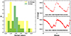 |
Fig. 1. Period distribution of the observed BL Her stars in the LMC with and without the presence of the bump feature in their G band light curve structure. Examples of BL Her stars exhibiting no bump or a bump in their light curves are displayed in the upper-right and lower-right panels, respectively. |
3. Description of the light curve parameters
We study the light curve structure of the BL Her stars using the Fourier decomposition technique. The theoretical and observed light curves in the Gaia passbands are fitted with the Fourier sine series (see, for example, Deb & Singh 2009; Das et al. 2020) of the form
 (1)
(1)
where x is the pulsation phase, m0 is the mean magnitude, and N is the order of the fit. The theoretical light curves are fitted with N = 20. For observed light curves, an optimum value of N is important so as not to fit the noise with an N too large or include systematic deviations with an N too small. To this end, we use the Baart’s condition (Baart 1982) and vary N from 4 to 8 to obtain the optimum order of fit. However, if we have a good phase coverage, we can use a reasonably higher order of fit (N ≤ 8) without running into the risk of over-fitting. This allows us to obtain higher-order Fourier parameters (described below), which in turn helps us constrain observed-model pairs better. The 35 BL Her stars that do not exhibit bumps are fitted with the order of fit N as obtained from the Baart’s condition. Of the 23 BL Her stars that exhibit bumps, 13 BL Her stars have a good phase coverage and are fitted with N = 7 while the rest 10 are fitted with the optimum order of fit using the Baart’s condition.
3.1. Fourier parameters
The Fourier amplitude and phase coefficients (Ak and ϕk) are used to obtain the Fourier amplitude and phase parameters, respectively, as follows:
 (2)
(2)
where k > 1 and 0 ≤ ϕk1 ≤ 2π.
3.2. Amplitude
The peak-to-peak amplitude, A, of the light curve is defined as the difference in the minimum and the maximum of the light variations:
 (3)
(3)
where (Mλ)min and (Mλ)max are the minimum and maximum magnitudes obtained from the Fourier fits in the λ band, respectively.
3.3. Skewness and acuteness
We also used a robust definition for the skewness of light curve, which is unaffected by the presence of bumps. The definition of skewness is as follows (Elgar 1987):
 (4)
(4)
where m is the mean-reduced light curve of the star, the brackets denote the mean over one pulsation period3. ℋ is the Hilbert transformation (Duoandikoetxea 2001, Chapter 3).
Acuteness is defined as the ratio of the phase duration of magnitude fainter than the mean magnitude to that of magnitude brighter than the mean magnitude (Stellingwerf & Donohoe 1987):
 (5)
(5)
where ϕfw is the phase duration of the magnitude, which is brighter than the mean magnitude (equal to the full width at half maximum of the light curve).
4. Estimating the stellar parameters of BL Her stars in the LMC
We next compared the theoretical and observed G band light curve structure of the BL Her stars in the LMC that have similar pulsation periods. We note that we carried out the comparison for all observed BL Her stars in the LMC with the complete set of BL Her models across the four sets of convection parameters. This allowed the possibility for stars with different effective temperatures to prefer models with different convection parameters, following the work of Kovács et al. (2023), who calibrated Teff-dependent convective parameters for RRab stars in M3.
4.1. BL Her stars with no bumps
Higher-order Fourier amplitude parameters capture the bump feature in light curves. Therefore, to find the best-fit matches for stars that do not exhibit bumps in their light curves, we restrict our model sample to stars where the higher-order Fourier amplitude parameters do not exceed
 (6)
(6)
where 8 ≤ k ≤ 11. Limiting the higher-order Fourier amplitude parameters rejects the BL Her models with bumps while still retaining BL Her models that can be matched with BL Her stars exhibiting the characteristic saw-tooth light curves without bumps.
Next, we constrain the sample of models with pulsation periods and amplitudes similar to those from observed BL Her stars in the LMC using the condition
 (7)
(7)
where Pmod and Pobs are the theoretical and the observed pulsation periods, respectively, and Amod and Aobs are the theoretical and the observed peak-to-peak amplitudes in the G band, respectively.
For a rigorous comparison, it is useful to construct a mathematically robust definition of the goodness-of-fit for each observed-model pair (see, for example, Smolec et al. 2013; Joyce et al. 2023). We define a parameter d to compute the offsets for each observed-model pair i with respect to their pulsation periods and over their Fourier parameter space as follows (see Smolec et al. 2013):
 (8)
(8)
where p ∈ {log(P),A, Sk, Ac, R21, R31, ϕ21, ϕ31} for the theoretical (pi, mod) and observed (pi, obs) light curves, with np as the weights for each parameter. While the rest of the parameters have equal weights of np = 1, the amplitude (A) and the skewness (Sk) of the light curve need a considerably higher weight of np = 10 to ensure that we obtain the best matches between models and observations.
Smolec et al. (2013) had equal weights of np = 1 for all light curve parameters involved in the determination of the parameter d. The reason for including a higher weight of np = 10 on the amplitude and skewness parameters in this work follows from the results obtained after carrying out a few exercises with different weights on A and Sk (see Fig. B.1 for more) where we found that a higher weight of np = 10 on the A and Sk parameters results in better matches of observed-model pairs as compared to using np = 1 or np = 5. Increasing the weight on the A and Sk parameters to np = 20 does not improve the observed-model pairs further. In addition, we also tested a higher weight of np = 10 on the pulsation period log(P) and found that it results in the same matches as with np = 1; this is likely because we had already placed a strong constraint on the pulsation period, |log(P)mod − log(P)obs|≤0.01, to begin with. We would like to highlight here that while the light curve optimization method adopted in this work is quite robust and we encourage readers to adopt this approach for similar work, the weights np on the light curve parameters should be decided after testing what works best for a particular dataset.
4.2. BL Her stars with bumps
For a comparison of the BL Her stars with bumps in their G band light curves, we used the complete set of BL Her models without any constraint on their higher-order Fourier amplitude parameters (Rk1). We have placed the same constraints on the models with respect to their pulsation periods and amplitudes as in Eq. (7). The parameter d that is used to quantify the offsets for each observed-model pair with respect to their pulsation periods and over their Fourier parameter space remains the same as in Eq. (8). However, the different parameter spaces are defined as follows:
 (9)
(9)
for the observed light curves fitted with the optimum order of fit from Baart’s condition and
 (10)
(10)
for the observed light curves fitted with N = 7. For both cases, the amplitude (A) and the skewness (Sk) of the light curve have a higher weight of np = 10 while the rest of the parameters have equal weights of np = 1.
Using as many light curve parameters as possible in determining d results in obtaining more precise and accurate observed-model pairs. Ideally, we want to include higher-order Fourier parameters for all the cases. However, limitations on the observed light curves (for example, not enough epochs or gaps in the epoch photometry) do not always allow us to fit observed light curves with a high order of harmonics, and we limited our conditions to include up to R31 and ϕ31 in such cases. For good quality light curves (and especially to capture the bump feature), we fitted the observed light curves with N = 7, wherever possible and thereby used parameters up to R71 (in Eq. 10). Since the bump feature is already well captured by higher-order Fourier amplitude parameters, we did not include the higher-order Fourier phase parameters. In Fig. B.2, for the particular case of Gaia DR3 4657865541316025600, we observe the need for including higher-order Fourier amplitude parameters up to R71 while not necessarily including higher-order Fourier phase parameters up to ϕ71.
4.3. Obtaining the best-matched observed-model pairs
Using the above-mentioned conditions, we obtained the score d for each observed-model pair. The smaller the score d, the smaller the offset for each observed-model pair with respect to their pulsation periods and over their Fourier parameter space. Thereafter, for each of the 58 BL Her stars, we short-listed ten corresponding models across all four sets of convection parameters that have the smallest d scores. We note that while most stars had at least ten corresponding models each, a few stars did not, owing to period and amplitude constraints. We investigate the degeneracy in the input stellar parameters of the BL Her models resulting in similar pulsation periods and light curve structure in Sect. 7; however, for estimating the stellar parameters and the distance to the LMC, we proceeded with the single best observed-model pairs.
In the final stage of the model fitting, the score d has small differences among the ten best observed-model pairs corresponding to a particular observed BL Her star. For this reason, we chose the final best-fit via the Kolmogorov-Smirnov goodness-of-fit test (Kolmogorov 1933; Smirnov 1948), which tests whether the normalized residuals are from a standard normal distribution (Andrae et al. 2010). This in practice means that we calculated the residuals from the observed (oi) and theoretical (mi) light curves, and normalized it with the corresponding observational error (σi):
 (11)
(11)
Under the hypothesis that the errors originate from observational errors only, the ri sample has to follow normal distribution (with 0 mean and a standard deviation of 1) for a perfect fit. In practice, due to the fact that the calculation is done on a model grid and secondary light curve features are difficult to be modeled (Marconi 2017), most of the cases do not have a goodness-of-fit above acceptance level. However, the observed-model pair that exhibits the largest goodness-of-fit score can be chosen as the best fit result (Andrae et al. 2010).
Finally, we verified the best-matched observed-model pairs corresponding to the 58 BL Her stars in the LMC by visual inspection. As mentioned earlier, while the complete set of BL Her models was used for comparison with the BL Her stars in the LMC, we chose the lower stellar mass models (M ≤ 0.65 M⊙) wherever possible due to their better fit to the observed stars. An excerpt of the light curves of the 30 accepted observed-model pairs with superior model fitting are displayed in Fig. 2 (the full image is shown in Fig. B.3); these 30 comprise our “gold sample”, which we analyzed further. Another 18 accepted observed-model pairs but with inferior model fitting (especially with respect to their amplitudes or skewness) are displayed in Fig. B.4 and labeled the “silver sample”. For the models that exhibit slightly higher amplitudes as compared to observed light curves, increasing the mixing length parameter may result in smaller pulsation amplitudes (see Di Criscienzo et al. 2004; Paxton et al. 2019, among others). The uncertainties on the convection parameters also affect the theoretical light curve amplitudes (Fiorentino et al. 2007). We therefore plan to calibrate the convection parameters for BL Her models in a future project as was done for RR Lyrae stars (Kovács et al. 2023, 2024). The light curves of 10 observed-model pairs rejected from further analysis are shown in Fig. B.5. An important thing to note here is that this analysis uses the four convection parameter sets as outlined in Paxton et al. (2019); however, these convection parameter values are merely useful starting choices and may be reasonably changed to obtain better fitted models for a particular observed light curve. It is therefore potentially possible to obtain MESA-RSP models with much better fits for the 10 rejected BL Her stars in Fig. B.5 and those will be targets of a future study.
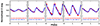 |
Fig. 2. Subsample of the light curves (normalized with respect to their mean magnitudes) of the gold sample BL Her stars in the LMC (in red) with their best-matched models (in blue). The full image is displayed in Fig. B.3. The input stellar parameters of the corresponding models are included in the format (Z, M/M⊙, L/L⊙, Teff, convection set) in each subplot. |
The estimated stellar parameters from the best-fit models corresponding to the 48 BL Her stars in the LMC are presented in Table A.2. These include the chemical composition (ZX), stellar mass (M), stellar luminosity (L), stellar radius (R), effective temperature (Teff), the convection parameter set used, and the measure of the final goodness-of-fit score for each observed-model pair. An interesting result is that the majority of the best-matched models corresponding to observed BL Her stars in the LMC are computed using the convection parameter sets A or C, with very few models computed using convection parameter sets B or D. We note that the convection parameter sets A and C are those without the radiative cooling. The other property that can be important about this parameter selection is that these two sets have the lowest eddy viscosity parameter (referred to as αm in Paxton et al. 2018). This parameter is 0.25 in set A and 0.4 in set C, while it is 0.5 in set B and 0.7 in set D. The eddy viscosity parameter controls the amount of kinetic energy converted into turbulent energy (Smolec & Moskalik 2008), thereby decreasing the velocity amplitude (Kovács et al. 2023), and also has a significant role in the damping of the pulsation (Kovács et al. 2024). Disentangling the effects of various convective parameters on the BL Her light curves is beyond the scope of this present study and is planned for the future. We note in passing that lowering the eddy viscosity parameter may also lead to the occurrence of more complex dynamical behavior in nonlinear models as well, ranging from period doubling to low-dimensional chaos. This was detected not only in BL Her but also in W Vir and RR Lyrae models (Smolec & Moskalik 2012, 2014; Smolec 2016; Kolláth et al. 2011; Molnár et al. 2012).
We further investigated the distribution of the subset of the gold sample of 30 BL Her models that match the best with BL Her stars in the LMC as a function of metallicity ([Fe/H]), stellar mass (M/M⊙), stellar luminosity (L/L⊙), effective temperature, and the convection parameter sets (see Fig. 3). As noted above, the majority of the models (93.3%) prefer the convection parameter sets A and C. In Paper II, we found the observed Fourier parameters in the G band from the BL Her stars in the LMC to overlap well with the theoretical Fourier parameter space from the low-mass models; a detailed light curve comparison between models and observations reveals that 90% of the best-matched BL Her models are low-mass models (≤0.65 M⊙). Only one model in the subset of best-matched BL Her models reach stellar luminosity higher than 200 L⊙. 66.7% of these BL Her models belong to the regime of the high-metallicity models ([Fe/H] ≥ −0.5). Most of the BL Her models lie near the blue edge of the instability strip, with 63.3% of the models having effective temperatures between 6400 and 6700 K. A similar distribution of the subset of the gold and silver samples of the BL Her models that match the best with BL Her stars in the LMC as as a function of [Fe/H], M/M⊙, L/L⊙, Teff and the convection parameter sets is displayed in Fig. B.6.
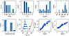 |
Fig. 3. Visualization of the properties of the gold sample of 30 BL Her models that match the best with BL Her stars in the LMC. Top panels: Histograms of the distribution of the BL Her models as a function of stellar mass (M/M⊙), stellar luminosity (L/L⊙), metallicity ([Fe/H]), effective temperature (Teff), and the convection parameter sets, respectively. The location of the subset of BL Her models is also depicted on the Hertzsprung-Russell diagram; the red and blue edges of the instability strip are estimated from the linear stability analysis from Paper I. Bottom panel: PW and PR relations of the 30 BL Her models, respectively. |
An alternate classification of pulsating variables with periods between 1 and 3 days was provided by Diethelm (1983, 1990) and Sandage et al. (1994) and a possible correlation between light curve type and mean metallicity was probed thereafter. These stars were called above-horizontal-branch (AHB) variables and based on the light curve morphology, they were subdivided into three classes – AHB1, AHB2, and AHB3 (for more details, see the example light curves provided in Diethelm 1983). The 6 BL Her stars with bumps in our gold sample exhibit their bump features on the ascending branch of the light curves, typical of the AHB2 class. From Table A.2, we find that 3 of them have Z = 0.00424 ([Fe/H] = −0.5) and another has Z = 0.00834 ([Fe/H] = −0.2). This is in agreement with Diethelm (1990) where they found the AHB2 stars to be moderately metal-poor with −0.7 ≤ [Fe/H] ≤ −0.1. However, our sample also has two bump light curves that have estimated metallicities outside of this range with Z = 0.00043 ([Fe/H] = −1.5) and Z = 0.013 ([Fe/H] = 0).
5. Validating estimated BL Her models with the OGLE database
To validate the stellar parameters estimated for the observed BL Her stars in the LMC (see Table A.2), we studied the color-magnitude diagram (CMD) of the observed-model pairs but using the OGLE observations of the observed BL Her stars. This is presented in Fig. 4. We made use of the optical (VI) light curves of T2Cs (and classical Cepheids) in the LMC from the OGLE-IV catalog to obtain the observed CMD (Soszyński et al. 2015, 2018). To account for interstellar extinction, we used the E(V − I) color excess values from the reddening map of Skowron et al. (2021), which is designed specifically for the Magellanic Clouds. We then transformed them to E(B − V) color excess values using E(V − I) = 1.38 × E(B − V) (Tammann et al. 2003). We finally obtained the extinction coefficients AV, AI using the following conversion factors from Schlegel et al. (1998):
 (12)
(12)
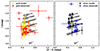 |
Fig. 4. CMD of the gold sample (left) and the silver sample (right) of the BL Her observed-model pairs using the OGLE counterparts. The gray points in the background represent all BL Her models from the four sets of convection parameters. |
The extinction-corrected I band apparent magnitudes are then converted to their respective absolute magnitudes using a distance modulus of μLMC = 18.477 ± 0.004 (statistical) ± 0.026 (systematic) from Pietrzyński et al. (2019), which is the present best-estimate of the geometrical distance to the LMC obtained by using 20 eclipsing binary systems and is precise to 1%. The uncertainties on the observed CMD take into account errors from the reddening map, the errors on the mean VI magnitudes, and the errors on the estimated LMC distance modulus.
The theoretical CMD is obtained by using the absolute VI magnitudes of the best-fit models (see Paper I), and the associated errors are estimated using Gaussian error propagation, with a luminosity step size of ±25 L⊙ of the computed grid of BL Her models. A comparison of the theoretical and observed I band light curves of the gold sample is displayed in Fig. B.7.
From Fig. 4, we find that the gold sample of 30 BL Her observed-model pairs in the (V − I) versus I CMD plane match reasonably well, especially for the bluer stars with (V − I) < 0.62. While BL Her models do exist for (V − I) > 0.62, we do not find good matches with the observed BL Her stars in this range. This seems like a current limitation of our model-fitting technique, where parameters for bluer stars are estimated better than that of red stars. We note that the choice of convection parameters plays a huge role in the stellar pulsation models (and subsequently their light curves), especially toward the red edge of the instability strip (Deupree 1977; Stellingwerf 1982a,b). The comparison of the theoretical and observed CMD of the silver sample of 18 BL Her observed-model pairs show that the BL Her models are offset from the observed BL Her stars. We therefore proceeded with the gold sample of 30 BL Her observed-model pairs only in the subsequent analysis for distance estimation to the LMC.
6. Estimating the distance to the LMC
As a direct application of our comparative analysis between theoretical and observed light curves of BL Her stars, we used the absolute Wesenheit magnitudes from the models and the apparent Wesenheit magnitudes from the observed BL Her stars in the LMC to estimate the distance modulus to the LMC.
As mentioned before, the comparison of the theoretical light curves with those from the observed BL Her stars in the LMC was carried out using the G band light curves only, since the empirical light curves contain better photometric data with a good phase coverage as compared to those in the GBP and GRP passbands. We did not correct for extinction in this present study. The light curve structure itself is not affected by extinction correction, or lack thereof. However, comparing the observed apparent magnitudes without extinction correction with the absolute magnitudes from the models using the light curves in the G band only would affect our estimation of the distance modulus to the LMC. In light of this, we made use of the observed-model pairs that exhibit best matches with respect to their pulsation periods and G band light curve structure but obtained their corresponding Wesenheit magnitudes, as defined by Ripepi et al. (2019) for Gaia DR3:
 (13)
(13)
where G, GBP, and GRP are the mean magnitudes in the respective Gaia passbands. The Wesenheit magnitudes for the observed BL Her stars are calculated using the mean GGBPGRP magnitudes as provided in the Gaia DR3 database4.
Wesenheit magnitudes offer the advantage of being minimally affected by the uncertainties arising from reddening corrections (Madore 1982). However, they are quite sensitive to the extinction law assumed. The extinction law of the LMC has been quite extensively studied (Gordon et al. 2003; Gao et al. 2013; Wang & Chen 2023, among others), thereby justifying our use of Wesenheit magnitudes as reddening-free magnitudes in this work. The Wesenheit magnitudes obtained from the theoretical and the observed light curves for the best-matched observed-model pairs are included in Table A.2; these are thereby used to estimate the individual distance moduli μ to the LMC. The distribution of the individual distance moduli as a function of the pulsation period and the metal abundance is displayed in the upper left-hand panel of Fig. 5. The variation in the distance moduli with metal abundance (slope = −0.052 ± 0.103 with a scatter of σ = 0.363) is presented in the lower left-hand panel of Fig. 5; however, given the small sample, we cannot claim to have found any conclusive evidence of a correlation between the two.
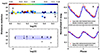 |
Fig. 5. The individual distance moduli to the LMC estimated using the gold sample of 30 BL Her observed-model pairs. Left: Variation in distance modulus as a function of period (top) and metal abundance (bottom). Solid lines represent μLMC = 18.477 ± 0.026 (Pietrzyński et al. 2019) in the top panel and best-fitting linear regression in the bottom panel, while the dashed lines represent 1σ errors in each case. Right: Theoretical and observed (normalized with respect to the mean magnitude) G band light curves of two BL Her stars that are consistent on the Fourier plane. |
Finally, we obtained an average distance modulus to the LMC of μLMC = 18.582 ± 0.067 using the gold sample of 30 best-matched observed-model pairs, as summarized in Table A.2. As mentioned before, Pietrzyński et al. (2019) provides the most accurate and precise measurement of the geometrical distance to the LMC to date of μLMC = 18.477 ± 0.004 (statistical) ± 0.026 (systematic). Wielgórski et al. (2022) used the PL relations of Milky Way T2Cs to obtain a distance modulus of μLMC = 18.540 ± 0.026 (statistical) ± 0.034 (systematic). Our results are therefore in reasonably good agreement with published results and lie within the bounds of the above-quoted literature values.
The period-Wesenheit (PW) relation for the subset of the best-matched gold sample of 30 BL Her models is displayed in the lowest panel of Fig. 3 and exhibits a slope of −2.805 ± 0.164 with a scatter of σ = 0.115. For comparison, the empirical PW relation for the 58 BL Her stars in the LMC has a slope of −2.398 ± 0.146 with a scatter of σ = 0.144 (see Table 5 of Paper II). The T statistic5 and its associated probability p(t) of acceptance of the null hypothesis (equal slopes) obtained for the comparison of the two linear regression slopes under the two-tailed t-distribution are 1.854 and 0.067, respectively, thereby suggesting statistically similar PW relations.
The PR relation for the subset of the best-matched gold sample of 30 BL Her models is also presented in the lowest panel of Fig. 3 and exhibits a slope of 0.565 ± 0.035 with a scatter of σ = 0.025. This is in excellent agreement with the empirical PR slope of 0.564 ± 0.049 with a scatter of σ = 0.047 from the BL Her stars in the LMC (Groenewegen & Jurkovic 2017). The (|T|, p(t)) values for the comparison of the two linear regression slopes are (0.017, 0.987).
7. One star, many models
So far, we have discussed the results from the best-matched model corresponding to a particular observed star. However, as mentioned in Sect. 4.3, we short-listed ten models each that match the closest with an observed BL Her star with respect to their pulsation periods and their Fourier parameter space. In this section we study the degeneracy in the input stellar parameters of the BL Her models that result in similar pulsation periods and light curve structure. An example of the ten best-matched models corresponding to one particular observed BL Her star without bump, Gaia DR3 4661638790215403008, is displayed in Fig. 6, along with the input stellar parameters of the corresponding models in each subplot. We also study the correlations of the different stellar parameters – chemical composition Z, stellar mass M/M⊙, stellar luminosity L/L⊙, stellar radius log(R/R⊙) and effective temperature Teff – of the ten best-matched models corresponding to the star in Fig. 7. While the stellar mass is restricted to the range M/M⊙ ∈ [0.5, 0.65], with a fixed stellar luminosity L/L⊙ = 100, the effective temperature is quite broad in the range Teff ∈ [6550, 6800] (K). There is also a wide range of chemical compositions with Z ∈ {0.00014, 0.00043, 0.00061, 0.00424, 0.00834, 0.013}. However, the majority of the models (80%) still prefer the convection parameter sets A and C.
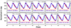 |
Fig. 6. Example of the ten best-matched models corresponding to one particular observed BL Her star, Gaia DR3 4661638790215403008. The observed light curve is shown in red and the theoretical light curves in blue. The input stellar parameters of the corresponding models are included in the format (Z, M/M⊙, L/L⊙, Teff, convection set) in each subplot. |
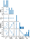 |
Fig. 7. Corner plot exhibiting the correlations of the different stellar parameters (chemical composition Z, stellar mass M/M⊙, stellar luminosity L/L⊙, stellar radius log(R/R⊙), and effective temperature Teff) using the ten best-matched models corresponding to one particular observed BL Her star, Gaia DR3 4661638790215403008. |
An example of the ten best-matched models corresponding to the observed BL Her star with bump, Gaia DR3 4658440315161900928, and the correlations of the different stellar parameters are displayed in Figs. B.8 and B.9, respectively. The stellar mass is restricted to the range M/M⊙ ∈ [0.65, 0.75] with a fixed stellar luminosity L/L⊙ = 150 and the effective temperature in the range of Teff ∈ [6000, 6150] (K). The chemical composition cannot be constrained, as the ten best-matched models span the entire range of the input parameter used in the grid with Z ∈ {0.00014, 0.00043, 0.00061, 0.00135, 0.00424, 0.00834, 0.013}. Once again, the majority of the models (70%) still prefer the convection parameter set C.
This analysis was carried out to show that while the stellar estimates provided in Table A.2, using our robust light-curve-fitting approach, are reasonably good (especially for the gold sample BL Her observed-model pairs), one has to be careful because degeneracies exist in the models that may result in similar pulsation periods and light curve structure. A way to constrain the observed-model pairs further would be to simultaneously fit the light curves and the radial velocity curves for stars and models that have similar pulsation periods. The two examples above also suggest that while the metallicity range may be difficult to constrain, one could recompute new models by adopting the weighted averaged values of M, L, and Teff (with the weights scaled according to their goodness-of-fit scores) of the ten best observed-model pairs, keeping the ZX and convection parameter sets the same. Thereafter, a second iteration of the comparison of the observed and the new modeled light curves may help constrain the input stellar parameters (and especially, the metallicity) of the models better. However, we note that this study is the most robust light-curve fitting that can be done at present for BL Her stars using the latest available observations from Gaia DR3 and the most recent stellar pulsation models. We also plan to constrain the convection parameters for BL Her models in a future project, similar to what has been carried out for RRab (Kovács et al. 2023) and RRc stars (Kovács et al. 2024).
8. Summary and conclusion
We carried out an extensive comparison of the light curve structure of BL Her stars in the G band using observations from Gaia DR3 (Gaia Collaboration 2016, 2023) and the most recent stellar pulsation models computed for a wide range of input parameters – metallicity (−2.0 dex ≤ [Fe/H] ≤ 0.0 dex), stellar mass (0.5 M⊙–0.8 M⊙), stellar luminosity (50 L⊙–300 L⊙), and effective temperature (full extent of the instability strip; in steps of 50 K) – typical for BL Her stars using MESA-RSP (Paper I; Paper II). The important results from this analysis are summarized below:
-
We compared the G band theoretical light curves of the complete set of BL Her models computed using the different convection parameter sets with the observed light curves of the BL Her stars in the LMC that have similar pulsation periods. We used the mathematically robust goodness-of-fit measure over the Fourier parameter space to obtain best-fit models for 48 stars in the LMC and provide the stellar parameter estimates in Table A.2.
-
We find a relatively flat distribution of stellar masses between 0.5 and 0.65 M⊙. Although 90% of models fall into this range, we found three stars where the fits clearly preferred a higher mass of 0.75 M⊙.
-
An interesting result is that while there was no obvious preference in the choice of convection parameter sets in Paper II, when we compared the theoretical and empirical PW relations of BL Her stars at mean light, an extensive light curve comparison analysis shows that the majority of the best-matched models are computed using the convection parameter sets A and C. We note that the convection parameter sets A and C are not only computed without radiative cooling, but also have low eddy viscosities. The result that the majority of the best-matched models are computed using sets A and C could be an interplay of the different convective parameters and does not allow us to conclude that radiative cooling is inefficient in these models.
-
The PW relation for the subset of the best-matched gold sample of 30 BL Her models has a slope of −2.805 ± 0.164, which is in good agreement with the empirical PW slope of −2.398 ± 0.146 from the BL Her stars in the LMC (using data from Gaia DR3 in Paper II). We also found the PR relation for the gold sample of 30 BL Her models to have a slope of 0.565 ± 0.035, in excellent agreement with the empirical PR slope of 0.564 ± 0.049 from the BL Her stars in the LMC (Groenewegen & Jurkovic 2017).
-
We used the Wesenheit magnitudes of the subset of the 30 best-matched observed-model pairs to estimate a distance modulus to the LMC of μLMC = 18.582 ± 0.067, which lies within the bounds of previous literature values from Pietrzyński et al. (2019) and Wielgórski et al. (2022).
-
We also analyzed the degeneracy in the stellar parameters of the BL Her models that result in similar pulsation periods and light curve structure and noted that an even more robust method of fitting would be to simultaneously fit multiband light curves and radial velocity curves for stars and models that have similar pulsation periods. However, we note that this study is the most robust light-curve-fitting that can be done at present using the most recent theoretical and observed data.
-
Despite the large number of BL Her models, we did not find best-fit models for ten BL Her stars in the LMC. A possible explanation could be the “curse of dimensionality” (Bellman & Kalaba 1959), which suggests that the number of configurations (in this work: pulsation period, light curve amplitude, and Fourier parameters) covered by an observation decreases as the dimensionality or parameter space of the models increases. Another reason is that this analysis uses the four convection parameter sets as outlined in Paxton et al. (2019); however, these convection parameter values are merely useful starting points. Our grid of models suggests that the choice of convection parameters clearly plays an important role in the theoretical light curve structure, especially the Fourier amplitude parameters, and, therefore, may be reasonably changed to obtain better fitted models for a particular observed light curve.
Our analysis successfully demonstrates that in the era of percent-level precision in the calibration of PL relations of classical pulsators, it is extremely important to not just compare the observations and the stellar pulsation models at mean light but also compare their light curves over a complete pulsation cycle for better constraints on the stellar pulsation theory. The extensive light curve comparison analysis shows a clear preference for radial stellar pulsation models computed without radiative cooling for BL Her stars using MESA-RSP. However, as mentioned earlier, this does not allow us to conclude that radiative cooling is inefficient in these models; it could be the result of an interplay between the various convective parameters. It is therefore important to calibrate the convection parameters as was done for RRab (Kovács et al. 2023) and RRc stars (Kovács et al. 2024), and therefore we plan to constrain the convection parameters for BL Her models in a future project. We would like to highlight here that adopting static model atmospheres while the pulsating atmosphere is clearly dynamic may also affect our extensive light curve analysis comparison of observed and theoretical light curves.
The low-mass models, M/M⊙ ∈ [0.5, 0.6], were computed with stellar luminosity L/L⊙ ∈ ⟨50,200⟩ only.
The fractional growth of the kinetic energy per pulsation period Γ does not vary by more than 0.01, the amplitude of radius variation ΔR by more than 0.01 R⊙, and the pulsation period P by more than 0.01 d over the last 100 cycles of the completed integration (see Fig. 2 of Paper I for a detailed pictorial representation).
In general, this should be for a large number of periods, but since we work with the Fourier series, there is no cycle-to-cycle variation.
We defined a T statistic for the comparison of two linear regression slopes,  with sample sizes, n and m, respectively, as follows:
where  is the variance of the slope. The null hypothesis of equivalent slopes is rejected if T > tα/2, ν (or the probability of the observed value of the T statistic) is p < 0.05, where tα/2, ν is the critical value under the two-tailed t-distribution with 95% confidence limit (α = 0.05) and degrees of freedom, ν = n + m − 4.
Acknowledgments
The authors thank the referee for useful comments and suggestions that improved the quality of the manuscript. This research was supported by the KKP-137523 ‘SeismoLab’ Élvonal grant and by the NKFIH excellence grant TKP2021-NKTA-64 of the Hungarian Research, Development and Innovation Office (NKFIH). M.J. gratefully acknowledges funding from MATISSE: Measuring Ages Through Isochrones, Seismology, and Stellar Evolution, awarded through the European Commission’s Widening Fellowship. This project has received funding from the European Union’s Horizon 2020 research and innovation program. RS is supported by the Polish National Science Centre, SONATA BIS grant, 2018/30/E/ST9/00598. This research was supported by the International Space Science Institute (ISSI) in Bern/Beijing through ISSI/ISSI-BJ International Team project ID #24-603 – “EXPANDING Universe” (EXploiting Precision AstroNomical Distance INdicators in the Gaia Universe). The authors acknowledge the use of High Performance Computing facility Pegasus at IUCAA, Pune as well as at the HUN-REN (formerly ELKH) Cloud and the following software used in this project: MESA r11701 (Paxton et al. 2011, 2013, 2015, 2018, 2019; Jermyn et al. 2023). This research has made use of NASA’s Astrophysics Data System.
References
- Andrae, R., Schulze-Hartung, T., & Melchior, P. 2010, ArXiv e-prints [arXiv:1012.3754] [Google Scholar]
- Asplund, M., Grevesse, N., Sauval, A. J., & Scott, P. 2009, ARA&A, 47, 481 [NASA ADS] [CrossRef] [Google Scholar]
- Baart, M. L. 1982, IMA J. Numer. Anal., 2, 241 [CrossRef] [Google Scholar]
- Beaton, R. L., Freedman, W. L., Madore, B. F., et al. 2016, ApJ, 832, 210 [Google Scholar]
- Bellinger, E. P., Kanbur, S. M., Bhardwaj, A., & Marconi, M. 2020, MNRAS, 491, 4752 [NASA ADS] [CrossRef] [Google Scholar]
- Bellman, R., & Kalaba, R. 1959, IRE Trans. Autom. Control, 4, 1 [CrossRef] [Google Scholar]
- Bhardwaj, A., Kanbur, S. M., Marconi, M., et al. 2017a, MNRAS, 466, 2805 [NASA ADS] [CrossRef] [Google Scholar]
- Bhardwaj, A., Rejkuba, M., Minniti, D., et al. 2017b, A&A, 605, A100 [NASA ADS] [CrossRef] [EDP Sciences] [Google Scholar]
- Bhardwaj, A., Kanbur, S. M., Rejkuba, M., et al. 2022, A&A, 668, A59 [NASA ADS] [CrossRef] [EDP Sciences] [Google Scholar]
- Bono, G., Caputo, F., & Santolamazza, P. 1997, A&A, 317, 171 [NASA ADS] [Google Scholar]
- Bono, G., Castellani, V., & Marconi, M. 2000, ApJ, 532, L129 [Google Scholar]
- Bono, G., Castellani, V., & Marconi, M. 2002, ApJ, 565, L83 [Google Scholar]
- Bono, G., Braga, V. F., Fiorentino, G., et al. 2020, A&A, 644, A96 [NASA ADS] [CrossRef] [EDP Sciences] [Google Scholar]
- Braga, V. F., Bono, G., Fiorentino, G., et al. 2020, A&A, 644, A95 [NASA ADS] [CrossRef] [EDP Sciences] [Google Scholar]
- Buchler, J. R., & Moskalik, P. 1992, ApJ, 391, 736 [NASA ADS] [CrossRef] [Google Scholar]
- Buchler, J. R., Moskalik, P., & Kovacs, G. 1990, ApJ, 351, 617 [NASA ADS] [CrossRef] [Google Scholar]
- Caputo, F. 1998, A&ARv, 9, 33 [NASA ADS] [CrossRef] [Google Scholar]
- Das, S., Bhardwaj, A., Kanbur, S. M., Singh, H. P., & Marconi, M. 2018, MNRAS, 481, 2000 [CrossRef] [Google Scholar]
- Das, S., Kanbur, S. M., Bellinger, E. P., et al. 2020, MNRAS, 493, 29 [NASA ADS] [CrossRef] [Google Scholar]
- Das, S., Kanbur, S. M., Smolec, R., et al. 2021, MNRAS, 501, 875 [Google Scholar]
- Das, S., Molnár, L., Kanbur, S. M., et al. 2024, A&A, 684, A170 [NASA ADS] [CrossRef] [EDP Sciences] [Google Scholar]
- Deb, S., & Singh, H. P. 2009, A&A, 507, 1729 [NASA ADS] [CrossRef] [EDP Sciences] [Google Scholar]
- Deupree, R. G. 1977, ApJ, 211, 509 [NASA ADS] [CrossRef] [Google Scholar]
- Di Criscienzo, M., Marconi, M., & Caputo, F. 2004, ApJ, 612, 1092 [Google Scholar]
- Di Criscienzo, M., Caputo, F., Marconi, M., & Cassisi, S. 2007, A&A, 471, 893 [NASA ADS] [CrossRef] [EDP Sciences] [Google Scholar]
- Di Fabrizio, L., Clementini, G., Marconi, M., et al. 2002, MNRAS, 336, 841 [Google Scholar]
- Diethelm, R. 1983, A&A, 124, 108 [NASA ADS] [Google Scholar]
- Diethelm, R. 1990, A&A, 239, 186 [Google Scholar]
- Duoandikoetxea, J. 2001, Fourier Analysis (Providence: American Mathematical Society) [Google Scholar]
- Elgar, S. 1987, IEEE Transactions on Acoustics, Speech, and Signal Processing, 35, 1725 [Google Scholar]
- Feuchtinger, M. U., & Dorfi, E. A. 1997, A&A, 322, 817 [NASA ADS] [Google Scholar]
- Fiorentino, G., Marconi, M., Musella, I., & Caputo, F. 2007, A&A, 476, 863 [NASA ADS] [CrossRef] [EDP Sciences] [Google Scholar]
- Gaia Collaboration (Prusti, T., et al.) 2016, A&A, 595, A1 [NASA ADS] [CrossRef] [EDP Sciences] [Google Scholar]
- Gaia Collaboration (Vallenari, A., et al.) 2023, A&A, 674, A1 [NASA ADS] [CrossRef] [EDP Sciences] [Google Scholar]
- Gao, J., Jiang, B. W., Li, A., & Xue, M. Y. 2013, ApJ, 776, 7 [Google Scholar]
- Gingold, R. A. 1985, Mem. Soc. Astron. Ital., 56, 169 [Google Scholar]
- Gordon, K. D., Clayton, G. C., Misselt, K. A., Landolt, A. U., & Wolff, M. J. 2003, ApJ, 594, 279 [NASA ADS] [CrossRef] [Google Scholar]
- Groenewegen, M. A. T., & Jurkovic, M. I. 2017, A&A, 604, A29 [NASA ADS] [CrossRef] [EDP Sciences] [Google Scholar]
- Hinshaw, G., Larson, D., Komatsu, E., et al. 2013, ApJS, 208, 19 [Google Scholar]
- Jermyn, A. S., Bauer, E. B., Schwab, J., et al. 2023, ApJS, 265, 15 [NASA ADS] [CrossRef] [Google Scholar]
- Joyce, M., Johnson, C. I., Marchetti, T., et al. 2023, ApJ, 946, 28 [NASA ADS] [CrossRef] [Google Scholar]
- Jurcsik, J., & Kovacs, G. 1996, A&A, 312, 111 [Google Scholar]
- Keller, S. C., & Wood, P. R. 2002, ApJ, 578, 144 [Google Scholar]
- Keller, S. C., & Wood, P. R. 2006, ApJ, 642, 834 [Google Scholar]
- Kolláth, Z., Molnár, L., & Szabó, R. 2011, MNRAS, 414, 1111 [CrossRef] [Google Scholar]
- Kolmogorov, A. 1933, Giornale dell’ Istituto Italiano degli Attuari, 4, 83 [Google Scholar]
- Kovacs, G., & Kanbur, S. M. 1998, MNRAS, 295, 834 [CrossRef] [Google Scholar]
- Kovács, G. B., Nuspl, J., & Szabó, R. 2023, MNRAS, 521, 4878 [CrossRef] [Google Scholar]
- Kovács, G. B., Nuspl, J., & Szabó, R. 2024, MNRAS, 527, L1 [Google Scholar]
- Kumar, N., Bhardwaj, A., Singh, H. P., et al. 2024, MNRAS, 531, 2976 [NASA ADS] [CrossRef] [Google Scholar]
- Madore, B. F. 1982, ApJ, 253, 575 [NASA ADS] [CrossRef] [Google Scholar]
- Majaess, D. J. 2010, Journal of the American Association of Variable Star Observers, 38, 100 [Google Scholar]
- Marconi, M. 2017, Eur. Phys. J. Web Conf., 152, 06001 [NASA ADS] [CrossRef] [EDP Sciences] [Google Scholar]
- Marconi, M., & Clementini, G. 2005, AJ, 129, 2257 [Google Scholar]
- Marconi, M., & Degl’Innocenti, S. 2007, A&A, 474, 557 [EDP Sciences] [Google Scholar]
- Marconi, M., & Di Criscienzo, M. 2007, A&A, 467, 223 [EDP Sciences] [Google Scholar]
- Marconi, M., Molinaro, R., Ripepi, V., Musella, I., & Brocato, E. 2013a, MNRAS, 428, 2185 [Google Scholar]
- Marconi, M., Molinaro, R., Bono, G., et al. 2013b, ApJ, 768, L6 [Google Scholar]
- Marconi, M., Molinaro, R., Ripepi, V., et al. 2017, MNRAS, 466, 3206 [NASA ADS] [CrossRef] [Google Scholar]
- Marconi, M., De Somma, G., Molinaro, R., et al. 2024, MNRAS, 529, 4210 [NASA ADS] [CrossRef] [Google Scholar]
- Matsunaga, N., Fukushi, H., Nakada, Y., et al. 2006, MNRAS, 370, 1979 [Google Scholar]
- Matsunaga, N., Feast, M. W., & Menzies, J. W. 2009, MNRAS, 397, 933 [NASA ADS] [CrossRef] [Google Scholar]
- Matsunaga, N., Feast, M. W., & Soszyński, I. 2011, MNRAS, 413, 223 [Google Scholar]
- Molnár, L., Kolláth, Z., Szabó, R., et al. 2012, ApJ, 757, L13 [CrossRef] [Google Scholar]
- Moskalik, P., & Buchler, J. R. 1993, ApJ, 406, 190 [NASA ADS] [CrossRef] [Google Scholar]
- Nemec, J. M., Cohen, J. G., Ripepi, V., et al. 2013, ApJ, 773, 181 [CrossRef] [Google Scholar]
- Netzel, H., Molnár, L., & Joyce, M. 2023, MNRAS, 525, 5378 [NASA ADS] [CrossRef] [Google Scholar]
- Ngeow, C.-C., Bhardwaj, A., Henderson, J.-Y., et al. 2022, AJ, 164, 154 [NASA ADS] [CrossRef] [Google Scholar]
- Paxton, B., Bildsten, L., Dotter, A., et al. 2011, ApJS, 192, 3 [Google Scholar]
- Paxton, B., Cantiello, M., Arras, P., et al. 2013, ApJS, 208, 4 [Google Scholar]
- Paxton, B., Marchant, P., Schwab, J., et al. 2015, ApJS, 220, 15 [Google Scholar]
- Paxton, B., Schwab, J., Bauer, E. B., et al. 2018, ApJS, 234, 34 [NASA ADS] [CrossRef] [Google Scholar]
- Paxton, B., Smolec, R., Schwab, J., et al. 2019, ApJS, 243, 10 [Google Scholar]
- Petersen, J. O. 1980, Space Sci. Rev., 27, 495 [NASA ADS] [CrossRef] [Google Scholar]
- Pietrzyński, G., Graczyk, D., Gallenne, A., et al. 2019, Nature, 567, 200 [Google Scholar]
- Ripepi, V., Molinaro, R., Musella, I., et al. 2019, A&A, 625, A14 [NASA ADS] [CrossRef] [EDP Sciences] [Google Scholar]
- Ripepi, V., Clementini, G., Molinaro, R., et al. 2023, A&A, 674, A17 [NASA ADS] [CrossRef] [EDP Sciences] [Google Scholar]
- Sandage, A., Diethelm, R., & Tammann, G. A. 1994, A&A, 283, 111 [Google Scholar]
- Schlegel, D. J., Finkbeiner, D. P., & Davis, M. 1998, ApJ, 500, 525 [Google Scholar]
- Simon, N. R., & Davis, C. G. 1983, ApJ, 266, 787 [NASA ADS] [CrossRef] [Google Scholar]
- Simon, N. R., & Lee, A. S. 1981, ApJ, 248, 291 [NASA ADS] [CrossRef] [Google Scholar]
- Simon, N. R., & Teays, T. J. 1982, ApJ, 261, 586 [NASA ADS] [CrossRef] [Google Scholar]
- Skowron, D. M., Skowron, J., Udalski, A., et al. 2021, ApJS, 252, 23 [Google Scholar]
- Smirnov, N. 1948, Ann. Math. Stat., 19, 279 [CrossRef] [Google Scholar]
- Smolec, R. 2005, Acta Astron., 55, 59 [NASA ADS] [Google Scholar]
- Smolec, R. 2016, MNRAS, 456, 3475 [NASA ADS] [CrossRef] [Google Scholar]
- Smolec, R., & Moskalik, P. 2008, Acta Astron., 58, 193 [NASA ADS] [Google Scholar]
- Smolec, R., & Moskalik, P. 2012, MNRAS, 426, 108 [NASA ADS] [CrossRef] [Google Scholar]
- Smolec, R., & Moskalik, P. 2014, MNRAS, 441, 101 [CrossRef] [Google Scholar]
- Smolec, R., Soszyński, I., Moskalik, P., et al. 2012, MNRAS, 419, 2407 [CrossRef] [Google Scholar]
- Smolec, R., Pietrzyński, G., Graczyk, D., et al. 2013, MNRAS, 428, 3034 [NASA ADS] [CrossRef] [Google Scholar]
- Soszyński, I., Udalski, A., Pietrukowicz, P., et al. 2011, Acta Astron., 61, 285 [NASA ADS] [Google Scholar]
- Soszyński, I., Udalski, A., Szymański, M. K., et al. 2015, Acta Astron., 65, 297 [NASA ADS] [Google Scholar]
- Soszyński, I., Udalski, A., Szymański, M. K., et al. 2018, Acta Astron., 68, 89 [NASA ADS] [Google Scholar]
- Stellingwerf, R. F. 1982a, ApJ, 262, 330 [NASA ADS] [CrossRef] [Google Scholar]
- Stellingwerf, R. F. 1982b, ApJ, 262, 339 [NASA ADS] [CrossRef] [Google Scholar]
- Stellingwerf, R. F., & Donohoe, M. 1987, ApJ, 314, 252 [NASA ADS] [CrossRef] [Google Scholar]
- Tammann, G. A., Sandage, A., & Reindl, B. 2003, A&A, 404, 423 [NASA ADS] [CrossRef] [EDP Sciences] [Google Scholar]
- Wang, S., & Chen, X. 2023, ApJ, 946, 43 [Google Scholar]
- Wielgórski, P., Pietrzyński, G., Pilecki, B., et al. 2022, ApJ, 927, 89 [CrossRef] [Google Scholar]
- Wood, P. R., Arnold, A. S., & Sebo, K. M. 1997, ApJ, 485, L25 [NASA ADS] [CrossRef] [Google Scholar]
Appendix A: Additional tables
In Table A.1 we present the equivalent ZX values for each [Fe/H] value. Table A.2 provides the estimated stellar parameters from the best-fit models corresponding to the 48 BL Her stars in the LMC.
Chemical compositions of the adopted pulsation models.
BL Her stars in the LMC with their corresponding best-matched MESA-RSP models.
Appendix B: Additional figures
In Fig. B.1 we exhibit the different observed-model pairs obtained from preliminary exercises carried out using different conditions to determine the robust weights on the light curve parameters for calculating the parameter d as in Eq. 8. The light curve parameters are p ∈ {log(P),A, Sk, Ac, Ri1, ϕi1} and the different conditions used are as follows:
-
Condition 1: np = 1 for all
-
Condition 2: np = 5 for A, Sk; np = 1 for the rest
-
Condition 3: np = 10 for A, Sk; np = 1 for the rest
-
Condition 4: np = 20 for A, Sk; np = 1 for the rest
-
Condition 5: np = 10 for log(P), A, Sk; np = 1 for the rest
The reason for placing higher weights on A and Sk (and not on the other parameters) arises from the fact that the theoretical and observed light curves in this work tended to be more “offset” in terms of either their amplitudes or their skewness; this is also evident from the silver sample. The reader is advised to set weights on the light curve parameters in the determination of the parameter d based on their datasets.
In Fig. B.2 we present the observed-model pairs obtained from using different conditions for the cases where the observed light curves were fitted with order of fit, N = 7. The different conditions used are as follows:
-
Condition 1: p ∈ {log(P),A, Sk, Ac, R21, R31, ϕ21, ϕ31}
-
Condition 2: p ∈ {log(P),A, Sk, Ac, R21, R31, R41, R51, R61, R71, ϕ21, ϕ31}
-
Condition 3: p ∈ {log(P),A, Sk, Ac, R21, R31, R41, R51, R61, R71, ϕ21, ϕ31, ϕ41, ϕ51, ϕ61, ϕ71}
Figures B.3 and B.4 display the light curves (normalized with respect to their mean magnitudes) of the BL Her stars in the LMC with their best-matched models for the gold sample and the silver sample, respectively. In Fig. B.5 we display the light curves of the ten observed-model pairs of BL Her stars that were rejected from this analysis. Figure B.6 shows the distribution of the subset of the gold sample and the silver sample of BL Her models that match the best with BL Her stars in the LMC as as a function of metallicity [Fe/H], stellar mass M/M⊙, stellar luminosity L/L⊙, effective temperature and the convection parameter sets. The I band light curves (normalized with respect to their mean magnitudes) of the gold sample BL Her observed-model pairs using the OGLE database is presented in Fig. B.7. Figures B.8 and B.9 present an example of the ten best-matched models corresponding to the observed BL Her star with bump, Gaia DR3 4658440315161900928, and the correlations of the different stellar parameters, respectively.
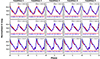 |
Fig. B.1. Visualization of the observed-model pairs obtained from preliminary exercises carried out using different conditions to determine the robust weights on the light curve parameters for calculating the parameter d as in Eq. 8. The input stellar parameters of the corresponding models are included in the format (Z, M/M⊙, L/L⊙, Teff, convection set) in each subplot. |
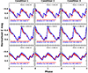 |
Fig. B.2. Visualization of the observed-model pairs obtained from using different conditions for the cases where the observed light curves were fitted with order of fit, N = 7. The input stellar parameters of the corresponding models are included in the format (Z, M/M⊙, L/L⊙, Teff, convection set) in each subplot. |
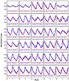 |
Fig. B.3. Light curves (normalized with respect to their mean magnitudes) of the 30 BL Her stars in the LMC (in red) with their best-matched models (in blue). These 30 accepted observed-model pairs are considered as the gold sample with superior model fitting. The input stellar parameters of the corresponding models are included in the format (Z, M/M⊙, L/L⊙, Teff, convection set) in each subplot. |
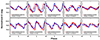 |
Fig. B.5. Light curves of the rejected model (blue)-observed (red) pairs of the 10 BL Her stars in the LMC. Note that the BL Her star Gaia DR3 4657832869370030720 has sparse epoch photometry in the G band. |
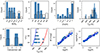 |
Fig. B.6. Same as Fig. 3 but for both the gold sample and the silver sample of the BL Her models. The open-faced histogram bars and circles represent the silver sample BL Her models. |
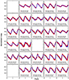 |
Fig. B.7. Same as Fig. B.3 but for their OGLE counterparts. Missing subplots indicate lack of their OGLE counterparts and/or lack of VI photometric data. |
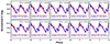 |
Fig. B.8. Same as Fig. 6 but for the observed BL Her star with the bump feature Gaia DR3 4658440315161900928. |
All Tables
BL Her stars in the LMC with their corresponding best-matched MESA-RSP models.
All Figures
|
Fig. 1. Period distribution of the observed BL Her stars in the LMC with and without the presence of the bump feature in their G band light curve structure. Examples of BL Her stars exhibiting no bump or a bump in their light curves are displayed in the upper-right and lower-right panels, respectively. |
| In the text | |
|
Fig. 2. Subsample of the light curves (normalized with respect to their mean magnitudes) of the gold sample BL Her stars in the LMC (in red) with their best-matched models (in blue). The full image is displayed in Fig. B.3. The input stellar parameters of the corresponding models are included in the format (Z, M/M⊙, L/L⊙, Teff, convection set) in each subplot. |
| In the text | |
|
Fig. 3. Visualization of the properties of the gold sample of 30 BL Her models that match the best with BL Her stars in the LMC. Top panels: Histograms of the distribution of the BL Her models as a function of stellar mass (M/M⊙), stellar luminosity (L/L⊙), metallicity ([Fe/H]), effective temperature (Teff), and the convection parameter sets, respectively. The location of the subset of BL Her models is also depicted on the Hertzsprung-Russell diagram; the red and blue edges of the instability strip are estimated from the linear stability analysis from Paper I. Bottom panel: PW and PR relations of the 30 BL Her models, respectively. |
| In the text | |
|
Fig. 4. CMD of the gold sample (left) and the silver sample (right) of the BL Her observed-model pairs using the OGLE counterparts. The gray points in the background represent all BL Her models from the four sets of convection parameters. |
| In the text | |
|
Fig. 5. The individual distance moduli to the LMC estimated using the gold sample of 30 BL Her observed-model pairs. Left: Variation in distance modulus as a function of period (top) and metal abundance (bottom). Solid lines represent μLMC = 18.477 ± 0.026 (Pietrzyński et al. 2019) in the top panel and best-fitting linear regression in the bottom panel, while the dashed lines represent 1σ errors in each case. Right: Theoretical and observed (normalized with respect to the mean magnitude) G band light curves of two BL Her stars that are consistent on the Fourier plane. |
| In the text | |
|
Fig. 6. Example of the ten best-matched models corresponding to one particular observed BL Her star, Gaia DR3 4661638790215403008. The observed light curve is shown in red and the theoretical light curves in blue. The input stellar parameters of the corresponding models are included in the format (Z, M/M⊙, L/L⊙, Teff, convection set) in each subplot. |
| In the text | |
|
Fig. 7. Corner plot exhibiting the correlations of the different stellar parameters (chemical composition Z, stellar mass M/M⊙, stellar luminosity L/L⊙, stellar radius log(R/R⊙), and effective temperature Teff) using the ten best-matched models corresponding to one particular observed BL Her star, Gaia DR3 4661638790215403008. |
| In the text | |
|
Fig. B.1. Visualization of the observed-model pairs obtained from preliminary exercises carried out using different conditions to determine the robust weights on the light curve parameters for calculating the parameter d as in Eq. 8. The input stellar parameters of the corresponding models are included in the format (Z, M/M⊙, L/L⊙, Teff, convection set) in each subplot. |
| In the text | |
|
Fig. B.2. Visualization of the observed-model pairs obtained from using different conditions for the cases where the observed light curves were fitted with order of fit, N = 7. The input stellar parameters of the corresponding models are included in the format (Z, M/M⊙, L/L⊙, Teff, convection set) in each subplot. |
| In the text | |
|
Fig. B.3. Light curves (normalized with respect to their mean magnitudes) of the 30 BL Her stars in the LMC (in red) with their best-matched models (in blue). These 30 accepted observed-model pairs are considered as the gold sample with superior model fitting. The input stellar parameters of the corresponding models are included in the format (Z, M/M⊙, L/L⊙, Teff, convection set) in each subplot. |
| In the text | |
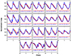 |
Fig. B.4. Same as Fig. B.3 but for the observed-model pairs considered as the silver sample. |
| In the text | |
|
Fig. B.5. Light curves of the rejected model (blue)-observed (red) pairs of the 10 BL Her stars in the LMC. Note that the BL Her star Gaia DR3 4657832869370030720 has sparse epoch photometry in the G band. |
| In the text | |
|
Fig. B.6. Same as Fig. 3 but for both the gold sample and the silver sample of the BL Her models. The open-faced histogram bars and circles represent the silver sample BL Her models. |
| In the text | |
|
Fig. B.7. Same as Fig. B.3 but for their OGLE counterparts. Missing subplots indicate lack of their OGLE counterparts and/or lack of VI photometric data. |
| In the text | |
|
Fig. B.8. Same as Fig. 6 but for the observed BL Her star with the bump feature Gaia DR3 4658440315161900928. |
| In the text | |
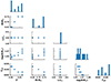 |
Fig. B.9. Same as Fig. 7 but for the observed BL Her star Gaia DR3 4658440315161900928. |
| In the text | |
Current usage metrics show cumulative count of Article Views (full-text article views including HTML views, PDF and ePub downloads, according to the available data) and Abstracts Views on Vision4Press platform.
Data correspond to usage on the plateform after 2015. The current usage metrics is available 48-96 hours after online publication and is updated daily on week days.
Initial download of the metrics may take a while.